Predicting the 305-Day Milk Yield of Holstein-Friesian Cows Depending on the Conformation Traits and Farm Using Simplified Selective Ensembles

Abstract

In animal husbandry, it is of great interest to determine and control the key factors that affect the production characteristics of animals, such as milk yield. In this study, simplified selective tree-based ensembles were used for modeling and forecasting the 305-day average milk yield of Holstein-Friesian cows, depending on 12 external traits and the farm as an environmental factor. The preprocessing of the initial independent variables included their transformation into rotated principal components. The resulting dataset was divided into learning (75%) and holdout test (25%) subsamples. Initially, three diverse base models were generated using Classifiction and Regression Trees (CART) ensembles and bagging and arcing algorithms. These models were processed using the developed simplified selective algorithm based on the index of agreement. An average reduction of 30% in the number of trees of selective ensembles was obtained. Finally, by separately stacking the predictions from the non-selective and selective base models, two linear hybrid models were built. The hybrid model of the selective ensembles showed a 13.6% reduction in the test set prediction error compared to the hybrid model of the non-selective ensembles. The identified key factors determining milk yield include the farm, udder width, chest width, and stature of the animals. The proposed approach can be applied to improve the management of dairy farms.

1. Introduction

Numerous studies have found associative connections between external characteristics of dairy cows and their milk production [1,2,3]. The 305-day milk yield is dependent on many other factors, such as the genetic potential of the animals, fertility, health status, environmental comforts, etc. Therefore, establishing which connections between the various factors determine a given productive trait and predicting its values, including milk yield, is an important research issue for improving economic profitability and dairy farm management.

In dairy science, many studies are based on modeling of collected empirical data using modern computer-based statistical techniques. These techniques enable determination of not only linear-type dependencies using standard statistical approaches, such as multiple linear regression (MLR), but also complex and hidden local dependencies between examined variables with significantly better predictive ability. A review paper [4] showed that the health and productivity of milk cows depend on various parameters and that numerous researchers have recognized the potential of machine learning (ML) as a powerful tool in this field. In [5], MLR, random forest (RF), and artificial neural networks (ANN) were used to determine dairy herd improvement metrics, with the highest impact on the first-test-day milk yield of primiparous dairy Holstein cows. MLR and ANN were used in [6] for 305-day milk yield prediction. In [7], the decision tree (DT) method was used to study lactation milk yield for Brown Swiss cattle, depending on productivity and environmental factors. The live body weight of Pakistani goats was predicted in [8] depending on morphological measurements using classification and regression trees (CART), Chi-square Automatic Interaction Detector (CHAID), and multivariate adaptive regression splines (MARS). In [9], DT was used to assess the relationship between the 305-day milk yield and several environmental factors for Brown Swiss dairy cattle. Fenlon et al. [10] applied logistic regression, generalized additive models, and ensemble learning in the form of bagging to model milk yield depending on age, stage of suckling, calving, and energy balance measures related to the animals. Four ML methods were tested by Van der Heide et al. [11]: majority voting rule, multiple logistic regression, RF, and Naive Bayes for predicting cow survival as a complex characteristic, which combines variables such as milk production, fertility, health, and environmental factors. The authors of [12] studied cattle weight using active contour models and bagged regression trees.

Other publications in the field of study related to dairy cows and the use of data mining and ML methods are [13,14,15,16]. In a broader aspect, predictive ML models and algorithms are essential to make intelligent decisions for efficient and sustainable dairy production management using information, web information, and expert systems [17]. As stated in [17], modern dairy animals are selected for physical traits that directly or indirectly contribute to high milk production. In particular, this motivates the development of models and tools for assessing and forecasting expected milk based on a limited number of easily measurable factors, such as the main external characteristics of the animals.

A new approach based on ensemble methods using bagging, boosting, and linear stacking of their predictions was developed in this paper to increase the predictive ability of the models. The essential part of modeling is the construction of selective ensembles, which reduce the number of trees in the ensemble and, at the same time, improve the performance of the model. Many researchers are actively studying this problem. The complete solution to the problem of choosing a subset of trees in the ensemble to minimize generalization errors comes down to $2^{tn}-1$ possibilities, where $tn$ is the number of trees. Such an algorithm is NP-complete [18]. For this reason, various heuristic algorithms for pruning and building selective ensembles are being developed. Some of the well-known results on selective ensembles of decision trees and ANN are based on genetic algorithms [19,20]. In [19], the resulting ensemble model is a weighted combination of component neural networks, the weights of which are determined by the developed algorithm so as to reduce the ensemble size and improve the performance. The algorithm selects the trees with weights greater than a preset threshold to form an ensemble with a reduced number of trees. This algorithm was further modified and applied to build decision tree selective ensembles in [20]. A significant reduction in the number of trees was achieved, from 20 to an average of 8 trees for 15 different empirical datasets. It is also believed that to obtain more efficient models, the components of an ensemble must be sufficiently different [21,22,23]. Applied results in this area can be found in [24,25,26] and others.

This paper contributes to statistical data modeling and machine learning by developing a framework based on a new heuristic algorithm for constructing selective decision tree ensembles. The ensembles are built with rotation CART ensembles and bagging (EBag), as well as rotation-adaptive resampling and combining (Arcing) algorithms. The simplified selective ensembles are built from the obtained models based on the index of agreement. This approach not only reduces the number of trees in the ensemble but also increases the index of agreement and the coefficient of determination and reduces the root mean square error (RMSE) of the models. In addition, combinations by linear stacking of models were obtained that satisfy four diversity criteria. The proposed approach was applied to predict the 305-day milk yield of Holstein-Friesian cows depending on the conformation traits of the animals and their breeding farm. Comparative data analysis with the used real-world datasets showed that constructed selective ensembles have higher performance than models with non-selective ensembles.

2. Materials and Methods

All measurements of the animals were performed in accordance with the official laws and regulations of the Republic of Bulgaria: Regulation No. 16 of 3 February 2006 on protection and humane treatment in the production and use of farm animals, the Regulation amending of the Regulation No. 16 (last updated 2017), and the Veterinary Law (Chapter 7: Protection and Human Treatment of Animals, Articles 149–169). The measurement procedures were carried out in compliance with Council Directive 98/58/EC concerning the protection of animals kept for farming purposes. All measurements and data collection were performed by qualified specialists from the Department of Animal Husbandry—Ruminants and Dairy Farming, Faculty of Agriculture, Trakia University, Stara Zagora, Bulgaria, with methodologies approved by the International Committee for Animal Recording (ICAR) [27]. The data do not apply to physical interventions, treatments, experiments with drugs, or other activities harmful or dangerous to animals.

2.1. Description of the Analyzed Data

In this study, we used measurements from n = 158 Holstein-Friesian cows from 4 different farms located within Bulgaria. One productive characteristic was recorded: 305-day milk yield.

Table 1. Description of the variables used in statistical analyses.

Variable	Description	Type	Measure
Milk305	305-day milk yield	Scale	kg
Stature	Stature	Ordinal	1, 2, …, 9; Short—Tall
ChestW	Chest width	Ordinal	1, 2, …, 9; Narrow—Wide
RumpW	Rump width	Ordinal	1, 2, …, 9; Narrow—Wide
RLRV	Rear legs (rear view)	Ordinal	1, 2, …, 9; Hock in-Parallel
RLSV	Rear leg set (side view)	Ordinal	1, 2, …, 5 (Transformed); Strait/Sickled—Ideal
HockD	Hock development	Ordinal	1, 2, …, 9; Filled—Dry
Bone	Bone structure	Ordinal	1, 2, …, 9; Coarse—Fine and thin
FootA	Foot angle	Ordinal	1, 2, …, 5 (Transformed); Low/Steep—Ideal
FootD	Foot depth	Ordinal	1, 2, …, 9; Short—Tall
UdderW	Udder width	Ordinal	1, 2, …, 9; Narrow—Wide
Locom	Locomotion	Ordinal	1, 2, …, 9; Severe abduction— No abduction
Lameness	Lameness	Ordinal	1, 2, 3; Walks unevenly—Very lame
Farm	Farm number	Nominal	1, 2, 3, 4

provides a description of the initial variables used. The collection of data and the choice of variables were based on the following considerations. It is well known from practice and research that the form and level of development of conformation traits depend on heritability and phenotypic characteristics of animals and influence their productivity, health, and longevity. The linear traits used were measured and evaluated for the animals according to the recommendations of the International Agreement on Recording Practices for conformation traits of ICAR (pp. 199–214, [27]). Our dataset of approved standard traits includes stature, chest width, rump width, rear leg set, rear legs (rear view), foot angle, and locomotion. Hock development and bone structure are representatives of the group of common standard traits. In addition, three other traits eligible under ICAR rules were recorded: foot depth, udder width, and lameness. For the present study, from each group, we selected those traits that have the highest coefficient of heritability and correlation with the 305-day milk yield, established as per Bulgarian conditions in [28,29]. The dataset includes the variable Farm to account for growing conditions, the environment, the influence of the herd, and other implicit and difficult-to-measure factors.

External traits are described individually as ordinal variables. This scale complies with the standards of the ICAR [27]. The examined traits have two types of coding. The two traits (variables RLSV and FootA) are transformed, resulting in two opposite disadvantages in the ranking scale from 1 to 5 with ascending positive evaluation of the trait, in accordance with the evaluation instructions as per the type of ICAR. All other traits were measured linearly from one biological extreme to the other. The range of scores is from 1 to 9, and improvement of the characteristic corresponds to a higher value. The variable Farm is of categorical type, with 4 different values. The distribution by number of cows in the farms is 54, 32, 34, and 38.

It should be noted that in the general case, the relationships between the variables for exterior traits the productive and phenotypic characteristics of Holstein cattle are considered to be nonlinear (for example, [30]). Therefore, the machine learning approach has a better perspective to reveal the deep multidimensional dependencies between them.

Table 1 and

Table 2. Nomenclature of the notations ¹.

Notation	Description	Type
ARC	Arcing	method
CART	Classification and regression trees	method
CV	Cross-validation	out-of-sample testing
EBag	CART ensembles and bagging	method
PCA	Principal component analysis	method
IA, d	Index of agreement [31]	statistic
WSRT	Wilcoxon signed rank test	statistical test
RT	Reduced tree	list of trees
AR9, AR10	Arcing model (predicted values)	variable
EB, EB15, EB40	EBag model (predicted values)	variable
Hybr1, Hybr2	Stacked linear model (predicted values)	variable
PC1, PC2, …	Principal component, factor variable	variable
SSAR9	Simplified selective ARC model (predicted values)	variable
SSEB, SSEB11, SSEB25	Simplified selective EBag model (predicted values)	variable

¹ All variable names are in italic style.

list notations used in this paper.

2.2. Modeling Methods

Statistical analyses of the data were performed using principal component analysis (PCA), factor analysis, and ensemble methods EBag and ARC. We used EBag and ARC as ensemble methods based on bagging and boosting, respectively. The main types of ensemble methods, their characteristics, advantages, and disadvantages are discussed in [21,23,32].

2.2.1. Principal Component Analysis and Exploratory Factor Analysis

PCA is a statistical method for transforming a set of correlated variables into so-called principal components (PCs) [33]. The number of variables is equal to the number of extracted PCs. When the data include several strongly correlated variables, their linear combination can be replaced by a new common artificial variable through factor analysis. In this case, the number of initial variables is reduced at the cost of certain losses in the total variance explained by the new sample. Following the rotation procedure, the resulting rotated factor variables are non-correlated or correlate weakly with one another. These can be used in subsequent statistical analyses. PCA was used in [34,35].

2.2.2. CART Ensemble and Bagging (EBag)

An ensemble is a model that includes many single models (called components) of the same type. In our case, the components are decision trees constructed using the powerful ML and data-mining CART method [36]. CART is used for regression and classification of numerical, ordinal, and nominal datasets. For example, let an initial sample of $n$ observations $\{\mathrm{Y},\mathrm{X}\}$ be given, where $\mathrm{Y}=\left\{y_{1,}{y}_{2,}\dots ,y_n\right\}$ is the target variable and $\mathrm{X}=\left\{X_1,X_2,\dots ,X_p\right\},p\ge 1$ are independent variables. The single CART model is a binary tree structure, $T$, obtained by recursively dividing the initial dataset into disjoint subsets called nodes of the tree. The predicted value for each case in the node, ${\tau }_{\ell }\in T$, is the mean value of $\mathrm{Y}$ of cases in ${\tau }_{\ell }$. The root of the tree contains all the initial observations, and its prediction is the mean value of the sample.

For each splitting of a given node, ${\tau }_{\ell }$, the algorithm of the method selects a predictor, $X_k$, and its threshold case, $X_{k,\theta }$, from all or from a pool of variables, $\mathrm{X}$, and cases in ${\tau }_{\ell },$ to minimize some preselected type of model prediction error. The division of cases from ${\tau }_{\ell }$ is performed according to the rule: if $X_{k,i}\le X_{k,\theta }$, $\mathrm{X}\in {\tau }_{\ell }$ then the observation with index $i$ is assigned to the left child node of ${\tau }_{\ell }$—and in the case of $X_{k,i}>X_{k,\theta }$, to the right child node of ${\tau }_{\ell }$. The growth of the tree is limited and stopped by preset hyperparameters (depth of the tree, accuracy, etc.). Thus, all initial observations are classified into terminal nodes of the tree. If a training sample is specified, the CART model function can be written as [33]:

$$\widehat{\mu }\left(\mathrm{X}\right)=\sum _{\tau \in T}\widehat{Y}\left(\tau \right)I_{[\mathrm{X}\in \tau ]}=\sum _m^{\ell =1}\widehat{Y}\left({\tau }_{\ell }\right)I_{\left[\mathrm{X}\in {\tau }_{\ell }\right]}$$

(1)

where:

$$\widehat{Y}\left({\tau }_{\ell }\right)=\overline{Y}\left({\tau }_{\ell }\right)=\frac{1}{n\left({\tau }_{\ell }\right)}{\displaystyle \sum _{{\mathrm{X}}_i\in {\tau }_{\ell }}^{}{y}_i},I_{\left[\mathrm{X}\in {\tau }_{\ell }\right]}=\{\begin{array}{c}1,\mathrm{X}\in {\tau }_{\ell }\\ 0,\mathrm{X}\notin {\tau }_{\ell }\end{array}$$

(2)

where $m$ is the number of terminal nodes of the tree, and $n\left({\tau }_{\ell }\right)$ is the number of observations in node ${\tau }_{\ell }$. For each case $i$, ${\widehat{y}}_i=\widehat{\mu }\left({\mathrm{X}}_i\right)$ is the predicted value for the observation, ${\mathrm{X}}_i$.

An example of a CART model with 2 independent variables and 5 nodes is shown in Figure 1.

CART ensembles and bagging is an ensemble method with ML for classification and regression proposed by Leo Breiman in [37]. For ensembles, the training set is perturbed repeatedly to generate multiple independent CART trees, and then the predictions are averaged by simple voting. In this study, we used the software engine CART ensembles and bagger included in the Salford Predictive Modeler [38].

In order to compile the ensemble, the researcher sets the number of trees, type of cross-validation, number of subsets of predictors for the splitting of each branch of each tree, limits for the minimum number of cases per parent and child node, and some other hyperparameters. The method’s main advantage is that it leads to a dramatic decrease in test-set errors and a significant reduction in variance [39].

In terms of generating, the tree components of the ensemble are characterized by considerable differences in their performance and, individually, do not have high statistical indices. For this reason, in the literature, these are called “weak learners”. However, after averaging, the statistics are adjusted, and the final ensemble model (for classification or regression) is more efficient. Component trees, which worsen the ensemble’s statistics in any statistical measure, are called “negative” trees. Various heuristic algorithms have been developed to reduce the impact of these trees [19,26].

2.2.3. Adaptive Resampling and Combining Algorithm (Arcing)

Another approach that uses ensemble trees is based on the boosting technique first proposed in [40]. A variant of boosting is the Arcing algorithm developed and studied by Breiman in [39], also known as Arc-x4. The family of Arc-x(h) algorithms is differentiated from Adaboost [40] by the simpler weight updating rule in the form:

$$w_{t+1}(V_i)=\frac{1+m{(V_i)}^h}{{\displaystyle \sum _i\left(1+m{(V_i)}^h\right)}}.$$

(3)

where $m(V_i)$ is the number of misclassifications of instance $V_i$ by models generated in the previous iterations, and $1,2,\dots ,t$, h is an integer. In this way, the ensemble components are generated sequentially and penalize resampling in the cases that yield bad predictions up to the current step, $t$. Breiman showed that Arcing had error performance comparable to that of Adaboost.

Combining multiple models and applying any of the two methods—bagging or arcing—leads to a significant variance reduction, whereby arcing is more successful than bagging in test-set error reduction [39].

2.2.4. Proposed Simplified Selective Ensemble Algorithm

To improve predictive performance, we further developed the algorithm for building simplified selective ensembles that we recently proposed in [41] for time series analysis. In this study, used it in the case of a non-dynamic data type. We applied the algorithm separately for two types of ensembles from CART trees: with bagging and boosting. The simplified selective algorithm is presented for the case of EBag. It consists of the following steps:

• Step 1: Calculation of index of agreement (IA), $d_E$ [31], for a selected initial EBag model, $EBtn$, with $tn$ component trees;
• Step 2: Cycle with the application of a pruning criterion to live-out the j-th component tree $T_j$ for $j=1,2,\dots ,tn$… and calculation of reduced tree $R{T}_j$;
• Step 3: Calculation of IA $d_j$ for $j=1,2,\dots ,tn$ of all obtained reduced trees, $R{T}_j$. If $d_j>d_E$, then the tree, $T_j$, is considered “negative” and subject to possible removal from the ensemble. If the number of negative trees is $s$, we denote their set with $ss=\{T_1^{-},T_{{}_2}^{-},\dots ,T_s^{-}\}$, where $T_j^{-}$ is the negative tree.
• Step 4: Building $s$ simplified selective models by removing cumulative sums from negative trees using the expression:

$$SSE{B}_{tn-k}=\frac{tn.EBtn-{\displaystyle \sum _{j=1}^{k}s{s}_j}}{tn-k},k=1,2,\dots ,s.$$

(4)

In this way, removing the “negative” trees improves the IA of the initial EBag model and generates many new ensemble models for $k=1,2,\dots ,s$. The maximum simplified selective tree is obtained at $k=s$.

To implement the simplified selective algorithm, we used the generated EBag and ARC component trees using the ensembles and bagger engine of SPM software [38] and the authors’ code in Wolfram Mathematica [42]. A detailed description of the simplified selective algorithm is given in Algorithm 1.

Algorithm 1: Simplified selective ensemble

Input: dataset E, Tj, tn // E is an ensemble model of weak learners Tj, j = 1,2, …,tn. E is        an averaged sum of Tj.   Output: SSE, sn // SSE is a vector of indices of the resulting simplified selective ensembles, sn        is the number of simplified selective models in SSE.      k ← 0; // k is the number of the negative trees (learners).      sind ← Ø; // sind is a list or array with the indices of negative trees or learners.      dE ← IA(E); // Value of the Index of agreement (IA) of E ([31], see also Equation (5).      j ← 1;      While j <= tn do            end;      s ← k;      sn ← tn-s;      If [ s = 0 then        Break [Algorithm 1];      ]; // in this case, there are not any simplified selective models.      j ← 1;      SSE ← Ø;      While [ j <= (tn-s) do

2.2.5. Methodology

In this study, regression models were constructed to determine the influence of the observed external characteristics of Holstein-Friesian cows and the farm on milk quantity and to predict the values of 305-day milk yield. First, EBag and arcing ensembles and corresponding simplified selective models were built, and their predictions were then combined linearly in stacked models according to the stacked generalization paradigm developed by Wolpert [43].

Our study was carried out under the following framework (see also Figure 2):

• Transformation of 12 independent variables for the external traits using the PCA method and factor analysis and obtaining 11 PCs (factor variables), denoted as PC1, PC2, …, PC11;
• Random splitting of the sample for Milk305 into learning and test datasets at a ratio of 75%:25%; the learning sample is denoted by the variable Milk_miss40, where 25% (40 cases) of the values for milk yield are considered as missing;
• Building and examination of rotation EBag, simplified selective EBag, and rotation ARC regression models with predictors PC1, …, PC11, and Farm to predict Milk_miss40;
• Verification of the condition for diversity and selection of three base models using Wilcoxon signed-rank test (WSRT);
• Determination of the relative importance of predictors in the base models;
• Assessment of models against the initial full-sample Milk305.
• Combination of the selected base models using weights and assessment of the resulting stacked model.
• Assessment of model performance for the 25% holdout test sample.

Figure 2. Framework of the study.

Figure 2. Framework of the study.

For application of the stacking paradigm in particular, the number of base models at the first stage has to be between 3 and 8. In addition, these models need to be differentiated from each other according to some diversity criteria [21,22,23].

2.2.6. Evaluation Measures

The quality of the built models was assessed and compared using standard measures of prediction accuracy: root mean squared error (RMSE), mean absolute percentage error (MAPE), goodness-of-fit measure (coefficient of determination $R^2$), and index of agreement (IA) $d$ [31], defined as follows:

$$\begin{array}{l}\mathrm{RMSE}=\sqrt{\frac{1}{n}{\displaystyle \sum _{k=1}^n{\left(P_k-Y_k\right)}^2}},\mathrm{MAPE}=\frac{100}{n}{\displaystyle \sum _{k=1}^n\left|\frac{P_k-Y_k}{Y_k}\right|},\\ R^2=\frac{{\left\{{\displaystyle \sum _{k=1}^n\left(P_k-\overline{P}\right)\left(Y_k-\overline{Y}\right)}\right\}}^2}{{\displaystyle \sum _{k=1}^n{\left(P_k-\overline{P}\right)}^2.}{\displaystyle \sum _{k=1}^n{\left(Y_k-\overline{Y}\right)}^2}},\mathrm{IA}=d=1-\frac{{\displaystyle \sum _{k=1}^n{\left(P_k-Y_k\right)}^2}}{{\displaystyle \sum _{k=1}^n{\left(\left|P_k-\overline{Y}\right|+\left|Y_k-\overline{Y}\right|\right)}^2}},\end{array}$$

(5)

where $Y_k$ and $\overline{Y}$ are the values and the mean of the dependent variable, $Y$, respectively; $P_k$ and $\overline{P}$ are the predicted values and their mean, respectively; and $n$ is the sample volume. Among these measures, a good predictive model should have a value close to 0 for RMSE and MAPE and a value close to 1 for $R^2$ and IA. IA is not a measure of correlation or association in the formal sense but a measure of the degree to which a model’s predictions are error-free [31].

Furthermore, the nonparametric WSRT is used to compare diversity between the predictive models [44]. This test does not assume that the data follow the normal distribution.

3. Results and Discussion

3.1. Data Preprocessing

Table 3. Descriptive statistics of the measured data ¹.

Variable	Mean	5% Lower Bound of Mean	5% Upper Bound of Mean	Median	Std. Dev.	Skewness	Kurtosis
Milk305, kg	6812.16	6451.67	7172.66	6784.25	2294.12	0.282	−0.866
Milk_miss40, kg	6789.32	6359.29	7226.36	6041.00	2397.14	0.310	−0.896
Milk_40, kg	6879.54	6244.59	7514.49	6743.19	1985.37	0.182	−0.960
Stature	4.68	4.39	4.96	5.00	1.83	−0.228	−0.558
ChestW	6.51	6.25	6.77	7.00	1.65	−0.358	−0.569
RumpW	6.09	5.91	6.28	6.00	1.18	0.241	−0.687
RLRV	4.91	4.68	5.14	5.00	1.45	0.054	0.291
RLSV	3.95	3.79	4.11	4.00	1.01	−0.577	−0.631
HockD	5.29	5.06	5.52	5.00	1.48	0.038	−0.170
Bone	6.13	5.89	6.37	6.00	1.53	−0.260	−0.477
FootA	4.51	4.42	4.61	5.00	0.59	−0.786	−0.349
FootD	6.42	6.24	6.59	7.00	1.10	−0.310	−1.434
UdderW	5.72	5.42	6.02	6.00	1.92	−0.368	−0.484
Locom	5.32	5.11	5.53	5.00	1.34	−0.092	−0.530
Lameness	1.65	1.55	1.76	2.00	0.67	0.535	−0.713

¹ Std. Err. Skewness is 0.193; for Milk_miss40, 0.223; for Milk_40, 0.374. Std. Err. Kurtosis is 0.384; for Milk_miss40, 0.442; for Milk_40, 0.733.

shows the results of the descriptive statistics of the initial variables from Table 1. We see that the values of skewness and kurtosis for all variables are close to zero, and we can assume that the distribution of all variables is close to normal.

3.2. PCA Results

During the initial data processing, multicollinearity was found between the considered 12 independent variables for conformation traits from Table 1. In order to reduce the influence of multicollinearity and improve the accuracy of the regression models, these 12 initial variables were transformed into independent variables using exploratory factor analysis and PCA [33]. The goal is to retain information and preserve the total variance explained following this transformation as much as possible. The basic assumptions for procedural application are fulfilled, namely: close to a normal distribution of the 12 variables and small determinant of their correlation matrix, $\det =0.019\approx 0$. In addition, the adequacy verification of factor analysis indicates that the Kaiser–Meyer–Olkin (KMO) measure of sampling adequacy is 0.658 > 0.5, and the significance of the Bartlett’s test of sphericity is Sig. = 0.000.

With the help of nonparametric Spearman’s rho statistics R, the following correlation coefficients were found between the dependent variable, Milk305, and the 12 measured variables, respectively: with the variable UdderW, R = 0.685; with Stature, R = 0.501; with ChestW, R = 0.492; and with Bone R = 0.343. Other significantly correlated Spearman’s rho coefficients are: R(Stature, UdderW) = 0.558, R(Stature, RumpW) = 0.508, R(Stature, ChestW) = 0.466, R(Bone, Stature) = 0.466, and R(Laminess, Locom) = −0.929. All correlation coefficients are significant at the 0.01 level (2-tailed). Research into this type of linear correlation is a known approach, including external traits [28,29]. This often leads to establishing both positive and negative linear correlations (e.g., R(Laminess, Locom) = −0.929), etc.). The latter can lead to an inaccurate interpretation of the influence of some external traits, the interactions of which are primarily nonlinear and difficult to determine [30].

The next step is to conduct factor analysis. In our case, 12 PCs were preset for extraction using the PCA method. Due to the strong negative correlation R(Laminess, Locom) = −0.908, these two variables were grouped in a common factor. This resulted in 11 factors extracted from the 12 independent variables. The factors were rotated using the Promax method. The resulting rotated matrix of factor loadings is shown in

Table 4. Rotated pattern matrix with 11 PCs generated using Promax ¹.

Initial Variable	Principal Components (Factor Variables)
	PC1	PC2	PC3	PC4	PC5	PC6	PC7	PC8	PC9	PC10	PC11
Locom	0.978	−0.009	−0.001	0.007	0.000	0.016	0.028	0.011	0.025	0.002	−0.032
Lameness	−0.976	−0.009	−0.001	0.007	0.000	0.016	0.028	0.011	0.025	0.002	−0.032
RumpW	0.000	0.998	0.000	0.000	0.000	0.001	0.000	0.000	0.000	0.001	0.002
ChestW	0.000	0.000	0.998	0.001	0.000	0.000	0.000	0.000	0.000	0.001	0.001
UdderW	0.000	0.000	0.001	0.995	0.000	0.000	0.000	0.000	0.000	0.002	0.006
RLRV	0.000	0.000	0.000	0.000	1.000	0.000	0.000	0.000	0.000	0.000	0.000
FootD	0.000	.001	0.000	0.000	0.000	0.999	−0.001	0.000	−0.001	0.001	0.001
RLSV	0.000	0.000	0.000	0.000	0.000	−0.001	1.000	−0.001	−0.001	0.000	0.002
FootA	0.000	0.000	0.000	0.000	0.000	0.000	−0.001	1.000	−0.001	0.000	0.001
HockD	0.000	0.000	0.000	0.000	0.000	−0.001	−0.001	−0.001	1.000	0.000	0.002
Bone	0.000	0.002	0.002	0.002	0.001	0.001	0.000	0.000	0.000	0.995	0.003
Stature	0.000	0.006	0.003	0.011	0.000	0.001	0.002	0.001	0.002	0.004	0.986

¹ Extraction method: principal component analysis; Rotation method: Promax with Kaiser normalization; rotation converged in six iterations.

. The extracted 11 factor-score variables are very well differentiated. We denote them by PC1, PC2, …, PC11. These 11 variables account for 99.278% of the total variance of the independent continuous variables. The residual variance is 0.722 and can be ignored. The correspondence between the initial 12 linear traits and the resulting 11 PCs is given in Table 4. The coefficients of the factor loadings are sorted by size, and coefficients with an absolute value below 0.1 are suppressed [33].

Considering that the coefficients along the main diagonal in the rotated pattern matrix of Table 4 are equal to 1 or almost 1, in subsequent analyses, we can interpret each generated factor as a direct match with the corresponding initial variable, except PC1, which groups Locom and Lameness.

3.3. Building and Evaluation of Base Models

To model and predict the milk yield dataset, Milk_miss40, we used the eleven PCs and Farm variables as predictors. The aim is to build between 3 and 8 base models that meet the diversity requirement, as recommended in the stacking paradigm [22,43,45]. In this study, we set the following four diversity criteria:

(C1)

different learning datasets for each tree and ensemble derived from the algorithms;

(C2)

different methods and hyperparameters to build the ensembles;

(C3)

different number of trees in the ensemble models;

(C4)

different types of testing or validation.

3.3.1. CART Ensembles and Bagging and Simplified Selective Bagged Ensembles

First, numerous CART-EBag models with different numbers of component trees $(tn=10,15,20,\dots ,60)$ were built. The hyperparameters were changed as follows: minimum cases in parent node to minimum cases in child node-14:7, 10:5, 8:4, 7:4. Cross-validation was varied from CV-5 fold, 10 fold, and 20-fold. Of these models, two ensemble models, EB15 and EB40, were selected, with $tn=15$ and $tn=40$ trees. The subsequent increase in the number of trees in the ensemble and the tuning of the hyperparameters led to a decrease in the statistical indices of the ensembles. These two models were used to generate selective ensembles according to the algorithm described in Section 2.2.4. Four negative trees were reduced from model EB15. The resulting simplified selective ensemble with 11 component trees is denoted as SSEB11. Accordingly, for the second model, EB40, 15 negative trees were identified, and after their removal, model SSEB25 with 25 component trees was obtained.

The analysis of the statistical indices of simplified selective ensembles revealed some special dependencies. We will demonstrate the main ones for the components of the EB40 model. Figure 3a illustrates the values of $d_j,j=1,2,\dots ,40$, calculated for all component trees compared against the $d_E$ of the initial ensemble. Values greater than $d_E$ correspond to negative trees. Figure 3b–d show the change in the statistical indices for the generated selective models, $SSE{B}_{40-k},k=1,2,\dots ,15$, obtained from EB40 after the removal of the cumulative sums of negative trees in (4).

Figure 3b shows that the curves IA and $R^2$ of ensembles $SSE{B}_{40-k},k=1,2,\dots ,s$ increase monotonically with the removal of each subsequent negative tree, $T_j^{-}$, as the values of $R^2$ increase faster. The behavior of the RMSE is inversely proportional and decreases monotonically with increased $k$. We found that with the removal of each subsequent negative tree, all statistics (5) improve, excluding MAPE. In our case, for the selected SSEB25 model and Milk305, IA increases by 0.5%, $R^2$ increases by 1.7%, RMSE is reduced by 12.8%, and MAPE is reduced by 6.6% compared to the initial ensemble, EB40 (see Section 3.3.4.

3.3.2. Arcing and Simplified Selective Arcing Models

Numerous ARC models with different hyperparameters were built by varying the number of component trees:$tn=5,10,\dots ,30$. The hyperparameters were changed as follows: minimum cases in parent node to minimum cases in child node-14:7, 10:5, 8:4, 7:4, 6:3. Cross-validation was varied: CV-5-fold, 10-fold, and 20-fold. One model with 10 components was selected from the obtained ARC models, denoted as AR10, which satisfies the diversity criteria C1, …, C4 with EB15 and EB40. This model was used to generate a selective ensemble with nine component trees denoted by SSAR9.

3.3.3. Diversity of the Selected Base Models and Their Hyperparameters

The diversity criteria between the base models were checked using a two-related-samples WSRT. The resulting statistics are given in

Table 5. Test statistics for diversity verification among the selected base models ^a.

Statistics	Models
	EB15-EB40	EB15-AR10	AR10-EB40	SSEB11-SSEB25	SSEB11- SSAR9	SSEB25- SSAR9
Z	−3.440 b	−3.475 b	−2.006 b	−2.360 b	−3.480 b	−2.332 b
Asymp. Sig. (2-tailed)	0.001	0.001	0.045	0.018	0.001	0.020

^a Wilcoxon signed ranks test. ^b Based on negative ranks.

. Because they are all significant at a level of $\alpha =0.05$, we can assume that the selected base models are different [44].

Table 6 shows the relevant hyperparameters of the base models in the following two groups:

• Group A: EB15, EB40, and AR10;
• Group B: SSEB11, SSEB25, and SSAR9.

Table 6. Hyperparameters of the selected base models.

Hyperparameter	Model
	EB15, SSEB11	EB40, SSEB25	AR10, SSAR9
Number of trees in ensemble	15, 11	40, 25	10, 9
Minimum cases in parent node	8	8	10
Minimum cases in child node	4	4	1
Independent variables	Farm, PC1, PC2, …, PC11	Farm, PC1, PC2, PC4, PC5, PC7, …, PC11	Farm, PC1, …, PC6, PC9, PC10, PC11
Type of the k-fold cross-validation	10-fold	10-fold	20-fold

Table 6. Hyperparameters of the selected base models.

Hyperparameter	Model
	EB15, SSEB11	EB40, SSEB25	AR10, SSAR9
Number of trees in ensemble	15, 11	40, 25	10, 9
Minimum cases in parent node	8	8	10
Minimum cases in child node	4	4	1
Independent variables	Farm, PC1, PC2, …, PC11	Farm, PC1, PC2, PC4, PC5, PC7, …, PC11	Farm, PC1, …, PC6, PC9, PC10, PC11
Type of the k-fold cross-validation	10-fold	10-fold	20-fold

The number of variables for splitting each node on each tree was set to 3. It should also be noted that the indicated value, k, of the cross-validation is applied to all trees in the respective ensemble model.

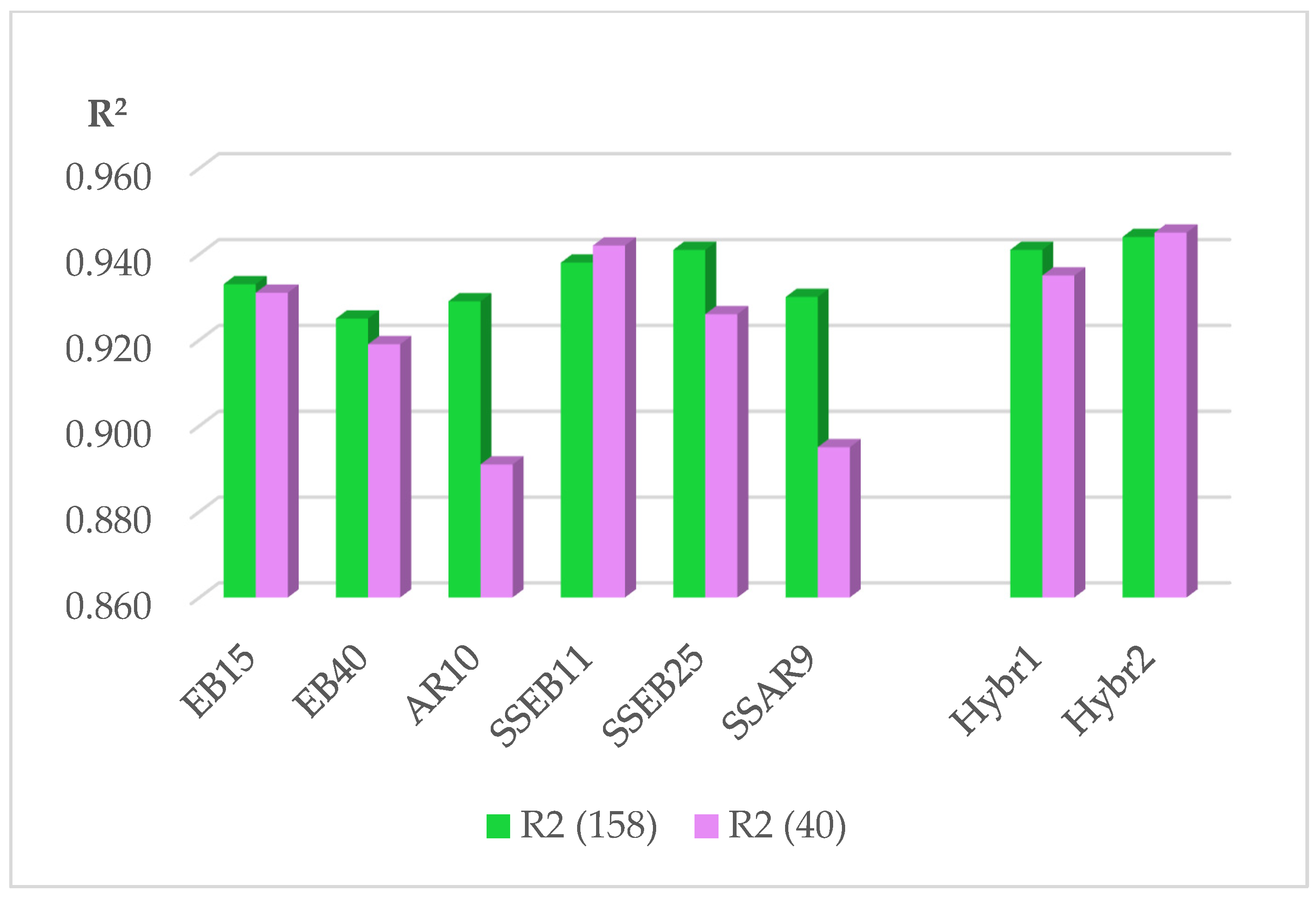
3.3.4. Evaluation Statistics of the Selected Base Models

First, let us estimate the reduction in the number of trees in the simplified selective ensembles. For the three base models, we have: from EB15 to SSEB11, 4 trees; from EB40 to SSEB25, 15 trees; and from AR10 to SSAR9, 1 tree. The relative reductions are 25%, 37.5%, and 10%, or an average of 30%.

The performance statistics (5) of the selected two groups of base models for predicting the reduced dependent variable Milk_miss40 were evaluated and compared. In addition, the predicted values of these models were also compared against the initial sample, Milk305 with 158 cases; Milk_miss40 with 118 cases; and the holdout test sample, and Milk_40 with 40 cases, not used in the modeling procedure. The obtained basic statistics of predictive models are shown in the first six columns of

Table 7. Summary statistics of the predictions of obtained models against the measured values of the dependent variables.

Measure	Base Model Group A			Base Model Group B			Linear Combinations
	EB15	EB40	AR10	SSEB11	SSEB25	SSAR9	Hybr1	Hybr2
Mean, 158	6739.11	6797.17	6872.41	6747.79	6790.98	6871.63	6787.81	6778.75
Mean, 118	6755.05	6810.56	6836.70	6758.16	6811.57	6844.17	6787.88	6779.66
Mean, 40	6692.06	6757.64	6977.76	6717.18	6730.25	6952.66	6787.61	6776.05
Std. Dev., 158	2086.27	2119.82	2029.76	2118.99	2143.82	2081.68	2062.66	2100.91
Std. Dev., 118	2163.54	2187.59	2077.31	2191.88	2225.50	2131.27	2132.25	2169.99
Std. Dev., 40	1864.37	1931.58	1903.79	1913.43	1907.36	1951.61	1867.60	1908.38
$R^2,158$	0.933	0.925	0.929	0.938	0.941	0.930	0.941	0.944
$R^2,118$	0.934	0.928	0.941	0.939	0.947	0.940	0.943	0.945
$R^2,40$	0.931	0.919	0.891	0.942	0.926	0.895	0.935	0.945
RMSE, 158	611.791	632.277	632.855	580.404	560.473	620.607	579.461	556.051
RMSE, 118	631.401	651.280	632.878	605.778	562.188	612.666	601.317	581.328
RMSE, 40	549.885	572.555	656.169	498.077	555.382	643.463	509.555	473.690
MAPE, 158 (%)	6.63	6.94	8.36	6.40	6.51	7.68	6.45	6.23
MAPE, 118 (%)	6.87	7.03	8.59	6.65	6.42	7.66	6.75	6.51
MAPE, 40 (%)	5.93	6.68	7.68	5.65	6.76	7.33	5.55	5.44
d, 158	0.9801	9.9790	0.9777	0.9824	0.9837	0.9795	0.9820	0.9837
d, 118	0.9804	0.9794	0.9796	0.9822	0.9849	0.9813	0.9820	0.9835
d, 40	0.9788	0.9777	0.9703	0.9831	0.9788	0.9722	0.9818	0.9847

. It can be seen that the performance results are similar, whereas all statistics from (5) of the selective ensembles are superior.

$R^2,158$$R^2,118$$R^2,40$ In particular, the SSEB11 model demonstrates better performance than the EB15 model from which it is derived. For example, for the whole sample, the reduction in RMSE of SSEB11 compared to EB15 is 5.1%, whereas for the test sample, Milk_40, the error is reduced by 9.26%. Similarly, model SSEB25 outperforms the source model, EB40. In this case, the improvement in RMSE for the whole sample is 11.4%, and for the holdout sample, the error is reduced by 3.0% compared to that of EB40. For SSAR9, these indices are 2% and 1.9%, respectively. Overall, the indicators of model AR10 and its simplified selective model, SSAR9, are comparatively the weakest. This can be explained by the fact that they contain the smallest number of trees, and only one negative tree has been removed from the AR10 ensemble.

3.3.5. Relative Importance of the Factors Determining Milk305 Quantity

The regression models we built were used to predict 305-day milk yield, allowing us to determine, with high accuracy, how the considered factors explain the predicted values according to their weight in the models. For better interpretation, the initial names of the variables were recorded, along with the predictors, according to Table 4. The predictor with the most significant importance in the model has the highest weight (100 scores), and the other scores are relative to it.

The results in

Table 8. Relative averaged variable importance in base models.

Predictor Variable	Model
	EB15	SSEB11	EB40	SSEB25	AR10	SSAR9
Farm	100.0	100.0	100.0	100.0	98.1	100.0
PC4 (UdderW)	67.6	67.7	64.5	66.3	64.2	60.2
PC3 (ChestW)	44.8	46.0	-	-	57.7	57.6
PC11 (Stature)	34.7	35.5	30.6	30.8	22.1	18.7
PC10 (Bone)	22.8	22.6	23.4	26.4	19.0	20.2
PC1 (Locom & Lameness)	13.5	14.5	17.1	19.8	28.5	30.0
PC9 (HockD)	6.6	6.7	12.4	14.4	36.2	38.0
PC5 (RLRV)	12.8	12.1	15.5	15.7	19.5	16.6
PC6 (FootD)	10.7	11.5	-	-	26.3	25.1
PC2 (RumpW)	9.7	10.3	11.0	11.9	30.4	30.8
PC8 (FootA)	7.8	8.0	12.3	14.0	-	-
PC7 (RLSV)	6.6	8.2	10.5	11.1	-	-

show the relative variable importance of the predictors within the built base ensemble models. As expected, the main defining variable for 305-day milk yield with the greatest importance of 100 is Farm. The other significant conformation traits, in descending order, are PC4 (UdderW), with relative weight between 60 and 68; PC3 (ChestW), 45 to 58; PC11 (Stature), 19 to 36; PC10 (Bone), 19 to 27. The conformation trails with the weakest influence are PC8 (FootA), with a relative weight of 8 to 14, and PC7 (RLSV), with a relative weight of 7 to 11. Because all predictors have an average weight of more than five relative scores, we consider them all as essential traits on which milk depends.

In an actual situation, the average values of the main conformation traits should be maintained within the limits of their lower and upper bounds of the means (5% confidence intervals). In our case, these limits are given in Table 3.

3.4. Building and Evaluation of the Linear Hybrid Models

The next stage of the proposed framework is combining the obtained predictions from the single base models. To illustrate the higher efficiency when using simplified selective ensembles, we compared the results obtained from the two groups of base models.

3.4.1. Results for Hybrid Models

Using the well-known approach of linear combinations of ensembles (see [45]), we sought to find a linear hybrid model, $\widehat{y}$, of the type

$$\widehat{y}={\alpha }_1{E}_1+{\alpha }_2{E}_2+{\alpha }_3{E}_3.$$

(6)

where $E_i,i=1,2,3$ are ensemble models that satisfy the conditions for diversity, C1, …, C4 (see Section 3.3), and the coefficients ${\alpha }_i$ are sought such that

$${\displaystyle \sum _{i=1}^3{\alpha }_i}=1,{\alpha }_i\in [0,1].$$

(7)

When varying by step $h=0.05$ in the interval $[0,1]$ and all possible combinations for ${\alpha }_i,i=1,2,3$, the following two hybrid models with the least RMSE were obtained for the test sample Milk_40:

$$Hyb{r}_1=0.55EB15+0.15EB40+0.3AR10.$$

(8)

$$Hyb{r}_2=0.75SSEB11+0.25SSAR9.$$

(9)

The main statistics of these models are given in the last two columns of Table 7. Hybrid models improve all indicators of the base models. For the holdout test sample, Milk_40, the Hybr₁ model has an RMSE equal to 509.555 kg, which is less than the errors of Group A models by 7.9% for EB15, 12.4% for EB40, and 28.8% for AR10. Accordingly, model Hybr₂ improves the statistics of Group B models. In the case of the test sample, its RMSE = 473.690 kg, which is smaller than the SSEB11, SSEB25, and SSAR9 models by 5.1%, 17.2%, and 35.8%, respectively. Furthermore, we obtained the desired result for the superiority of simplified selective models and Hybr₂ over the initial non-selective models and Hybr₁. In particular, the RMSE of Hybr₂ is smaller than that of Hybr₁ by 7% for the holdout test sample, Milk_40. MAPE coefficients of 5.5% were achieved.

A comparison of the values predicted by models (8) and (9) and the initial values for Milk305 are illustrated in Figure 4.

3.4.2. Comparison of Statistics of All Models

A comparison of the performance statistics of all eight models constructed in this study for Milk305 and Milk_40 is illustrated in Figure 5 and Figure 6. Figure 5 shows that the coefficients of determination for model AR10 and its simplified selective ensemble, SSAR9, are weaker than those of the other base models. However, despite their second largest coefficients in (8) and (9), respectively, the $R^2$ of the hybrid models is satisfactory for the small data samples studied. In the same context, Figure 6 illustrates the behavior of RMSE values, which do not deteriorate significantly in hybrid models due to their higher values in the AR10 and SSAR9 models.

Finally, we compared the RMSE and generalization error (mean squared error (MSE) = RMSE²) of the built models for a randomly selected holdout test sample, Milk_40. The results are shown in

Table 9. Holdout test-set prediction errors.

Error, Improvement	Base Model Group A			Base Model Group B			Linear Combinations
	EB15	EB40	AR10	SSEB11	SSEB25	SSAR9	Hybr1	Hybr2
RMSE, 40	549.885	572.555	656.169	498.077	555.382	643.463	509.555	473.690
Improvement by Hybr2	7.3%	11.0%	22.3%	4.9%	14.7%	26.4%	7.0%	-
MSE, 40	302,373.5	327,819.2	430,557.8	248,080.7	308,449.2	414,044.6	259,646.3	224,382.22
Improvement by Hybr2	14.1%	20.8%	39.7%	9.6%	27.3%	45.8%	13.6%	-

. The Hybr₂ model produces RMSE 7% less than that produced by Hybr₁; compared to base models, the improvement varies from 5% to 26%. The comparison by generalization error shows 13.6% and 9.6% lower values for Hybr₂ than those for Hybr₁ and model SSEB11, respectively.

4. Discussion

We investigated the relationship between the 305-day milk yield of Holstein-Friesian cows and 12 external traits and the farm in a sample of 158 cows. To evaluate the constructed models, a random holdout test subsample was used, including 25% (40 entries) from the variable Milk305 for 305-day milk yield. In order to reveal the dependence and to predict milk yield, a new framework was developed based on ensemble methods using bagging and boosting algorithms and enhanced by a new proposed simplified selective ensemble approach.

We simultaneously applied the CART ensembles and bagging and Arcing methods for livestock data for the first time. To improve the predictive ability of the models, the initial ordinal variables were transformed using factor analysis to obtain rotation feature samples. Three initial base models (group A) were selected, satisfying four diversity criteria. Numerous simplified selective ensembles were built from each of these models. Using these, a second trio of base models (group B) was selected. Predictions for each group of base models were stacked into two linear hybrid models. The models successfully predict up to 94.5% of the data for the initial and holdout test samples. The obtained results for predicting 25% holdout values of daily milk showed that the two hybrid models have better predictive capabilities than the single base models. In particular, the RMSE of hybrid model Hybr₂ from the simplified selective ensembles is 7.0% lower than that of the other hybrid model based on non-selective ensembles. The number of trees in the three selective ensembles was decreased by 27%, 37.5%, and 10%, or an average of 30%.

Our proposed approach to build selective tree ensembles is characterized by a simple algorithm, reduces the dimensionality of the ensemble, improves basic statistical measures, and provides many new ensembles to be used to satisfy the diversity criteria. In addition, in the two-level stacking procedure, we used two different criteria: increasing the index of the agreement to build simplified selective ensembles and minimizing the RMSE for choosing the stacked model.

However, some shortcomings can be noted, including the selection of base models that meet the condition of diversity, which remains a challenging problem, known as “black art” [43]. Another disadvantage is determining the variable importance of the initial predictors in the stacked models. The method proposed in this study may have certain limitations when used in practical applications. It inherits all the main shortcomings of ensemble algorithms based on decision trees: it requires more computing resources compared to a single model, i.e., additional computational costs, training time and memory. Our method’s more complex algorithm compared to standard ensemble methods would be an obstacle to its application to real-time problems unless greater accuracy and stability of predictions is sought. However, for parallel computer systems, these limitations are reduced by at least one order of magnitude. Another disadvantage is the more difficult interpretation of the obtained results.

Our results can be compared with those obtained by other authors. For example, selective ensembles were derived in [19,20] using genetic algorithms. In [19], a large empirical study was performed, including 10 datasets for regression generated from mathematical functions. Twenty neural network trees were used for each ensemble. The component neural networks were trained using 10-fold cross validation. As a result, the number of trees in selective ensembles was reduced to an average of 3.7 without sacrificing the generalization ability. In [20], selective C4.5 decision tree ensembles were constructed for 15 different empirical datasets. All ensembles initially consisted of 20 trees. A modified genetic algorithm with a 10-fold cross-validation procedure was applied. There were reductions in the number of trees in the range of 7 to 12, with an average of 8, and a reduction in the ensemble error by an average of 3%. Several methods for ensemble selection were proposed in [24], and a significant reduction (60–80%) in the number of trees in Adaboost ensembles was achieved without significantly deteriorating the generalization error. The authors of [26] developed a complex hierarchical selective ensemble classifier for multiclass problems using boosting, bagging, and RF algorithms and achieved accuracy of up to 94–96%.

The classical paper by Breiman [45] can be mentioned, wherein various linear combinations with stacked regressions, including decision trees ensembles, were studied. The stacking was applied for 10 CART subtrees of different sizes with 10-fold cross-validation for relatively small samples. Least squares under non-negativity constraints was used to determine the coefficients in the linear combination. A reduction in generalization error of 10% was obtained for 10% and 15% holdout test samples. These performance results are comparable with those achieved in the present empirical study. Here, under the constraints (5), we obtained a 9.6% to 13.6% reduction in the prediction generalization error of model Hybr₂ compared to SSEB11 and Hybr₁ models, respectively (see Table 9).

Furthermore, the proposed simplified selective algorithm easily adapts to other ensemble methods, including neural-network-type ensembles.

As a practical result of modeling, it was also found that 305-day milk yield depends on the following key factors (in descending order of importance): breeding farm, udder width, chest width, and the animals’ stature. Furthermore, the farm as a breeding environment is found to be of crucial importance. In our case, numerous hard-to-measure factors were stochastically taken into account, such as state of the farm, comfort conditions for each animal, feeding method and diet, milking method, cleaning, animal healthcare, etc. With the obtained estimates, the indicators of the main external traits could be monitored within their mean values and confidence intervals to maintain and control a certain level of milk yield for each herd. The developed framework may also be used to forecast milk quantity in the case of measurements prior to the end of lactation.

This study shows a moderate to strong nonlinear dependence between conformation traits and 305-day milk yield, which presents an indirect opportunity to improve animal selection. However, to achieve real results in the management and selection of animals, it is recommended to accumulate data and perform statistical analyses periodically to monitor multiple dependencies between external, productive, and genetic traits and environmental factors.

References

1. Berry, D.P.; Buckley, F.; Dillon, P.; Evans, R.D.; Veerkamp, R.F. Genetic Relationships among Linear Type Traits, Milk Yield, Bodyweight, Fertility and Somatic Cell Count in Primiparous Dairy Cows. Irish J. Agric. Food Res. 2004, 43, 161–176. Available online: https://www.jstor.org/stable/25562515 (accessed on 22 February 2022).
2. Almeida, T.P.; Kern, E.L.; Daltro, D.S.; Neto, J.B.; McManus, C.; Neto, A.T.; Cobuci, J.A. Genetic associations between reproductive and linear-type traits of Holstein cows in Brazil. Rev. Bras. Zootecn. 2017, 46, 91–98. [Google Scholar] [CrossRef] [Green Version]
3. Schneider, M.P.; Durr, J.W.; Cue, R.I.; Monardes, H.G. Impact of type traits on functional herd life of Quebec Holsteins assessed by survival analysis. J. Dairy Sci. 2003, 86, 4083–4089. [Google Scholar] [CrossRef]
4. Cockburn, M. Review: Application and prospective discussion of machine learning for the management of dairy farms. Animals 2020, 10, 1690. [Google Scholar] [CrossRef]
5. Dallago, G.M.; Figueiredo, D.M.D.; Andrade, P.C.D.R.; Santos, R.A.D.; Lacroix, R.; Santschi, D.E.; Lefebvre, D.M. Predicting first test day milk yield of dairy heifers. Comput. Electron. Agric. 2019, 166, 105032. [Google Scholar] [CrossRef]
6. Murphy, M.D.; O’Mahony, M.J.; Shalloo, L.; French, P.; Upton, J. Comparison of modelling techniques for milk-production forecasting. J. Dairy Sci. 2014, 97, 3352–3363. [Google Scholar] [CrossRef] [Green Version]
7. Cak, B.; Keskin, S.; Yilmaz, O. Regression tree analysis for determining of affecting factors to lactation milk yield in brown Swiss cattle. Asian J. Anim. Vet. Adv. 2013, 8, 677–682. [Google Scholar] [CrossRef]
8. Celik, S. Comparing predictive performances of tree-based data mining algorithms and MARS algorithm in the prediction of live body weight from body traits in Pakistan goats. Pak. J. Zool. 2019, 51, 1447–1456. [Google Scholar] [CrossRef]
9. Eyduran, E.; Yilmaz, I.; Tariq, M.M.; Kaygisiz, A. Estimation of 305-D Milk Yield Using Regression Tree Method in Brown Swiss Cattle. J. Anim. Plant Sci. 2013, 23, 731–735. Available online: https://thejaps.org.pk/docs/v-23-3/08.pdf (accessed on 27 February 2022).
10. Fenlon, C.; Dunnion, J.; O’Grady, L.; Doherty, M.; Shalloo, L.; Butler, S. Regression Techniques for Modelling Conception in Seasonally Calving Dairy Vows. In Proceedings of the 16th IEEE International Conference on Data Mining Workshops ICDMW, Barcelona, Spain, 12–15 December 2016; pp. 1191–1196. [Google Scholar] [CrossRef]
11. Van der Heide, E.M.M.; Kamphuis, C.; Veerkamp, R.F.; Athanasiadis, I.N.; Azzopardi, G.; van Pelt, M.L.; Ducro, B.J. Improving predictive performance on survival in dairy cattle using an ensemble learning approach. Comput. Electron. Agric. 2020, 177, 105675. [Google Scholar] [CrossRef]
12. Weber, V.A.M.; Weber, F.D.L.; Oliveira, A.D.S.; Astolfi, G.; Menezes, G.V.; Porto, J.V.D.A.; Rezende, F.P.C.; de Moraes, P.H.; Matsubara, E.T.; Mateus, R.G.; et al. Cattle weight estimation using active contour models and regression trees Bagging. Comput. Electron. Agric. 2020, 179, 105804. [Google Scholar] [CrossRef]
13. Grzesiak, W.; Błaszczyk, P.; Lacroix, R. Methods of predicting milk yield in dairy cows—Predictive capabilities of Wood’s lactation curve and artificial neural networks (ANNs). Comput. Electron. Agric. 2006, 54, 69–83. [Google Scholar] [CrossRef]
14. Bhosale, M.D.; Singh, T.P. Comparative study of Feed-Forward Neuro-Computing with Multiple Linear Regression Model for Milk Yield Prediction in Dairy Cattle. Cu. Sci. India 2015, 108, 2257–2261. Available online: https://www.jstor.org/stable/24905663 (accessed on 22 February 2022).
15. Mathapo, M.C.; Tyasi, T.L. Prediction of body weight of yearling boer goats from morphometric traits using classification and regression tree. Am. J. Anim. Vet. Sci. 2021, 16, 130–135. [Google Scholar] [CrossRef]
16. Yordanova, A.P.; Kulina, H.N. Random forest models of 305-days milk yield for Holstein Cows in Bulgaria. AIP Conf. Proc. 2020, 2302, 060020. [Google Scholar] [CrossRef]
17. Balhara, S.; Singh, R.P.; Ruhil, A.P. Data mining and decision support systems for efficient dairy production. Vet. World 2021, 14, 1258–1262. [Google Scholar] [CrossRef]
18. Tamon, C.; Xiang, J. On the boosting pruning problem. In Proceedings of the 11th European Conference on Machine Learning, ECML 2000, Barcelona, Spain, 31 May–2 June 2000; Springer: Berlin/Heidelberg, Germany, 2000; pp. 404–412. [Google Scholar]
19. Zhou, Z.-H.; Wu, J.; Tang, W. Ensembling neural networks: Many could be better than all. Artif. Intel. 2002, 137, 239–263. [Google Scholar] [CrossRef] [Green Version]
20. Zhou, Z.-H.; Tang, W. Selective ensemble of decision trees. In Proceedings of the International Workshop on Rough Sets, Fuzzy Sets, Data Mining, and Granular-Soft Computing, RSFDGrC 2003, Lecture Notes in Computer Science, Chongqing, China, 26–29 May 2003; Springer: Berlin/Heidelberg, Germany, 2003; Volume 2639, pp. 476–483. [Google Scholar] [CrossRef]
21. Zhou, Z.H. Ensemble Methods: Foundations and Algorithms; CRC Press: Boca Raton, FL, USA, 2012. [Google Scholar]
22. Kuncheva, L. Combining Pattern Classifiers: Methods and Algorithms, 2nd ed.; Wiley and Sons: Hoboken, NJ, USA, 2014. [Google Scholar]
23. Mendes-Moreira, J.; Soares, C.; Jorge, A.M.; De Sousa, J.F. Ensemble approaches for regression: A survey. ACM Comput. Surv. 2012, 45, 10. [Google Scholar] [CrossRef]
24. Margineantu, D.D.; Dietterich, T.G. Pruning adaptive boosting. In Proceedings of the 14th International Conference on Machine Learning ICML’97, San Francisco, CA, USA, 8–12 July 1997; Morgan Kaufmann Publishers Inc.: San Francisco, CA, USA, 1997; pp. 211–218. [Google Scholar]
25. Zhu, X.; Ni, Z.; Cheng, M.; Jin, F.; Li, J.; Weckman, G. Selective ensemble based on extreme learning machine and improved discrete artificial fish swarm algorithm for haze forecast. Appl. Intell. 2017, 48, 1757–1775. [Google Scholar] [CrossRef]
26. Wei, L.; Wan, S.; Guo, J.; Wong, K.K. A novel hierarchical selective ensemble classifier with bioinformatics application. Artif. Intel. Med. 2017, 83, 82–90. [Google Scholar] [CrossRef]
27. ICAR. International Agreement of Recording Practices. Conformation Recording of Dairy Cattle. 2012. Available online: https://aberdeenangus.ro/wp-content/uploads/2014/03/ICAR.pdf (accessed on 22 February 2022).
28. Marinov, I. Linear Type Traits and Their Relationship with Productive, Reproductive and Health Traits in Black-and-White Cows. Ph.D. Thesis, Trakia University, Stara Zagora, Bulgaria, 2015. (In Bulgarian). [Google Scholar]
29. Penev, T.; Marinov, I.; Gergovska, Z.; Mitev, J.; Miteva, T.; Dimov, D.; Binev, R. Linear Type Traits for Feet and Legs, Their Relation to Health Traits Connected with Them, and with Productive and Reproductive Traits in Dairy Cows. Bulg. J. Agric. Sci. 2017, 23, 467–475. Available online: https://www.agrojournal.org/23/03-17.pdf (accessed on 22 February 2022).
30. Fuerst-Walt, B.; Sölkner, J.; Essl, A.; Hoeschele, I.; Fuerst, C. Non-linearity in the genetic relationship between milk yield and type traits in Holstein cattle. Livest. Prod. Sci. 1998, 57, 41–47. [Google Scholar] [CrossRef]
31. Willmott, C. On the validation of models. Phys. Geogr. 1981, 2, 184–194. [Google Scholar] [CrossRef]
32. Ren, Y.; Zhang, L.; Suganthan, P.N. Ensemble classification and regression-recent developments, applications and future directions. IEEE Comput. Intell. Mag. 2016, 11, 41–53. [Google Scholar] [CrossRef]
33. Izenman, A. Modern Multivariate Statistical Techniques; Springer: New York, NY, USA, 2008. [Google Scholar]
34. Török, E.; Komlósi, I.; Béri, B.; Füller, I.; Vágó, B.; Posta, J. Principal component analysis of conformation traits in Hungarian Simmental cows. Czech J. Anim. Sci. 2021, 66, 39–45. [Google Scholar] [CrossRef]
35. Mello, R.R.C.; Sinedino, L.D.-P.; Ferreira, J.E.; De Sousa, S.L.G.; De Mello, M.R.B. Principal component and cluster analyses of production and fertility traits in Red Sindhi dairy cattle breed in Brazil. Trop. Anim. Health Prod. 2020, 52, 273–281. [Google Scholar] [CrossRef] [Green Version]
36. Breiman, L.; Friedman, J.H.; Olshen, R.A.; Stone, C.J. Classification and Regression Trees; Wadsworth Advanced Books and Software: Belmont, CA, USA, 1984. [Google Scholar]
37. Breiman, L. Bagging predictors. Mach. Learn. 1996, 24, 123–140. [Google Scholar] [CrossRef] [Green Version]
38. SPM—Salford Predictive Modeler. 2021. Available online: https://www.minitab.com/enus/products/spm (accessed on 22 February 2022).
39. Breiman, L. Arcing Classifiers. Ann. Stat. 1998, 26, 801–824. Available online: https://www.jstor.org/stable/120055 (accessed on 22 February 2022).
40. Freund, Y.; Schapire, R.E. A decision-theoretic generalization of on-line learning and an application to boosting. J. Comp. Syst. Sci. 1997, 55, 119–139. [Google Scholar] [CrossRef] [Green Version]
41. Gocheva-Ilieva, S.; Ivanov, A.; Stoimenova-Minova, M. Prediction of daily mean PM10 concentrations using random forest, CART Ensemble and Bagging Stacked by MARS. Sustainability 2022, 14, 798. [Google Scholar] [CrossRef]
42. Wolfram Mathematica. Available online: https://www.wolfram.com/mathematica (accessed on 22 February 2022).
43. Wolpert, D.H. Stacked generalization. Neural Netw. 1992, 5, 241–260. [Google Scholar] [CrossRef]
44. Flores, B.E. The utilization of the wilcoxon test to compare forecasting methods: A note. Int. J. Forecast. 1989, 5, 529–535. [Google Scholar] [CrossRef]
45. Breiman, L. Stacked regressions. Mach. Learn. 1996, 24, 49–64. [Google Scholar] [CrossRef] [Green Version]
Figure 1. Example of a single-regression CART tree with two predictors and five terminal nodes.
Mathematics 10 01254 g001
Figure 3. Statistics of the building selective models: (a) IA of all 40 component trees of the initial EB40 model; (b) comparison of IA and R 2 of the selective models, S S E B 40 k ; (c) RMSE of S S E B 40 k ; (d) MAPE of S S E B 40 k .
Mathematics 10 01254 g003aMathematics 10 01254 g003b
Figure 4. Quality of the coincidence of the measured values of milk yield and the predictions by the hybrid models with 5% confidence intervals: (a) model Hybr1 against Milk305; (b) model Hybr2 against Milk305; (c) model Hybr1 against the holdout test sample, Milk_40; (d) model Hybr2 against Milk_40.
Mathematics 10 01254 g004
Figure 5. Comparison of coefficients of determination R 2 for all eight models for Milk305 and Milk_40 samples.
Mathematics 10 01254 g005
Figure 6. Comparison of coefficients of RMSE for all eight constructed models for Milk305 and Milk_40 samples.
Mathematics 10 01254 g006