Customer Behaviour Hidden Markov Model

Abstract

In this work, the Customer behaviour hidden Markov model (CBHMM) is proposed to predict the behaviour of customers in e-commerce with the goal to forecast the store income. The model consists of three sub-models: Vendor, Psychology and Loyalty, returning probabilities used in the transition matrix of the hidden Markov model, deciding upon three decision-states: “Order completed”, “Order uncompleted” or “No order”. The model outputs are read by the Viterbi algorithm to estimate if the order has been completed successfully, followed by the evaluation of the forecasted store income. The proposed CBHMM was compared to the baseline prediction represented by the Google Analytics tracking system mechanism (GA model). The forecasted income computed using CBHMM as well as the GA model followed the trend of real income data obtained from the store for the year 2021. Based on the comparison criteria the proposed CBHMM outperforms the GA model in terms of the R-squared criterion, giving a 5% better fit, and with the PG value more than 3 dB higher.

1. Introduction

Nowadays, each e-commerce project has to solve the crucial task of predicting the behaviour of their customers, with the goal of increasing the effectiveness of their stock management, predicting the income of the store for a better cash-flow setup, or simulating the feedback to marketing strategies. The topic of customers’ behaviour prediction is certainly not new, and it can be found in many research works, where various prediction approaches were used, from the simplest ones, such as the time-series analysis, through the more complex models such as artificial neural networks and machine learning algorithms, towards the Bayesian networks and hidden Markov models. In [1] time-series are used in the clustering algorithms, followed by the prediction of the behaviour of each segment via time-series forecasting techniques. Artificial neural networks (ANN) were used in [2], proving a good discriminatory power of the model. In [3] the authors used machine learning techniques such as decision trees, cluster analysis and Naive Bayes algorithm to analyse customer characteristics and attributes with historical purchase records, and further analysed the key factors that affect potential customers’ purchase behaviour by selecting models with high promotion degree through promotion graph. The machine learning framework was studied also in [4], where a given customer transaction database was used, from which first a large number of customer features was computed, that characterised the customer at a given month, and then applying machine learning algorithms including logistic Lasso regression, the extreme learning machine and gradient tree boosting the prediction if the customer makes a purchase in the upcoming month was evaluated. Similarly, a method to predict next-one-day-purchase behaviour of online to offline items based on the huge scale of user behaviour log was presented in [5], where Naive Bayesian classifier, logistic regression and tree ensemble models (random forests and gradient boosting decision trees) were studied. Agent-based modelling and simulation as an approach for understanding customer behaviour through the combination of market and social factors that emerge from data was presented in [6], where the churn modelling techniques were adopted in order to automate the development of models from decision trees to explore possible customer churn scenarios. A study integrating the theory of planned behaviour, the theory of reasoned action, and the technology acceptance model using a Bayesian approach to determine the key predictors of online purchase intention was elaborated in [7]. Behavioural scoring models to predict future customer purchases in an online ordering application were described in [8]. In [9] the authors studied the behaviour of e-customers, dividing them into potential e-customers, who are considering making their first e-purchase, and experienced e-customers.

Recently, new types of models from the field of behavioural modelling in e-commerce that are based on exploiting Markov chains and hidden Markov models (HMM) [10] in combination with Viterbi algorithm [11,12] get popularity. The research performed in [13] on online to offline e-commerce, presents a new reputation management system based on a probabilistic hidden semi-Markov model. In [14] HMM, ANN and Genetic Algorithms were combined to forecast financial market behaviour, applicable for in-depth analysis of the stock market. HMM was also used for credit card fraud detection in [15], where the HMM was trained with “normal” behaviour of the cardholder with the goal to identify suspicious operations detected by low probability given by HMM. A web usage data mining model that considered e-customers’ activities within one site, explaining their behaviour using discrete-time semi-Markov process was proposed in [16], where the transition probability matrix and holding time mass functions were computed from the site navigation data. In [17] the authors retrieved and analysed top conversion paths from Google Merchandise Store, with the use of Markov chains and heuristic models, finding the difference between high-value and low-value customers regarding the acquisition by marketing channels. HMM has been applied in e-commerce to describe the dynamic behaviour of sellers [18], where the reputation evaluation mechanism based on the optimised Hidden Markov Model was engaged in the search mechanism in the particle swarm optimisation algorithm. In [19] a dynamic program was presented, combining the advances of multi-armed bandit (MAB), website morphing, and HMM.

In general, one can conclude, that the time-series analysis is relatively imprecise, ANNs must be first trained on a large data set, and can then be used only for the specific business they were trained for, and the machine learning algorithms are often very complex, needing lots of data. Moreover, methods that use approaches such as Bayesian, Logit, MAB, etc. are focused on short term prediction in opposite to HMM approaches, which are focused on long term prediction. There are as well algorithms such as the Google Analytics mechanism that are relatively simple and precise, using freely accessible data, that can be thought of as the baseline model for prediction in e-commerce.

The traditional approach of the HMM that uses the Bayesian probabilities assumes there is a relationship between all the states under study, and the process can transit between all states in any direction. The transitions between the states are represented by the probabilities with which they occur. In opposite to the standard approach, let us propose a mathematical model for customer behaviour prediction based on HMM, that decides upon three states “Order completed”, “Order uncompleted” and “No order”, and that treats these states in a logical way and not technically, as the proposed approach is not following the customers’ clicks, but their choice to finalise an order. Let us use the proposed model in combination with the Viterbi algorithm to find the path through the decision sequence, where the crucial condition for successful completion of a purchase in the store is, that the state “Order completed” is in front of the state “No order” in the sequence rearranged by Viterbi. On the other hand, in case the state “No order” occurs in the Viterbi path before the state “Order completed”, the customer decided to leave the shop, thus there is no possibility of transition to the remaining states. The proposed customer behaviour hidden Markov model is used to forecast the e-commerce income, and it is compared to a baseline model, that is based on the Google Analytics mechanism. The prediction performance of both models is then evaluated on real data using two comparison criteria, the R-squared and prediction gain.

2. Preliminaries: Hidden Markov Model

A Markov chain is a process, named after the Russian mathematician Andrey Markov, that occurs in a series of time steps. In each step, there is a random choice made among a finite number of states, since both the index set and the state space are discrete. Let us define the emission probability of moving from state i to state j as [20]:

$$\begin{array}{c}P(X_{n+1}=j|X_n=i).\hfill \end{array}$$

(1)

For homogeneous chains, these probabilities do not depend on n, i.e., they are stationary. Then, the initial distribution, together with the transition matrix, determines the probability distribution for any state at all future times.

The statistical implementation of a Markov chain when the system being modelled is assumed to be a Markov process with unobservable states, can be called the hidden Markov model (HMM), which assumes that there is another process Y, the behaviour of which dependent on X [21]. This approach is used to learn about X by observing Y:

$$P(Y_n\in A|X_n=x_n),$$

(2)

where P is emission probability (also called the output probability), $Y_n$ represents the observable states, and $X_n$ represents the states of the Markov process, that are not directly observable. Both $Y_n$ and $X_n$ be discrete-time processes, for every $n\ge 1$ and an arbitrary (measurable) set A. This method is without any memory, so the past doesn’t matter, only the future is important and relevant for HMM. The Viterbi algorithm [11] is a dynamic programming algorithm for finding the most likely sequence of hidden states called the Viterbi path that results in a sequence of observed events, especially in the context of Markov information sources and HMM.

3. The Customer Behaviour Hidden Markov Model

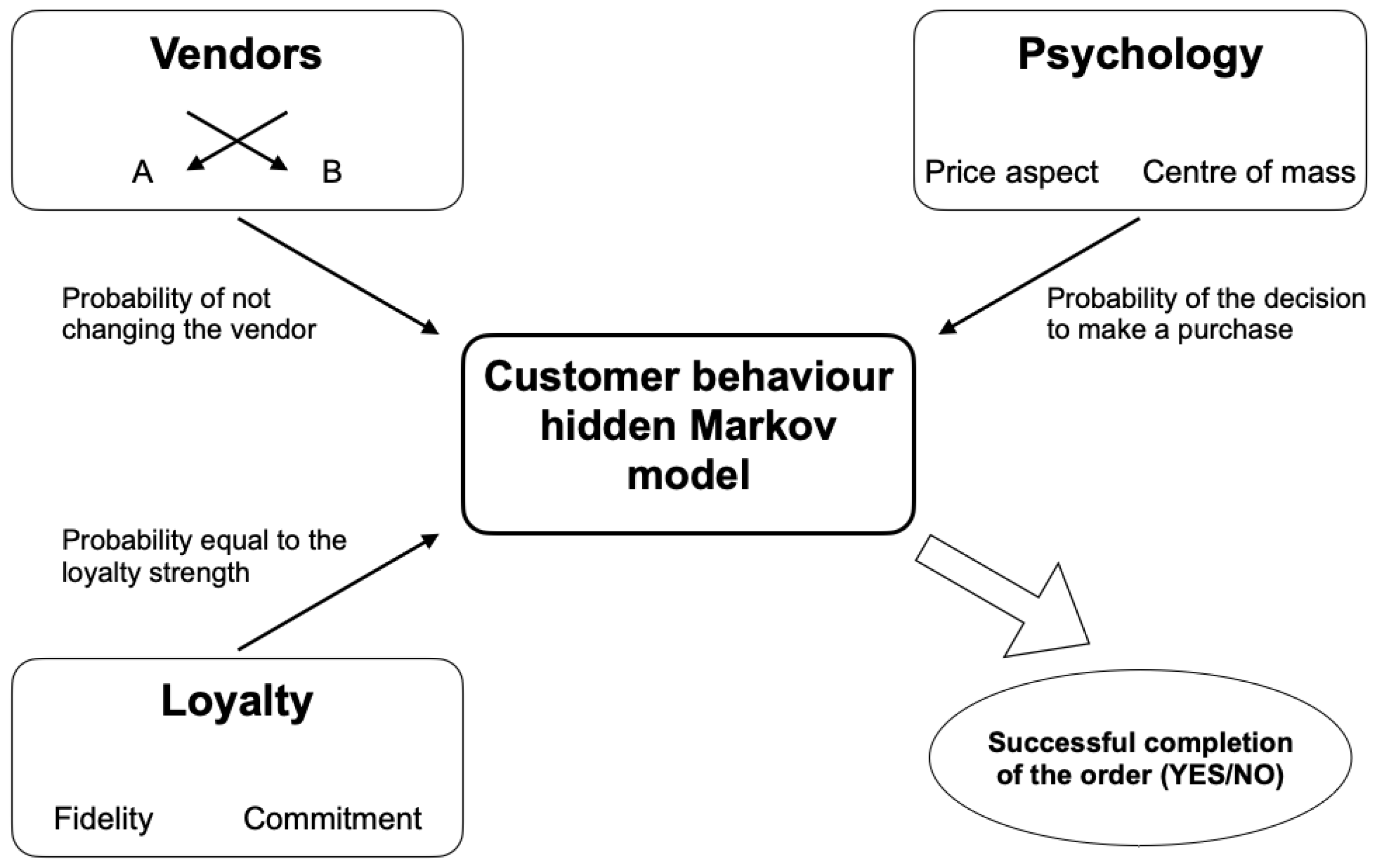
Let us propose a mathematical model performing the customer’s behaviour prediction, consisting of three sub-models: Vendor, Psychology and Loyalty, that are used in the transition matrix of hidden Markov models (see Figure 1). The proposed customer behaviour hidden Markov model (CBHMM) returns a prediction of a customer’s decision, i.e., whether or not an order in the store will be completed or not. Running it in cycles (for multiple customers), the number of predicted orders is obtained, that is further used to estimate the income of the store for a chosen time period. The CBHMM uses open data and Google Analytics data as the source for computing the model parameters.

3.1. Vendors Sub-Model

For simplification, only two vendors’ market shares are taken into account, without 100% domination, because in a real market a 100% monopole is unlikely to be seen. Moreover, it would affect the sub-model by giving a false-positive result [20]. This model returns the probability of the customer’s decision to stay with the vendor A and not to change to vendor B. It is in the interval $[0, 1]$, where 0 means changing to vendor B (the customer leaves the store A), resulting in not completing the order, and where 1 means staying with the vendor A but it does not automatically mean the completion of the order, thus having this probability non-zero is necessary but not sufficient condition of the order completion.

The Vendors sub-model is based on the relation:

$$\begin{array}{c}\hfill p\left(\mathrm{V}\right)=\beta H(I_P\left(A\right)-I_P\left(B\right))+\gamma H(I_Q\left(A\right)-I_Q\left(B\right))\\ \hfill +\delta H(I_P\left(A\right)-I_P\left(B\right))H(I_Q\left(A\right)-I_Q\left(B\right)),\\ \hfill \beta ,\gamma ,\delta \in [0, 1],\beta +\gamma +\delta \le 1,\end{array}$$

(3)

where $\beta$, $\gamma$, and $\delta$ are weighting factors that are dependent on the usual behaviour of customers in the specific industry field, $I_P$ is the price index of the vendor’s product, $I_Q$ is the quality index of the vendor, and H is the Heaviside function, having values:

$$\begin{array}{c}\hfill H\left(\arg \right)=1,\arg >0,\\ \hfill H\left(\arg \right)=0,\arg \le 0.\end{array}$$

(4)

3.2. Psychology Sub-Model

The psychology aspect simulates customer’s behaviour in situations, when the customer is influenced e.g., by price effect, society pressure, mood aspect, mass effect, actual needs, etc. In the proposed CBHMM the psychology sub-model is for simplification represented only by the price aspect (PA) and the centre of mass effect (CME), and in general, it represents the probability of a customer’s decision to make a purchase. It is in the interval $[0, 1]$, where 0 represents the decision that the purchase will not be made (not in the actual store nor elsewhere), and 1 represents the decision of the customer to realise the purchase, but not necessarily in the actual store, thus having this probability non-zero is necessary but not sufficient condition of the order completion.

The psychology sub-model is represented by the following probability:

$$\begin{array}{c}\hfill p\left(\mathrm{PS}\right)=\min \{\mathrm{PA}+\mathrm{CME};1\}.\end{array}$$

(5)

The price aspect can be represented by the “perception of store” index, that can be expressed as:

$$\mathrm{PA}=\frac{O_j\left(i\right)}{O\left(i\right)},$$

(6)

where $O_j\left(i\right)$ is the number of orders of product j per day i and $O\left(i\right)$ is the number of all orders of all products on a specific day i.

The centre of mass effect involves the use of sociology within the psychology sub-model. Marketers use it to manipulate customers in a global way, e.g., by “sales” such as Black Friday, Cyber Monday, etc., during which the customer’s psychology is manipulated by discount prices. The centre of mass effect can be represented by the “price psychology” index, expressed as [22]:

$$\mathrm{CME}=\frac{\max \{{\mathrm{PI}}_j,\stackrel{-}{P}\}}{\max \{P_j,\stackrel{-}{P}\}},$$

(7)

where $P_j$ is the price of the selected product j the customer is interested in, ${\mathrm{PI}}_j$ is the product index of the selected product j, which is computed as the retail recommended price (RP_j) minus the product price:

$${\mathrm{PI}}_j={\mathrm{RP}}_j-P_j,$$

(8)

and $\stackrel{-}{P}$ can be computed as:

$$\stackrel{-}{P}=\frac{1}{n_p}\sum _{j=1}^{n_p}{\mathrm{PI}}_j,$$

(9)

where $n_p$ is the number of all products in the store.

3.3. Loyalty Sub-Model

The Loyalty sub-model represents the customer’s positive feelings towards the store, and thus their dedication to make a purchase there. It is composed of two main components: Fidelity and Commitment, and can be represented by the relation:

$$p\left(\mathrm{L}\right)=\min \left\{\frac{p\left(\mathrm{F}\right)+p\left(\mathrm{C}\right)}{p\left(\mathrm{C}\right)};1\right\},$$

(10)

where $p\left(\mathrm{L}\right)$ is the probability of the Loyalty sub-model, $p\left(\mathrm{F}\right)$ is the probability of the Fidelity component, and $p\left(\mathrm{C}\right)$ is the probability of the Commitment component (that has to be formally non-zero).

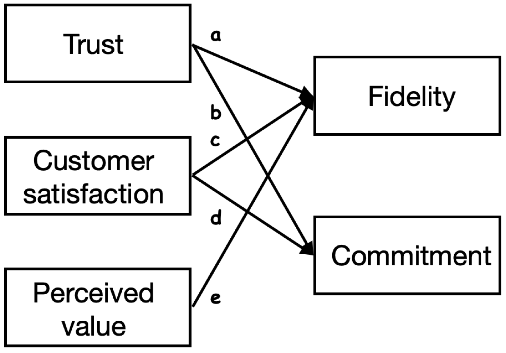
Similarly to [23], we compute the Fidelity and Commitment components as a linear combination of Trust (T) and Perceived value ($\mathrm{PV}$) that can be computed from the Google Analytics data, and from the customer satisfaction ($\mathrm{CS}$) that can be obtained from the open data (Figure 2). The term CS represents the average satisfaction with the store, and PV depends on the strength of the store. Both are in the interval $[0, 1]$. Trust, that represents the customer’s confidence with the store, can be defined as:

$$\mathrm{T}=\min \left\{\frac{O\left(i\right)}{V\left(i\right)};1\right\},$$

(11)

where $O\left(i\right)$ is the number of all orders of all products, and $V\left(i\right)$ is the number of visitors on a specific day i.

The partial probabilities are then evaluated using the following relations:

$$\begin{array}{c}\hfill p\left(\mathrm{F}\right)=a\mathrm{T}+c\mathrm{CS}+e\mathrm{PV},\\ \hfill p\left(\mathrm{C}\right)=b\mathrm{T}+d\mathrm{CS},\\ \hfill \mathrm{where}a+c+e\le 1\mathrm{and}b+d\le 1,\end{array}$$

(12)

and where $a, b, c, d, e\in [0, 1]$ are weights that are also computed from the open data.

3.4. The CBHMM Decision Process

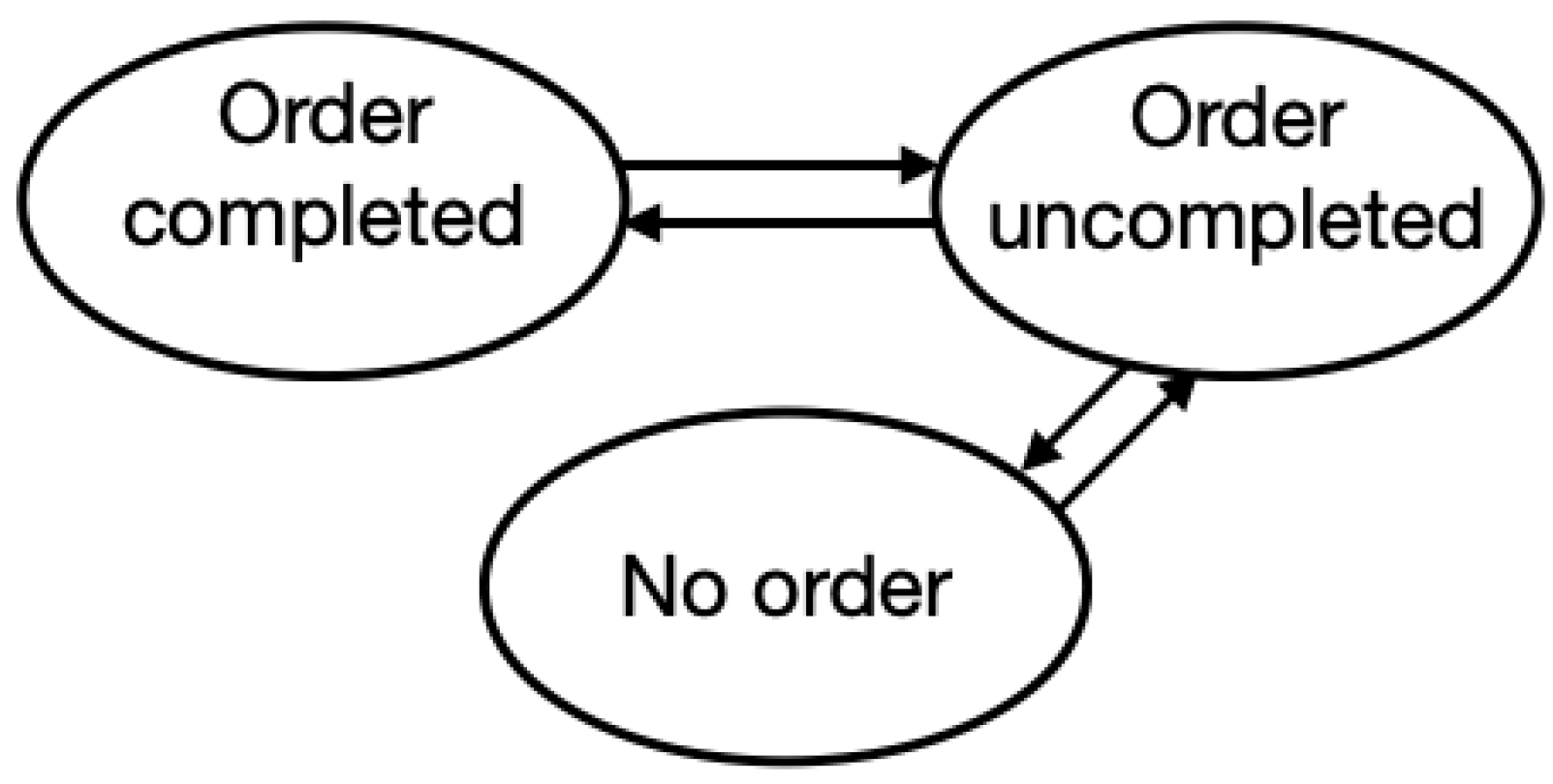
The probabilities returned by the Vendors, Psychology and Loyalty sub-models are used by the proposed customer behaviour hidden Markov model (CBHMM) with the goal to predict the customer’s decision if an order will be completed or not. The three sub-models correspond to the three states “Order completed”, “Order uncompleted”, “No order” (see Figure 3), where the Vendors sub-model is linked to the state “Order completed”, Psychology sub-model represents the state “Order uncompleted”, and Loyalty sub-model represents the “No order” state. This premise is based on marketing principles and the affinity between the states and the sub-models.

The CBHMM simulates customers’ behaviour during the ordering process. First, the decision sequence using three states: “Order completed”, “Order uncompleted”, “No order” is estimated by solving the relation:

$$\begin{array}{c}\hfill P\left(A|E\right)=p\left(\left(\begin{array}{ccc}p\left(\mathrm{V}\right)& p\left(\mathrm{PS}\right)& p\left(\mathrm{L}\right)\end{array}\right)|\left(\begin{array}{ccc}l& m& k\end{array}\right)\right),\end{array}$$

(13)

where $P\left(V\right)$ is the vendor probability, $p\left(\mathrm{PS}\right)$ is the psychology model probability, $p\left(\mathrm{L}\right)$ is the loyalty model probability, all of them forming the transition matrix A, and where $l,m,k$ are initial probabilities of the three states, “Order completed”, “Order uncompleted”, “No order”, forming the emission matrix E.

The outputting sequence $P\left(A|E\right)$ represents the three states sorted decreasingly based on the highest probability. Afterwards, the decision sequence is read and decoded by the Viterbi algorithm to estimate the “path” through the sequence, thus the sequence is rearranged to estimate “what happens first”. The final result of the CBHMM (if the order will be completed or not) depends on the fulfilment of the condition if the state “Order completed” is in front of the state “No order” in the rearranged sequence.

4. Numerical Experiment

This work is focused on the prediction of customer behaviour, with the goal to predict the income of a store for a chosen period of time. The proposed CBHMM was compared to the baseline prediction represented by the Google Analytics tracking system mechanism—the standard prediction used in e-commerce (further denoted as the GA model). Both models are using real anonymised data from a prior time period as the input. Based on these data, specific parameters are computed, that are then used for income forecasting. Thus, due to making the models “applicable” for real practical prediction, neither of them is using parametrical optimisation.

4.1. Prediction Models

The GA model that is used in this work as the baseline, uses standard computation of the prediction of income in the form:

$${\mathrm{Income}}_{\mathrm{GA}}=v·AV·CR,$$

where v is the predicted number of visitors, $AV$ is the predicted average order value, and $CR$ is the conversion rate, which can be expressed as the ratio between the number of orders and the number of visitors. All three variables: v, $AV$ and $CR$ are estimated from the real prior data tracked from the store.

In case of using CBHMM, the income of the business can be predicted based on the relation:

$${\mathrm{Income}}_{\mathrm{CBHMM}}=PO·AV,$$

(14)

where $PO$ is the predicted number of orders obtained from CBHMM, and $AV$ is the predicted average order value from the prior data gained using the GA mechanism (which is the same as in the previous model).

4.2. Comparison Criteria

Two quality measures were used to compare the performance of the models. The first of them is the R-squared, a statistical measure of fit that indicates how much variation of a dependent variable is explained by the independent variable in the model, in other words, it shows how well terms (data points) fit a curve or a line. R-squared is returning a value from interval $[0, 1]$, where 1 means that all dependent variables are completely explained by the independent variables (a perfect fit). The R-squared can be defined as the ratio between the sum of squared errors ($SSE$) and the sum of squared total ($SST$):

$$R^2=1-\frac{SSE}{SST},$$

where $SST$ expresses the squared differences between the observed dependent variable and its mean $SST={\sum }_{i=1}^n{(y_i-\overline{y})}^2$, and where $SSE$ can be defined as the difference between the observed value and the predicted value: $SSE={\sum }_{i=1}^n{(y_i-\widehat{y_i})}^2$, with values of $SSE$ closer to 0 indicating a smaller random error component of the model.

The second performance measure is the prediction gain ($PG$), defined as the logarithm of the power ratio of the observed value and the resulting error between the actual values y and the predicted values $e=y-\widehat{y}$:

$$PG\left[\mathrm{dB}\right]=10{\log }_{10}\frac{y^2}{e^2}.$$

The lower is the error e, the higher the prediction gain.

4.3. Results and Discussion

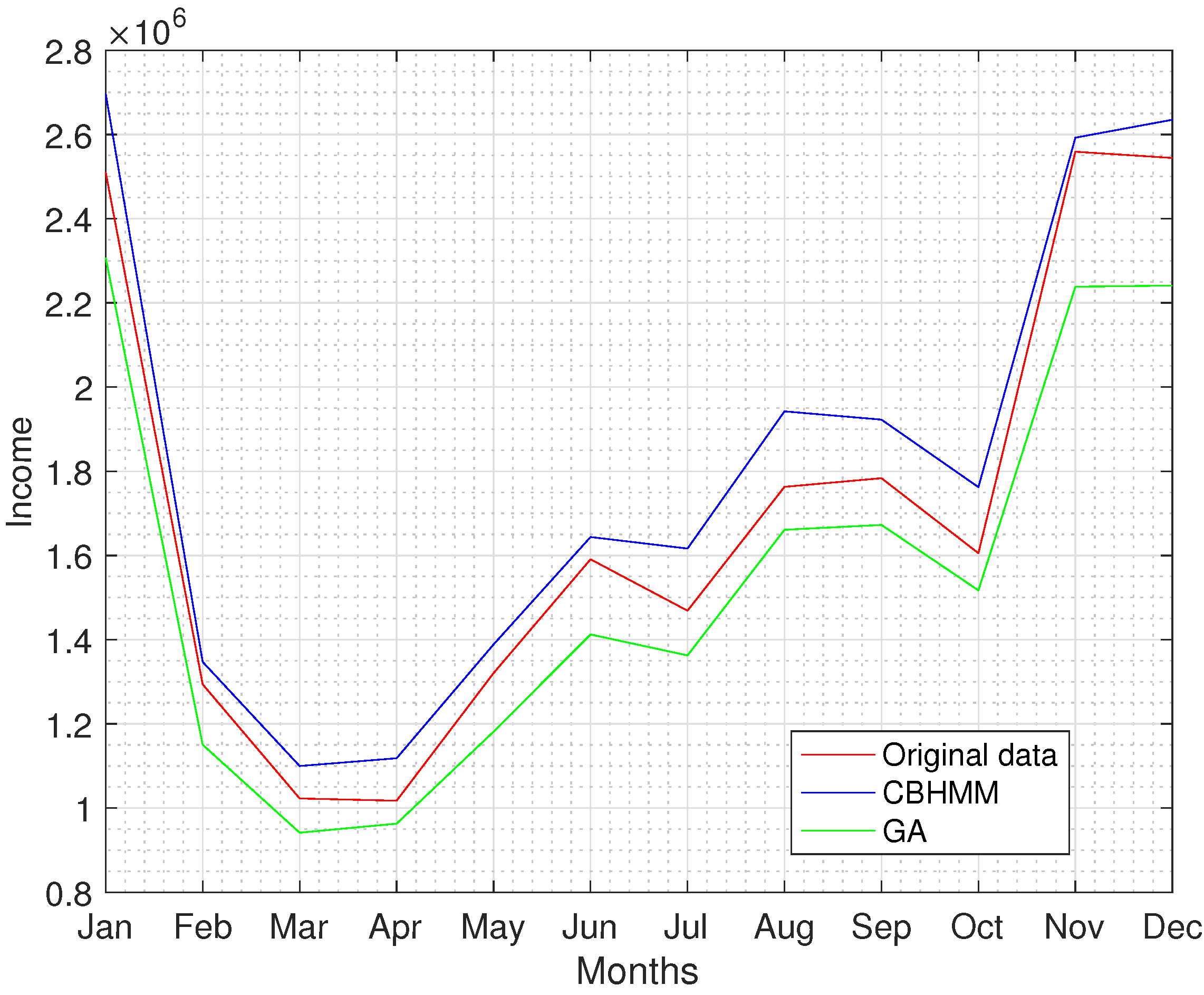
The GA model, as well as the CBHMM, were used to compute the income of a store under study, for the year 2021, where the input was in the form of real data from three previous years (2018–2020) from Google Analytics as well as open data. The prediction results were compared to original data where the R-squared and $PG$ performance measures were used as the quality criteria for comparison of the two models.

From Figure 4 it is possible to observe that the prediction of income evaluated by both models is copying the trend of real income data obtained from the store, demonstrating that both methods are relevant to predicting the income of stores.

Moreover, the results of the store income forecast are presented in the form of a table, where the real income for the year 2021, the aberration in prediction using the GA model and the CBHMM, and the difference between the two compared models are given (see

Table 1. Real income and aberration in prediction of income using the GA model and CBHMM for the year 2021.

2021 Month	Real Income	GA Model Aberration [%]	CBHMM Aberration [%]	Models Difference [%]
January	2,510,086.00	−8.10	7.43	15.53
February	1,293,778.00	−11.09	4.12	15.22
March	1,022,762.00	−7.94	7.54	15.48
April	1,017,408.00	−5.36	9.91	15.28
May	1,320,608.00	−10.54	5.15	15.69
June	1,590,878.00	−11.22	3.33	14.55
July	1,468,808.00	−7.23	10.05	17.28
August	1,762,959.00	−5.78	10.17	15.95
September	1,783,582.00	−6.22	7.80	14.02
October	1,605,396.00	−5.50	9.77	15.27
November	2,559,070.00	−12.53	1.30	13.84
December	2,544,271.00	−11.99	3.57	15.48

).

There are several interesting facts, that can be concluded from the results given in Table 1. The GA model was predicting the income for all 12 months of the observed period lower than it finally was. On the other hand, the CBHMM was predicting the income always be greater (in the case of all 12 months) than the real income. Another very interesting observation is, that the difference between the two compared models is almost constant for the whole period under study, thus the proposed CBHMM is copying the trend of real data at least as good as the GA model, which can be thought of as the baseline model in e-commerce.

The models were also compared using two comparison criteria, the $R^2$ and $PG$ (see

Table 2. Prediction performance using the GA model and CBHMM for the year 2021.

	GA Model	CBHMM
$R^2$	0.90	0.95
$PG$	20.29	23.45

). Both criteria are in favour of the proposed CBHMM, resulting in a fit 5% better than the GA model, from the viewpoint of $R^2$, and CBHMM outperforms the GA model in terms of $PG$ more than 3 dB better.

5. Conclusions

In this work, a mathematical model, that predicts customer’s behaviour during the ordering process, is proposed with the goal to predict the income of a store for a chosen period of time. The proposed customer behaviour hidden Markov model (CBHMM) is composed of three sub-models, Vendors, Psychology and Loyalty, that are linked with the three states “Order completed”, “Order uncompleted”, “No order”. The hidden Markov model is used to compute the decision sequence, sorting the three states decreasingly based on the highest probability, followed by the Viterbi algorithm that estimates the “path” through the sequence, thus rearranging the sequence with the goal to estimate what happens first, “Order completed” or “No order”. The CBHMM was compared to the baseline prediction represented by a GA model that uses the Google Analytics tracking system mechanism—the standard prediction used in e-commerce, using real anonymised prior data from previous years (2018–2020) from Google Analytics as well as open data as the input. The predicted income computed using both models, CBHMM as well as GA model, was copying the trend of real income data obtained from the store, demonstrating that both methods are relevant to predicting the income of stores. Moreover, the distance between the two compared models was almost constant for the whole period under study, proving the applicability of the proposed CBHMM by the prediction of income. Furthermore, based on the $R^2$ and $PG$ comparison criteria evaluated on prediction results for the year 2021, both criteria were in favour of the proposed CBHMM, thus the CBHMM is fully applicable for customers’ behaviour prediction in e-commerce.

References

- Abbasimehr, H.; Shabani, M. A new framework for predicting customer behavior in terms of RFM by considering the temporal aspect based on time series techniques. J. Ambient. Intell. Humaniz. Comput. 2021, 12, 515–531. [Google Scholar] [CrossRef]
- Badea, L.M. Predicting Consumer Behavior with Artificial Neural Networks. Procedia Econ. Financ. 2014, 15, 238–246. [Google Scholar] [CrossRef] [Green Version]
- Jing, L.; Shuxiao, P.; Lei, H.; Xin, Z. A Machine Learning Based Method for Customer Behavior Prediction. Teh. Vjesn.-Tech. Gaz. 2019, 16, 1670–1676. [Google Scholar]
- Martinez, A.; Schmuck, C.; Pereverzyev, S.; Pirker, C.; Haltmeier, M. A machine learning framework for customer purchase prediction in the non-contractual setting. Eur. J. Oper. Res. 2020, 281, 588–596. [Google Scholar] [CrossRef]
- Li, D.; Zhao, G.; Wang, Z.; Ma, W.; Liu, Y. A Method of Purchase Prediction Based on User Behavior Log. In Proceedings of the 2015 IEEE International Conference on Data Mining Workshop (ICDMW), Atlantic City, NJ, USA, 14–17 November 2015; pp. 1031–1039. [Google Scholar]
- Bell, D.; Mgbemena, C. Data-driven agent-based exploration of customer behavior. Simulation 2018, 94, 195–212. [Google Scholar] [CrossRef] [Green Version]
- Dakduk, S.; Horst, E.T.; Santalla, Z.; Molina, G.; Malavé, J. Customer Behavior in Electronic Commerce: A Bayesian Approach. J. Theor. Appl. Electron. Commer. Res. 2017, 12, 1–20. [Google Scholar] [CrossRef] [Green Version]
- Boyer, K.K.; Hult, G. Customer Behavior in an online ordering application: A decision scoring model. Decis. Sci. 2005, 36, 569–598. [Google Scholar] [CrossRef]
- Hernandez, B.; Jimenez, J.; Martin, M.J. Customer behavior in electronic commerce: The moderating effect of e-purchasing experience. J. Bus. Res. 2010, 63, 964–971. [Google Scholar] [CrossRef]
- Peentland, A.; Liu, A. Modeling and Prediction of Human Behavior. Neural Comput. 1999, 11, 220–240. [Google Scholar] [CrossRef] [PubMed]
- Forney, G.D. Viterbi algorithm. Proc. IEEE 1973, 61, 268–278. [Google Scholar] [CrossRef]
- Forney, G.D., Jr. The Viterbi Algorithm: A personal history. arXiv 2005, arXiv:cs/0504020. [Google Scholar]
- Xiao, S.S.; Dong, M. Hidden semi-Markov model-based reputation management system for online to offline (020) e-commerce markets. Decis. Support Syst. 2015, 77, 87–99. [Google Scholar] [CrossRef]
- Hassan, M.R.; Nath, B.; Kirley, M. A fusion model of HMM, ANN and GA for stock market forecasting. Expert Syst. Appl. 2007, 33, 171–180. [Google Scholar] [CrossRef]
- Srivastava, A.; Kundu, A.; Sural, S.; Majumdar, A.K. Credit card fraud detection using hidden Markov model. IEEE Trans. Dependable Secur. Comput. 2008, 5, 37–48. [Google Scholar] [CrossRef]
- Mamata, J.; Pratap, K.J.; Mohapatra, S.G. A stochastic model of e-customer behavior. Electron. Commer. Res. Appl. 2003, 2, 81–94. [Google Scholar]
- Kakalejcik, L.; Bucko, J.; Vajecka, M. Differences in Buyer Journey between High- and Low-Value Customers of E-Commerce Business. J. Theor. Appl. Electron. Commer. Res. 2019, 14, 81–94. [Google Scholar] [CrossRef] [Green Version]
- Chang, L.; Ouzrout, Y.; Nongaillard, A.; Bouras, A.; Jiliu, Z. The Reputation Evaluation Based on Optimized Hidden Markov Model in E-Commerce. Math. Probl. Eng. 2013, 2013, 391720. [Google Scholar] [CrossRef]
- Liberali, G.; Ferecatu, A. Morphing for Consumer Dynamics: Bandits Meet Hidden Markov Models. Mark. Sci. 2022. ahead of print. [Google Scholar] [CrossRef]
- Patel, S.; Schlijper, A. Models of Consumer Behaviour; Unilever Corporate Research: London, UK, 2016. [Google Scholar]
- Shai, F.; Singer, Y.; Tishby, N. The Hierarchical Hidden Markov Model: Analysis and Applications. Mach. Learn. 1998, 32, 41–62. [Google Scholar]
- Willsky, A.S. Detection of Abrupt Changes in Dynamic Systems; Springer: Berlin/Heidelberg, Germany, 1986; pp. 154–196. [Google Scholar]
- Luarn, P.; Lin, H.H. A customer loyalty model for e-service context. J. Electron. Commer. Res. 2003, 4, 156–167. [Google Scholar]
Figure 1.
The structure of the Customer behaviour hidden Markov model.
Figure 2.
Composition of the Fidelity and Commitment components.
Figure 3.
Sequence of possible states.
Figure 4.
Prediction of income using the CBHMM and GA models, in comparison to real income for the year 2021.