Article

Impact of Third-Degree Price Discrimination on Welfare under the Asymmetric Price Game

1
School of Management Science and Engineering, Shandong University of Finance and Economics, Jinan 250014, China
2
School of Business, Renmin University of China, Beijing 100872, China
3
School of Management, Shandong University, Jinan 250100, China
*
Author to whom correspondence should be addressed.
Mathematics 2022, 10(8), 1215; https://doi.org/10.3390/math10081215
Submission received: 9 February 2022 / Revised: 29 March 2022 / Accepted: 4 April 2022 / Published: 7 April 2022
(This article belongs to the Topic Game Theory and Applications)

Abstract

:
Whether third-degree price discrimination improves or damages social welfare has always been a hot topic for scholars of economics. At present, research studies on the impact of third-degree price discrimination on welfare have not been carried out under asymmetric price competition. To this end, we studied this problem. In the research process, we divided consumers into two market segments by setting different travel costs based on the Hotelling model; at the same time, we considered three scenarios in which both firms engage in uniform pricing, both engage in price discrimination, and price discrimination vs. uniform pricing, and some intriguing findings and conclusions that differ from the previous studies were obtained through game analysis: (1) compared with two symmetric price games, the total output effect of each firm is unchanged, but the total social welfare is reduced, and as the size of the strong market increases, the reduction effect of total social welfare increases first and then decreases; (2) from local social welfare analysis, although the output of the firm adopting price discrimination remains unchanged, it can produce more producer surplus, consumer surplus and social welfare third-degree; (3) while the firm that uses uniform pricing is at a disadvantage in competition, the local social welfare created by it is decreased, and the reduction effect of social welfare will increase first and then decrease as the increase of the size of the strong market occurs. These conclusions reveal in an oligopoly market why enterprises always choose price discrimination and the government acquiesces in the existence of price discrimination.

1. Introduction

In real society, to obtain higher profits, enterprises often carry out differentiated pricing according to the different market segments, which is called third-degree price discrimination in economics [1]. For example, airlines and travel agencies offer the same services at different rates for different groups of people, such as children, students and adults. In addition, in telecommunications charges, electricity pricing, and other fields, oligarchic enterprises’ use of discrimination is very common. Interestingly, in these monopolistic industries, none of the enterprises will give up price discrimination and choose a uniform pricing strategy. In addition, although the government has been insisting on anti-monopoly, such price discrimination is not prohibited and has even become the business rule under government regulation. What causes this phenomenon? Is it impossible for enterprises to gain a competitive advantage by adopting a uniform pricing strategy in an oligopoly market? Can social welfare not be improved when firms choose to compete at flat prices? This has triggered us to find out the answers.
Although there is sufficient literature to help us study these kinds of problems, most of them are studied under situations of a monopoly or symmetric price game, and the lack of asymmetric price competition situations with uniform pricing versus price discrimination among firms, so these problems cannot be fully explained. Therefore, in order to explain these problems explicitly, we analyze the relationship between third-degree price discrimination and social welfare under the asymmetric price game.
We used Askar, S. et al.’s analytical paradigm for reference [2] and analyzed the relationship between third-degree price discrimination and social welfare from the global and local aspects under an asymmetric price game. Meanwhile, considering the market structure of price discrimination conducted by firms generally includes strong markets and weak markets. According to Robinson, a strong market is one in which firms can sell at a high price, and a weak market is one in which firms can only sell at low prices [3]. In this paper, therefore, so as to better describe market segmentation and consumption market structure, we refer to the model processing and setting ideas of literature [4], and take the original Hotelling model as the basis, by setting two kinds of travel costs to divide the two types of consumers, and by setting appropriate parameters to represent the proportion of the two types of consumer groups in the market. Then, we use this improved model to analyze the impact of third-degree price discrimination on social welfare. Compared to other models, using the improved Hotelling model can not only reflect the enterprise’s market monopoly scope, but also accurately describe the different consumers’ groups and sizes in the market (Compared with the traditional Betrand game model, the Hotelling model considers the location monopoly power of enterprises; it effectively avoids the Betrand paradox, and makes the research more meaningful. Meanwhile, different from the vertical differentiation model, we still retain the characteristics of the two enterprises producing homogeneous products, which can reduce the impact of product quality differentiation).
In this study, the following research questions were investigated: first, under the asymmetric price game, does the total social welfare increase, decrease, or remain the same? Second, from the perspective of local social welfare, what happens to producer surplus, consumer surplus, and social welfare created by firms with different pricing strategies? Finally, what are the effects of changes in market structure on total social welfare and local social welfare?
We extend the findings of existing literature. Compared with two symmetric price games, in the asymmetric price game, the total social welfare decreases, and the reduction effect of the total social welfare increases first and then decreases with the strong market size increases. In the local market, although the output of the firm adopting price discrimination remained unchanged, it can produce more producer surplus, consumer surplus and social welfare. While firms that adopt uniform pricing will reduce local social welfare, the reduction effect of social welfare will increase and then decrease as the strong market size increases. The in-depth discussion of this topic helps us recognize the relationship between third-degree price discrimination and social welfare, which guides firms to make price decisions and helps the government to take effective measures and activities to improve social welfare.
The rest of the paper is organized as follows. A brief review of the related research paper is presented in Section 2. In Section 3, we set up three game models under the conditions of uniform pricing for both firms, price discrimination for both firms, and price discrimination vs. uniform pricing. In Section 4, we analyze the equilibrium values of the three situations and get relevant propositions. In Section 5, the results are simulated and analyzed numerically. Section 6 concludes the paper. In addition, some important proofs are presented in Appendix A.

2. Literature Review

Our analysis is related to the literature on third-degree price discrimination in oligopolistic markets under differentiated competition.
Third-degree price discrimination is a way for firms to gain profits by snatching consumer surplus [5,6]. Initially, studies on third-degree price discrimination were conducted under the assumption of perfect monopoly [7]. On this basis, Adams, C.F. (2019) found that firms could create greater monopoly profits and efficiency losses by considering quality choices and monopoly power [8]. Wang, X. and Zhang, L. (2021) found that monopolistic downstream third-degree price discrimination increases social welfare when input prices are determined by suppliers by reconsidering the effects of a monopolistic aspect in a vertical market [9].
However, in real society, the real monopoly manufacturers almost do not exist, there are only oligarchs with certain monopoly ability in the market. In an oligopolistic market, because each oligopolistic firm competes with each other, the game of pricing strategy between them will affect the competitive equilibrium, so the third-degree price discrimination does not necessarily meet the welfare judgment standard of a monopolistic market. Therefore, the study of third-degree price discrimination has been extended to oligopolistic markets, where the effects of third-degree price discrimination on firms and consumers are more complex due to competitive effects, which may increase or decrease total output, firm profit, consumer surplus, and social welfare [10,11]. For example, Miklós-Thal, J. and Shaffer, G. (2019) considered input costs on the basis of existing research and found that, when competition in strong markets is more intense than in weak ones, making price discrimination is less likely to increase total output [12]. Aguirre, I. (2019) found that, under oligopoly price discrimination, compared with the demand slope, the total output effect is more easily affected by the number of firms [13].
However, the above research does not consider the differentiated competitive behavior of enterprises. In economic activities, the competitive behavior among enterprises will not be completely consistent. Therefore, some scholars have extended the research scope of three-level price discrimination to the field of differentiated competition based on this research, such as the Armstrong and Vickers (2001) study, a discrete choice model with symmetric firms. If one firm’s strong market is another firm’s weak market, price discrimination in such asymmetric competition will benefit consumers and harm duopoly firms [14]. Unlike pure price discrimination, Chen and Schwartz (2012) studied the welfare effect of cost differential price discrimination considering that marginal costs also differ between markets, and found that, in the case of different sub-market costs, price discrimination will increase the total social welfare even if the total output does not increase, because the total output is more allocated to the low-cost market, and thus reduces the total social cost [15]. Adachi and Matsushima (2014) researched the welfare effects of oligopolistic price discrimination with horizontal product differentiation and found that the condition for third-degree price discrimination to improve the total social welfare is that the product substitution degree of the strong market must be significantly higher than that of the weak market [16]. Galera et al., (2017) analyzed the impact of price discrimination on welfare in the presence of quality differences. They show that if the quality levels of the local firms’ products are the same, price discrimination always increases welfare, mainly because of a positive allocation effect of price discrimination [17]. Feng and Ma investigated (2018) how firms choose their level of product differentiation when engaging in third-degree price discrimination in a competitive product market; their results show that firms will only set themselves at the two end points to make their products as differentiated as possible if one group of consumers is sufficiently larger than the other [18]. Zhang, T. et al., (2019) considered location monopoly and found that price discrimination improves social welfare when demand elasticity is large enough [19]. Galera et al., (2019), assuming that preferences are not quasilinear, found that in the presence of consumer income differences, total consumer utility may increase under third-degree price discrimination, while total output remains constant [20]. Chung (2021) studied the welfare impacts of price discrimination when firms are asymmetric in quality improvement costs, and shows that price discrimination increases social welfare relative to uniform pricing if the firms’ cost gap is large enough [21].
Although there is sufficient literature to help us study this issue, how price discrimination affects firm profits, consumer surplus, and total social welfare under an asymmetric price game is under-researched. We thus extend existing research to the situation of asymmetric price games between firms and analyze the impact of third-degree price discrimination on social welfare under this situation.

3. The Model

3.1. Basic Model

In a duopoly market, firm 1 and firm 2 are located at the two ends of a linear city (0,1); it is assumed that firm 1 is at 0 and firm 2 at 1. The products produced by the two firms have no differences and the production cost is c. The two firms play the price game simultaneously.
There exist two groups of consumers, A, B, who are uniformly distributed in a linear city. The total consumer size is normalized to 1. We assume that the size of consumers in group A is b   and the size of consumers in group B is 1 b and each consumer buys only one unit of the product. Due to the above settings, the parameter b used to represent changes in market structure, the value of b increases, which means an increase in the proportion of consumers in group A and a decrease in the proportion of consumers in group B.
We consider and compare three price game situations among the firms, such as uniform pricing vs. uniform pricing denoted by superscript “uu”, where firm i, i = 1, 2, they compete with each other with uniform pricing, which charges the same price to the two groups of consumers. Under uniform pricing vs. discrimination pricing denoted by superscript “dd”, both firms compete using price discrimination, which charges the different prices to the two groups of consumers. Under discrimination pricing vs. uniform pricing denoted by superscript “ud”, in this competition, one firm uses price discrimination, and another firm adopts uniform pricing. We assume that firm 1 charges different prices to the two types of consumers, but firm 2 charges the same price to the two types of consumers. Then, we use superscripts including “uu”, “dd”, and “ud” to indicate the three situations of price competition among firms and subscript including “1” and “2” to index the firm members throughout this paper.
In terms of model setup, we refer to the settings on consumer differences of Yl and Jie [22]. For a consumer in group j, for j = A, B, located at x, if she buys the product from firm i, her utility is:
U i j = V p i j x i t j
where V is the utility obtained by the consumer from the purchase of the product and V is large enough to allow the market to be fully covered. p i j is the price charged to the consumers in group j by firm i, t j is the unit transportation cost for consumers in group j, and x j the distance between the consumer and firm i. Because the cost of travel differs between the two types of consumers, without loss of generality, we assume that t A > t B . For the firms, high-travel-cost consumers mean that this can bring high-product pricing to the firms. In other words, consumers in group A is a strong market for firms, and consumers in group B is a weak market for firms.
Let u 1 j = u 2 j . It follows that x ¯ j = p 2 j p 1 j + t j 2 t j . Consumers in group j at location x ¯ j get the same utility from purchasing a product from either firm 1 or firm 2. Therefore, the demand functions for the two firms are:
q 1 = q 1 A + q 1 B = b x ¯ A + ( 1 b ) x ¯ B  
q 2 = q 2 A + q 2 B = b ( 1 x ¯ A ) + ( 1 b ) ( 1 x ¯ B )  
At this point, the profits of the two firms are:
π 1 = j = A , B ( p 1 j c ) q 1 j
π 2 = j = A , B ( p 2 j c ) q 2 j
Consumer surplus in the market governed by firm i   ( i = 1 , 2 ) is equal to the sum of the utilities obtained by different types of consumers purchasing products from firm i   ( i = 1 , 2 ) :
C S 1 = b 0 x ¯ A U 1 A d x + ( 1 b ) 0 x ¯ B U 1 B d x
C S 2 = b x ¯ A 1 U 2 A d x + ( 1 b ) x ¯ B 1 U 2 B d x
After simplification, we get:
C S 1 = V ( q 1 A + q 1 B ) q 1 A 2 t A 2 b q 1 B 2 t B 2 ( 1 b ) p 1 ( q 1 A + q 1 B )
C S 2 = V ( q 2 A + q 2 B ) q 2 A 2 t A 2 b q 2 B 2 t B 2 ( 1 b ) p 2 ( q 2 A + q 2 B )
Total consumer surplus is then equal to the sum of consumer surplus in the market under the jurisdiction of each firm:
C S = V q 1 A 2 t A 2 b q 2 A 2 t A 2 b q 1 B 2 t B 2 ( 1 b ) q 2 B 2 t B 2 ( 1 b ) p 1 ( q 1 A + q 1 B ) p 2 ( q 2 A + q 2 B )
Social welfare in the market governed by firm i   ( i = 1 , 2 ) is equal to the sum of consumer surplus in the market governed by firm i   ( i = 1 , 2 )   and profit of firm i   ( i = 1 , 2 ) :
S W 1 = ( V c ) ( q 1 A + q 1 B ) q 1 A 2 t A 2 b q 1 B 2 t B 2 ( 1 b )
S W 2 = ( V c ) ( q 2 A + q 2 B ) q 2 A 2 t A 2 b q 2 B 2 t B 2 ( 1 b )
Total social welfare is the sum of social welfare in the market under the jurisdiction of each firm:
S W = V c q 1 A 2 t A 2 b q 2 A 2 t A 2 b q 1 B 2 t B 2 ( 1 b ) q 2 B 2 t B 2 ( 1 b )
Assuming that the information of two firms is completely symmetrical, they make price decisions simultaneously according to the maximization of their own interests.

3.2. Model Solution

(1) 
Under uniform pricing vs. uniform pricing
In the “uu” situation, each firm sells products to both types of consumers at the same price, and their equilibrium prices are as follows:
p 1 u u = p 2 u u = t A t B t B b + t A ( 1 b ) + c
From the equilibrium price, the equilibrium sales volume can be obtained:
q 1 A u u = q 2 A u u = b / 2 ,
q 1 B u = q 2 B u = ( 1 b ) / 2
The profit of each firm, consumer surplus, and social welfare in the market under its jurisdiction are as follows:
π 1 u u = π 2 u u = t A t B 2 [ t B b + t A ( 1 b ) ]
C S 1 u u = C S 2 u u = ( V c ) 2 b t A + ( 1 b ) t B 8 t A t B 2 [ t B b + t A ( 1 b ) ]
S W 1 u u = S W 1 u u = V c 2 b t A + ( 1 b ) t B 8
The total consumer surplus and total social welfare are:
C S u u = ( V c ) b t A + ( 1 b ) t B 4 t A t B t B b + t A ( 1 b )
S W u u = V c b t A + ( 1 b ) t B 4
(2) 
Under price discrimination vs. price discrimination
In the “dd” situation, both firms sell products at different prices for two groups of consumers, and their equilibrium prices are:
p 1 A d d = p 2 A d d = t A + c
p 1 B d d = p 2 B d d = t B + c
From the equilibrium price, the equilibrium sales volume can be obtained:
q 1 A d d = q 2 A d d = b / 2
q 1 B d d = q 2 B d d = ( 1 b ) / 2
The profit of each firm, consumer surplus, and social welfare in the market under its jurisdiction are:
π 1 d d = π 2 d d = b t A + ( 1 b ) t B 2
C S 1 d d = C S 2 d d = V c 2 5 ( b t A + ( 1 b ) t B ) 8
S W 2 d d = S W 2 d d = V c 2 b t A + ( 1 b ) t B 8
The total consumer surplus and the total social welfare are, respectively:
C S d d = V c 5 ( b t A + ( 1 b ) t B ) 4
S W d d = V c b t A + ( 1 b ) t B 4
(3) 
Under price discrimination vs. uniform pricing
In the case of “ud” asymmetric price competition, it is assumed that firm 1 uses price discrimination and firm 2 conducts uniform pricing, and the two firms make price decisions simultaneously. Their equilibrium prices are:
p 1 A u d = t A 2 + t A t B 2 [ t B b + t A ( 1 b ) ] + c
p 1 B u d = t B 2 + t A t B 2 [ t B b + t A ( 1 b ) ] + c
p 2 u d = t A t B t B b + t A ( 1 b ) + c
From the equilibrium price, the equilibrium sales volume can be obtained:
q 1 A u d = b 4 ( 1 + t B t B b + t A ( 1 b ) )  
q 2 A u d = b 4 ( 3 t B t B b + t A ( 1 b ) )  
q 1 B u d = 1 b 4 ( 1 + t A t B b + t A ( 1 b ) )  
q 2 B u d 1 b 4 ( 3 t A t B b + t A ( 1 b ) )  
The profits of each firm, consumer surplus, and social welfare in the market under its jurisdiction are:
π 1 u d = b t A + ( 1 b ) t B 8 + 3 t A t B 8 [ t B b + t A ( 1 b ) ]  
π 2 u d = t A t B 2 [ t B b + t A ( 1 b ) ]  
C S 1 u d = V c 2 5 ( b t A + ( 1 b ) t B ) 32 15 t A t B 32 [ t B b + t A ( 1 b ) ]  
C S 2 u d = V c 2 9 ( b t A + ( 1 b ) t B ) 32 11 t A t B 32 [ t B b + t A ( 1 b ) ]  
S W 1 u d = V c 2 ( b t A + ( 1 b ) t B ) 32 3 t A t B 32 [ t B b + t A ( 1 b ) ]  
S W 2 u d = V c 2 9 ( b t A + ( 1 b ) t B ) 32 + 5 t A t B 32 [ t B b + t A ( 1 b ) ]  
The total consumer surplus and total social welfare are:
C S u d = V c 7 ( b t A + ( 1 b ) t B ) 16 13 t A t B 16 [ t B b + t A ( 1 b ) ]
S W u d = V c 5 [ b t A + ( 1 b ) t B ] 16 + t A t B 16 [ t B b + t A ( 1 b ) ]

4. Model Analysis

4.1. Total Social Welfare Analysis

By comparing the total output effect of each firm under different price game scenarios, we obtained the following propositions.
Proposition 1. 
q 1 d d = q 2 d d = q 1 u u = q 2 u u = q 1 u d = q 2 u d .
The proposition suggests that, in a fully covered duopoly competitive market, the total output of each firm is equal whether both firms engage in the “uu” situation, in the “dd” situation, or in the “ud” situation. That is, the total output of the firm using price discrimination will not decrease or increase because of different price game situations among firms.
Since the total output of each firm is equal in a fully covered duopoly market regardless of the game scenario, how do consumer surplus, producer surplus, and total social welfare change under different game scenarios? Proposition 2 can be obtained by comparing the total social welfare, consumer surplus, and producer surplus in each situation.
Proposition 2. 
(1) 
C S u u > C S u d > C S d d ;
(2) 
( π 1 d d + π 2 d d ) > ( π 1 u d + π 2 u d ) > ( π 1 u u + π 2 u u ) ;
(3) 
S W u u = S W d d > S W u d .
The proposition above suggests that, in a duopoly market with full coverage, whenever a firm uses price discrimination, it increases producer surplus and decreases consumer surplus, and producer surplus is highest and consumer surplus is lowest when both firms engage in price discrimination. However, the total social welfare is equal when both oligopolistic firms engage in uniform pricing or both engage in price discrimination, under the “ud” situation, the total social welfare is lower than the first two game scenarios.
From the formula of the total social welfare, the total social welfare function is related to the demand quantity of different types of consumers. In the symmetric price game, the demand of different types of consumers for the product remains unchanged, and it does not generate misallocation of consumption, that is, the total social welfare is equal under the “uu” or “dd” situation. Under the “ud” situation of such asymmetric price competition, although the total output of each firm does not change, the relative demand of each group of consumers changes, which leads to consumption misallocation, and thus to the reduction in social welfare.
This conclusion shows that price discrimination conducted by all firms does not hurt the total social welfare on the contrary, the total social welfare amounts are reduced when there is uniform pricing used by some firms in the market competition. That is why the government acquiesces firms to conduct price discrimination.
Lemma 1. 
(1) 
d S W u u d b = d S W d d d b < 0 ;
(2) 
d S W u d d b < 0 , when   b t A t A t B / 5 t A t B , d S W u d d b > 0 , when b > t A t A t B / 5 t A t B .
The proof of Lemma 1 can be found in Appendix A. This lemma shows that the total social welfare, as the size of the strong market increases, decreases under the “uu” or “dd” symmetric price games and decreases before increasing under the “ud” asymmetric price game.
Specifically, under the “uu” or “dd” situation of such symmetric price games, as the size of the strong market increases, total consumer surplus decreases faster than the increase in firm profits, which results in a decrease in total social welfare. In the “ud” situation of the asymmetric price game, due to misallocation of consumption, when the size of the strong market is small and that of the weak market is large, as the size of the strong market increases, the rate of decrease in total consumer surplus is higher than the rate of increase in total firm profits. When the size of the strong market increases above a certain threshold, the rate of decline of total consumer surplus is lower than the rate of increase of total profit. Therefore, total social welfare will decrease and then increase. From this lemma, we get the following proposition.
Proposition 3.
Under the asymmetric price game, the reduction effect of total social welfare increases when b t A t A t B t A t B , and then decreases when b > t A t A t B t A t B .
The proof of Proposition 3 can be found in Appendix A. Under the asymmetric price game, we find that the reduction effect of the total social welfare increases first and then decreases with the size of the strong market increases. This is because total social welfare will decrease and then increase. This conclusion shows that, when firms engage in asymmetric price competition, if the size of the strong market increases, the decline of the total social welfare does not increase monotonously all the time, but starts to decrease monotonously when it reaches a certain threshold. This indicates that, when such asymmetric price competition exists in the market, some reasonable actions taken by the government at the threshold point, urging relevant firms to change their price competition strategies (uniform pricing or price discrimination) and making all firms in the market adopt the same price competition strategy, will improve the total social welfare most obviously.

4.2. Local Social Welfare Analysis

To further clarify the increases or decreases in social welfare, from the local social welfare analysis, Proposition 4 can be obtained by comparing the local social welfare, local consumer surplus, and each firm’s profit in each situation.
Proposition 4. 
(1) 
  π 1 d d = π 2 d d > π 1 u d > π 2 u d = π 1 u u = π 2 u u ;
(2) 
C S 1 u u = C S 2 u u > C S 1 u d > C S 2 u d > C S 1 d d = C S 2 d d ;
(3) 
S W 1 u d > S W 1 d d = S W 1 u u = S W 2 d d = S W 2 u u > S W 2 u d .
Proposition 4 suggests that, under the asymmetric price game, the firm that chooses price discrimination generates higher profits than the one that adopts uniform pricing. At the same time, when both firms adopt price discrimination competition, the profit of the two firms is the highest; and when both firms adopt uniform pricing, the profit of the two firms is the lowest. Therefore, it is a dominant strategy for firms to practice third-degree price discrimination in a duopoly market with full coverage. In addition, the firm that uses price discrimination can generate more consumer surplus and local social welfare than the firm that uses uniform pricing. This further explains why the government acquiesces firms, such as airlines and power-supplied enterprises to conduct price discrimination.
This conclusion contrasts with that obtained in the case of a perfect monopoly. Under the perfect monopoly, an increase in producer surplus with a constant total output of the firm implies a decrease in consumer surplus, and the premise of increasing the total social welfare is that the output effect of enterprises must increase. However, the firm that adopts price discrimination under asymmetric price competition can gain a higher competitive advantage. Although the firm’s total output remains unchanged, its profit, consumer surplus, and social welfare all increase.
The conclusion further elaborates on the internal causes of the reduction of total social welfare in an asymmetric game, i.e., asymmetric price competition disrupts the original equilibrium and causes a misallocation in the consumer market, resulting in a loss of the total social welfare despite the local optimum achieved by the firm using price discrimination.
Lemma 2. 
(1) 
d S W 1 u d d b < 0 ;
(2) 
d S W 2 u d d b < 0 , when b 3 t A 5 t A t B 3 ( t A t B ) ; d S W 2 u d d b > 0 , when b > 3 t A 5 t A t B 3 ( t A t B ) .
The proof of Lemma 2 can be found in Appendix A. Under an asymmetric price game, in terms of local social welfare, as the size of the strong market increases, the social welfare created by firm 1 decreases, while the social welfare created by firm 2 decreases first and then increases. Specifically, under an asymmetric price game, for the firm that uses price discrimination, as the size of the strong market increases, consumer surplus decreases faster than the firms’ profits increase, resulting in lower social welfare. For the firm using uniform pricing, when the size of the strong market is small, there is a serious misallocation of consumption in the low-travel-cost consumer market, and as the size of the strong market increases the price of the product increases, consumer surplus declines faster than the increase in the firms’ profits. However, when they are above a certain threshold, the rate of reduction in consumer surplus is lower than the rate of increase in firm profit; therefore, there is a decrease and then an increase in social welfare. This lemma further explains why the total social welfare decreases first and then increases with the increase of strong market size. From this lemma, we get the next proposition.
Proposition 5.
Under the asymmetric price game, the reduction effect of local social welfare created by firm 2 increases when b t A t A t B t A t B and then decreases when b > t A t A t B t A t B .
The proof of Proposition 5 can be found in Appendix A. Under the asymmetric price game, the reduction effect of local social welfare created by the firm that uses uniform pricing increases first and then decreases with the increase in the strong market size. This is mainly because the local social welfare created by the firm that uses uniform pricing will decrease and then increase.
This conclusion suggests that there is a threshold point at which social welfare is reduced the most. Therefore, at this threshold point, if the government prompts a firm adopting uniform pricing to change its price competition strategy, its local social welfare will be significantly improved. In addition, for the firm that adopts uniform pricing, it needs to adjust its competitive strategy according to competitors’ pricing strategies and market structure. Otherwise, the firm will suffer serious losses and even lose its competitive advantage.

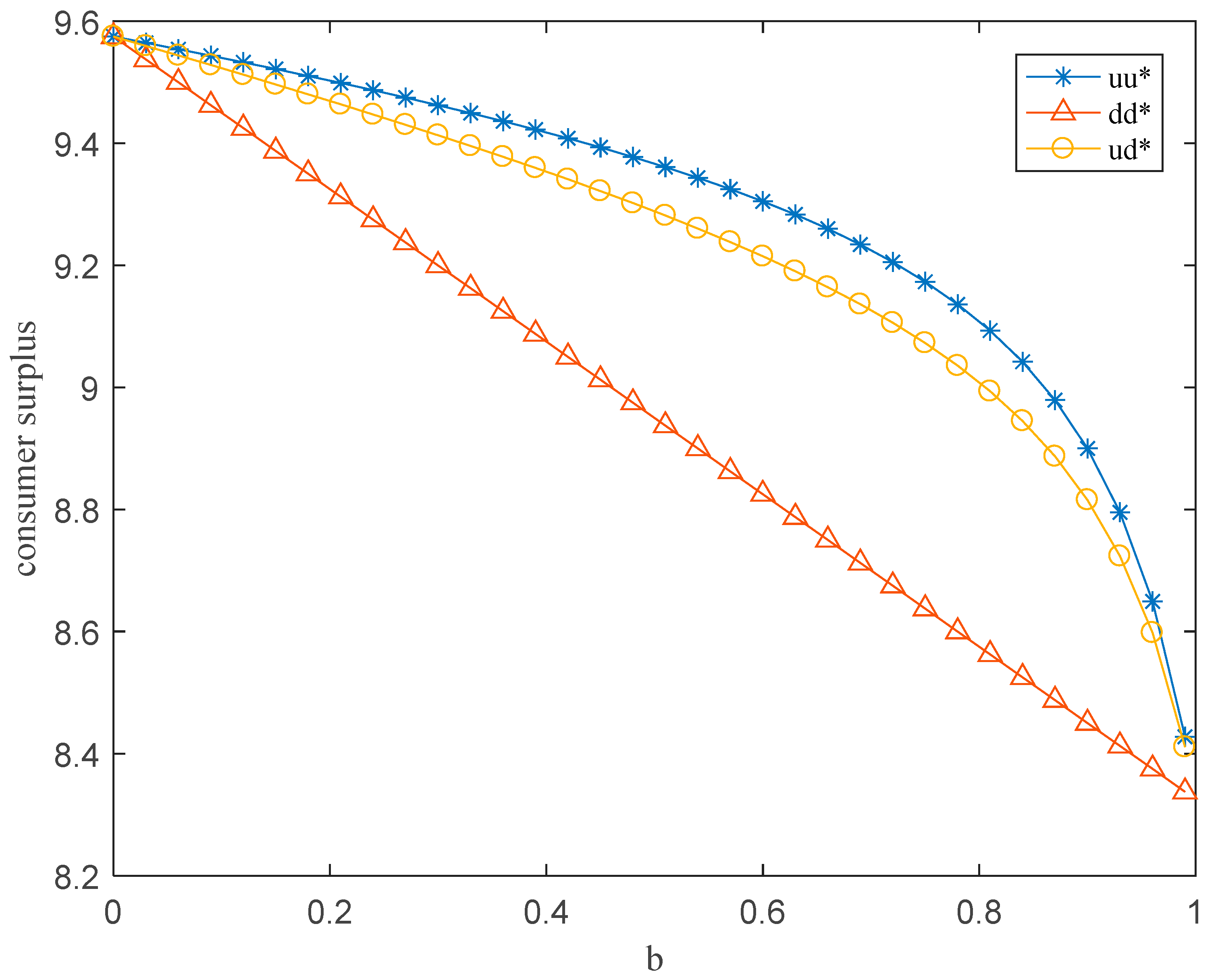
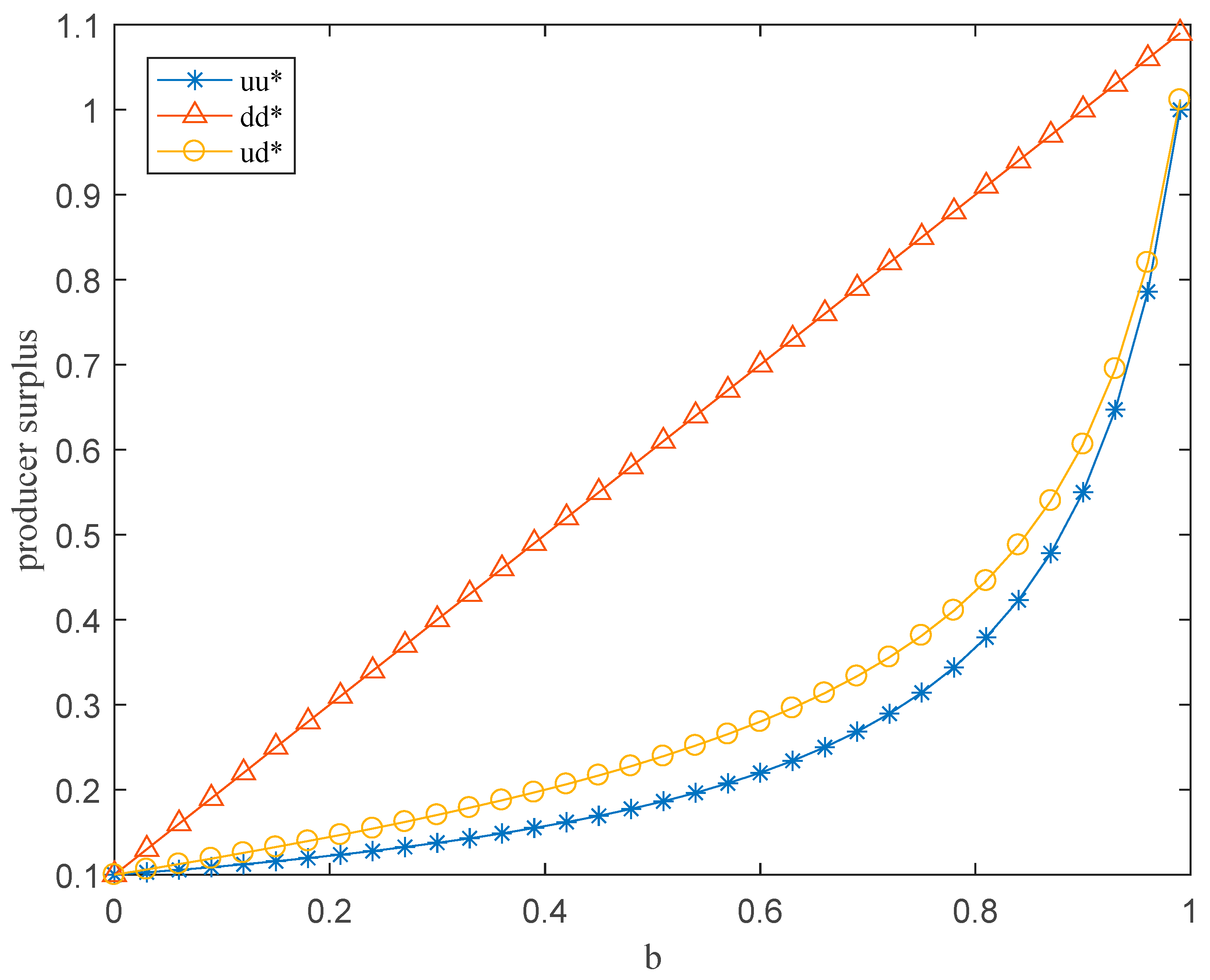
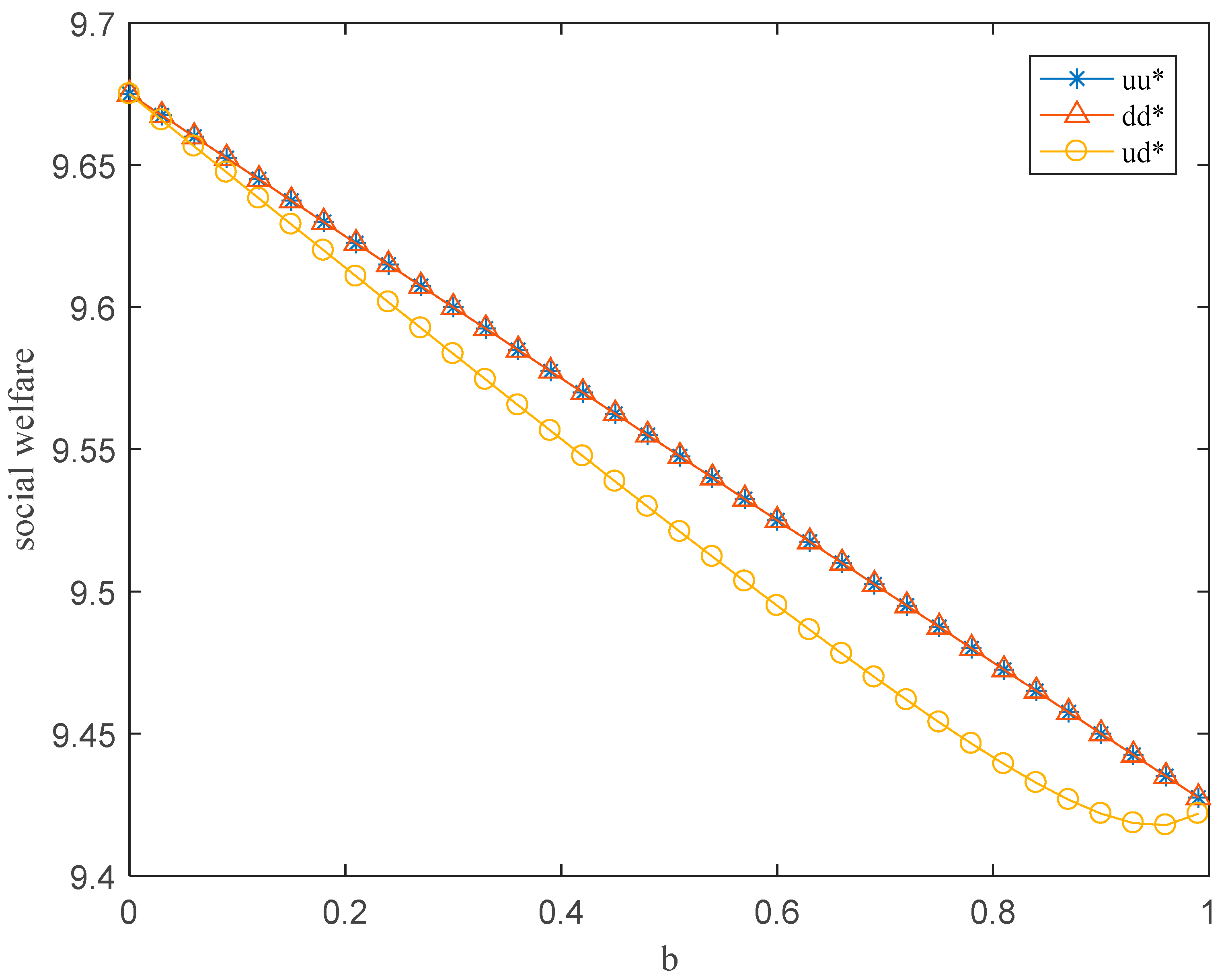
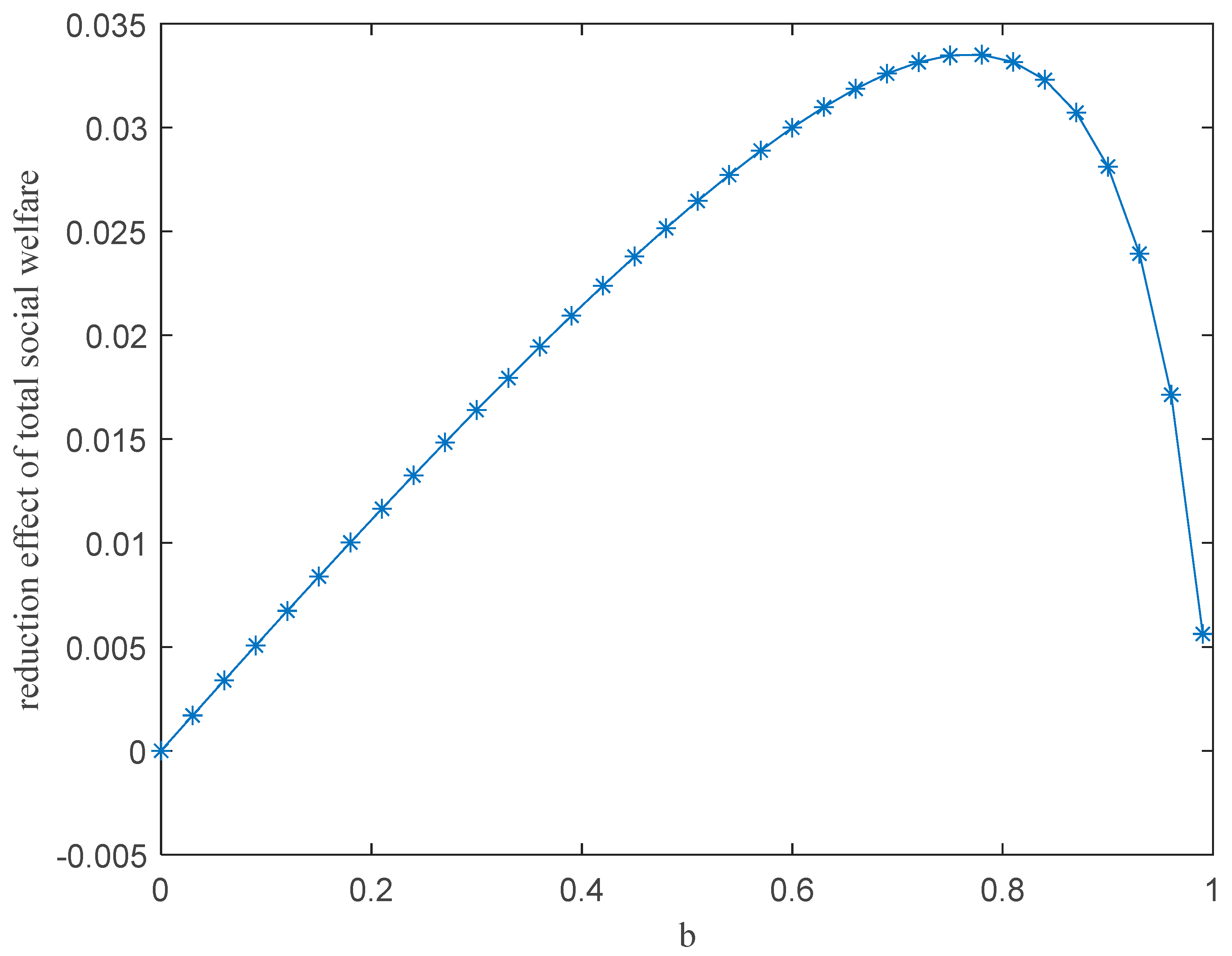
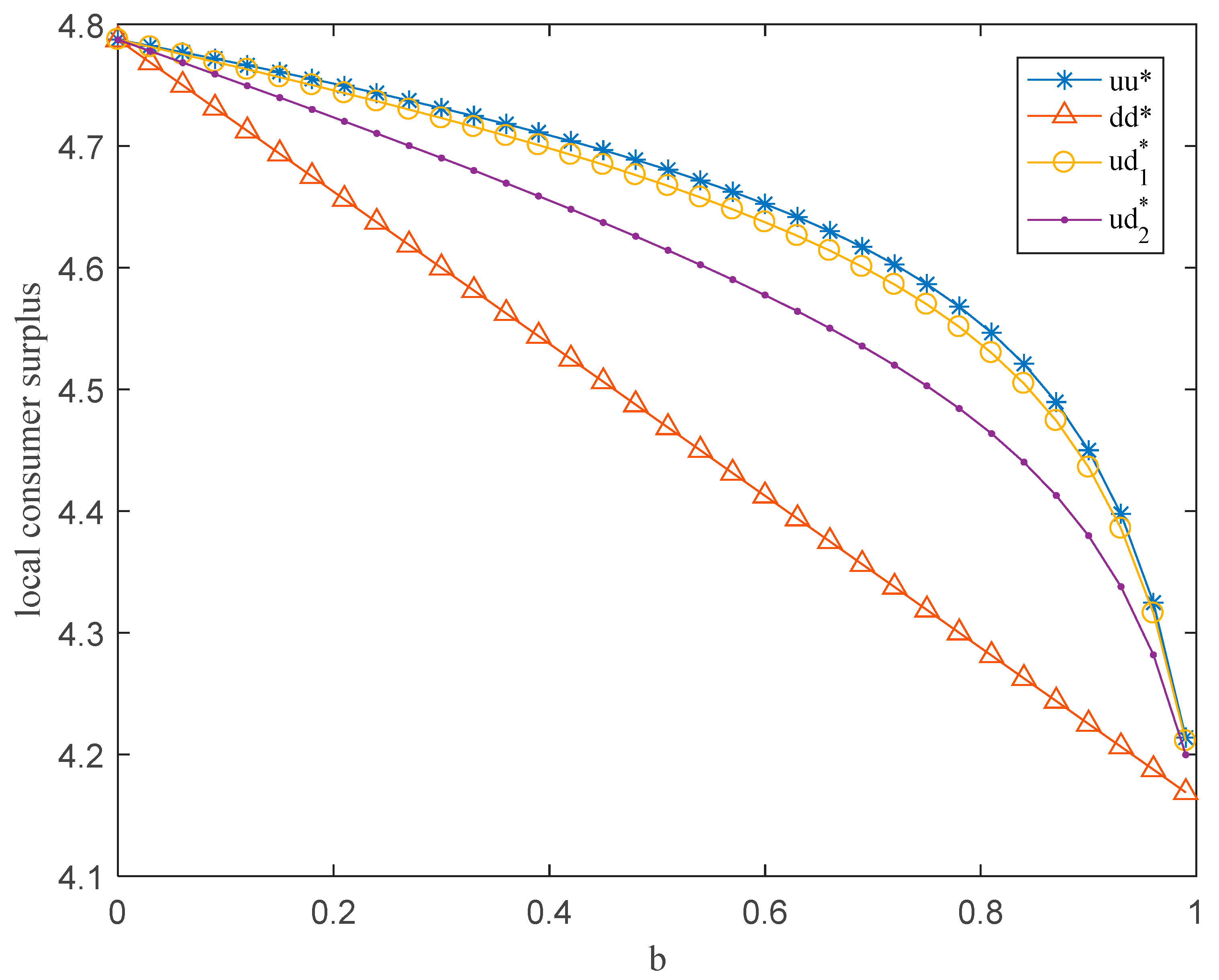
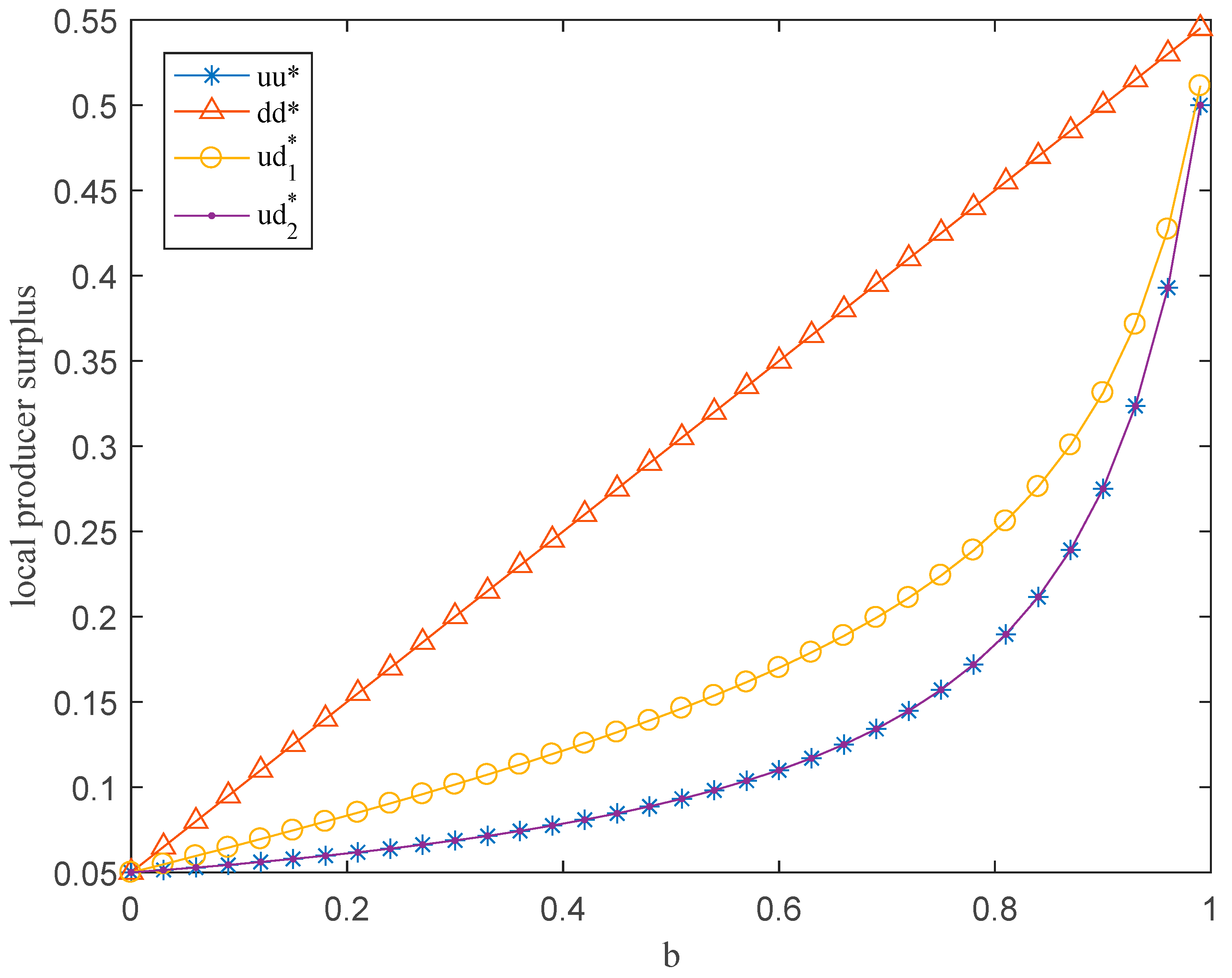
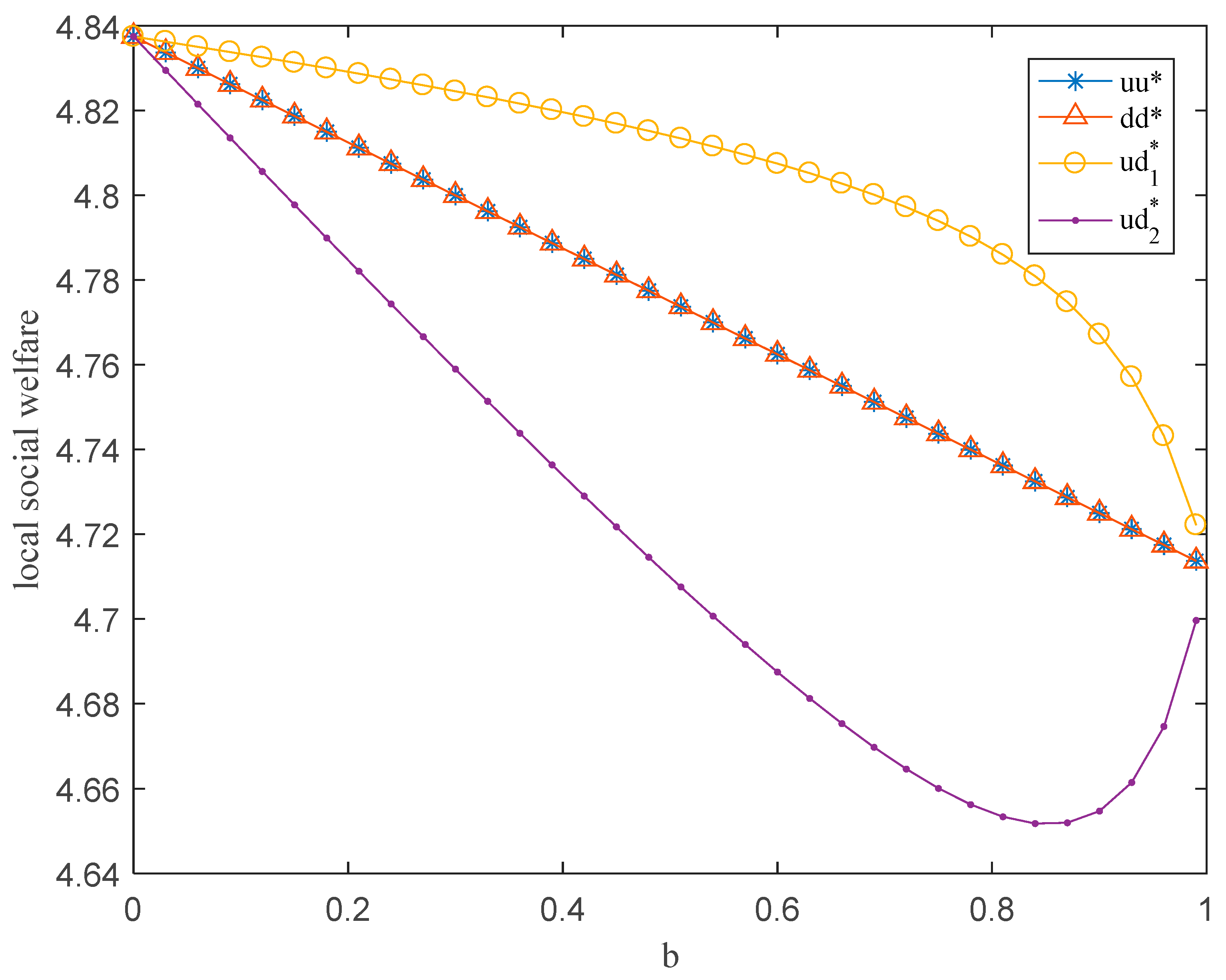
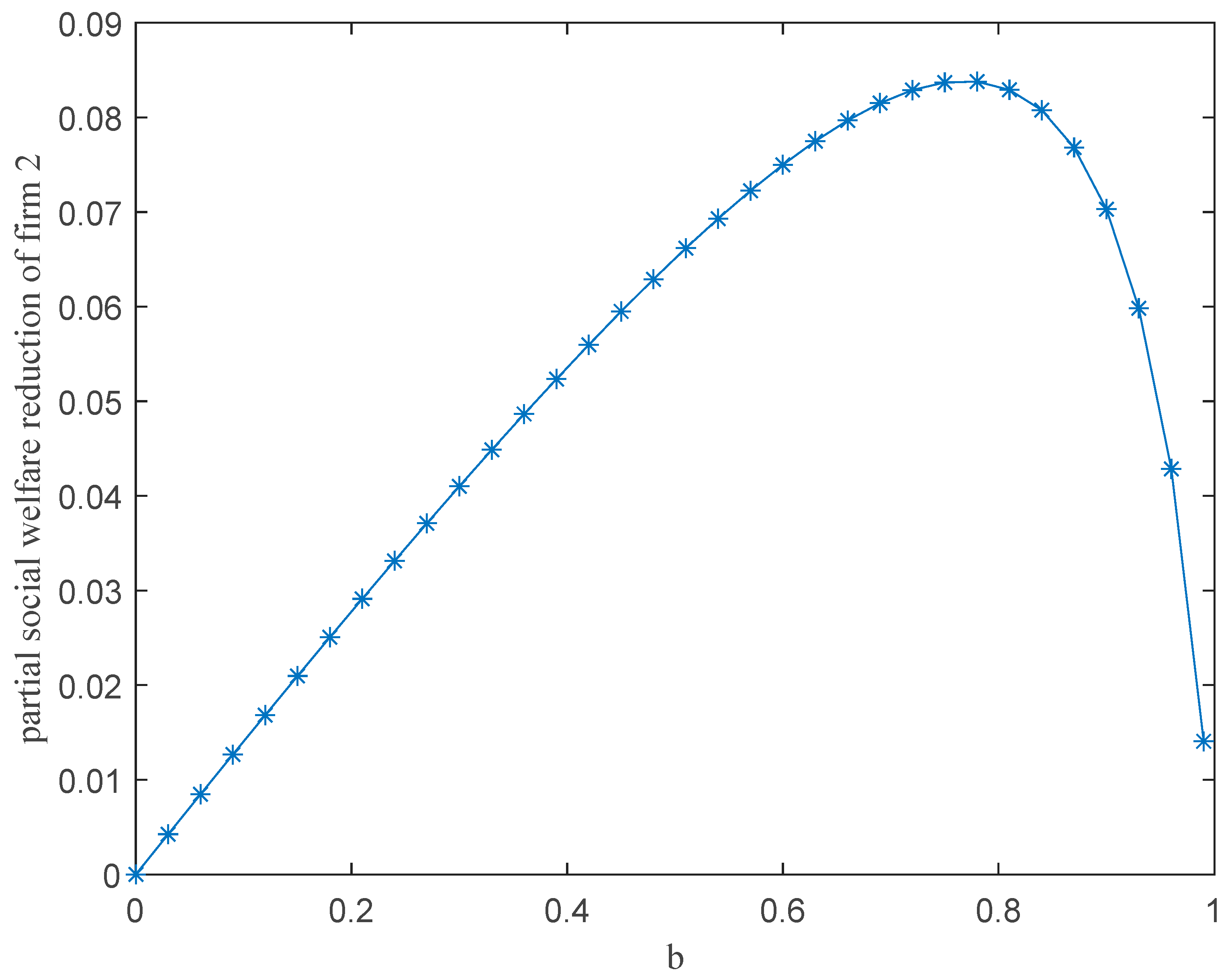
5. Numerical Analysis

In this section, the equilibrium results obtained in different price game situations will be numerically analyzed. The following parameters are set according to our model: V = 10 ,   t A = 1.1 ,   t B = 0.1 ,   c = 0.3 , let b range between 0 and 1.
Firstly, we analyze total consumer surplus, total producer surplus, and total social welfare through MATLAB simulation. Figure 1, Figure 2 and Figure 3 respectively represent the size and change of total consumer surplus, total producer surplus, and total social welfare under different price game situations.
From Figure 1, Figure 2 and Figure 3, we can see that the total consumer surplus is the largest in the “uu” situation, slightly larger in the “ud” situation, and the smallest in the “dd” situation. The size of total producer surplus is opposite to consumer surplus, which is minimum in the “uu” situation, slightly smaller in the “ud” situation, and maximum in the “dd” situation. The total social welfare was the smallest in the “ud” situation and the same in the “uu” situation as in the “dd” situation. It can also be seen that with the increase of the b, the total social welfare first decreased and then increased. This is consistent with the results of Proposition 2 and Lemma 1.
Next, we simulate the reduction effect of the total social welfare, as shown in Figure 4.
It can be seen from Figure 4 that, with the increase of b, the reduction amount of total social welfare increases first and then decreases, which is consistent with the conclusion of Proposition 3.
Then, we conducted a numerical analysis of local social welfare and conducted numerical simulation on local consumer surplus, local producer surplus, and local social welfare with MATLAB. Figure 5, Figure 6 and Figure 7 show the sizes and changes of local consumer surplus, local producer surplus, and local social welfare under different competitive situations.
As can be seen from Figure 5, Figure 6 and Figure 7, the consumer surplus created by firm 1 and firm 2 is the largest in the “uu” situation and the smallest in the “dd” situation; in the “ud” situation, the consumer surplus of firm 1 is also higher than that of firm 2. The profit created by firm 1 and firm 2 is the largest in the “dd” situation and the smallest in the “uu” situation; in the “ud” situation, the profit of firm 1 is higher than that of firm 2. The local social welfare created by firm 1 is the largest in the “ud” situation, but the local social welfare created by firm 2 is the lowest in the “ud” situation. In addition, with the increase of the parameter b, the local social welfare created by firm 1 decreases, but the local social welfare created by firm 2 decreases and then increases. This is consistent with the conclusion of Proposition 4.
Next, we simulate the local social welfare reduction effect of firm 2, as shown in Figure 8.
As can be seen from Figure 8, with the increase of b, the reduction effect of the local social welfare of firm 2 first increases and then decreases, which is consistent with the conclusion of Proposition 5.

6. Conclusions

We investigated the impact of the third-degree price discrimination on welfare under an asymmetric price game between firms in a duopoly market, During the research process, we assumed that there are two groups of consumers in the market, which form two segment markets: strong market and weak market. Under this premise, we built an improved Hotelling model, and some intriguing findings that are different from existing literature can accordingly be summarized as follows: compared with two symmetric price games, in the asymmetric price game, we find that although the total output of each firm remains unchanged, price discrimination vs. uniform pricing leads to misallocation of consumption, which decreases total social welfare. This reduction effect of total social welfare will increase and then decrease with the increase in strong market size.
From the local social welfare analysis, under the asymmetric price game, price discrimination is a dominant strategy for firms; although the output of the firm that uses price discrimination remains unchanged, it has a higher competitive advantage, which profit, consumer surplus, and local social welfare created by its increase significantly. On the contrary, that created by the firm that uses uniform pricing decreases significantly, and with the increase in the strong market size, the reduction effect of social welfare increases first and then decreases.
These findings can be explained by why the government acquiesces price discrimination and also can be explained by why most firms choose price discrimination in oligopoly markets. At the same time, these findings help us recognize the relationship between third-degree price discrimination and social welfare in the asymmetric price game, which guides firms to make price decisions and helps the government to take effective measures and activities to improve social welfare.
Although we have made contributions to the price discrimination and social welfare literature, several directions remain for future research. In this paper, we only considered a fully covered duopoly competitive, which may be slightly different from reality. Therefore, we could expand the competition between two firms to the competition between many firms, and extend the fully covered market to the partially covered market in future research.

Author Contributions

Conceptualization, Z.Z. and Q.M.; methodology, Z.Z.; writing—original draft preparation, Z.Z. and Y.W.; writing—review and editing, Q.H.; supervision, Q.M. and Q.H. All authors have read and agreed to the published version of the manuscript.

Funding

This research was funded by the National Nature Science Foundation of China (NSFC) and grant number 71974115.

Institutional Review Board Statement

Not applicable.

Informed Consent Statement

Not applicable.

Data Availability Statement

Not applicable.

Conflicts of Interest

The authors declare no conflict of interest.

Appendix A

Proof of Lemma 1.
d S W u d d b = 5 ( t A t B ) 16 + t A t B ( t A t B ) 16 [ t B b + t A ( 1 b ) ] 2 , if 5 ( t A t B ) 16 + t A t B ( t A t B ) 16 [ t B b + t A ( 1 b ) ] 2 < 0 ; equivalently, if b t A t A t B / 5 t A t B is satisfied, we can obtain d S W u d d b < 0 ; when b > t A t A t B / 5 t A t B , d S W u d d b > 0 . □
Proof of Proposition 3.
Δ S W = S W u u S W u d = b t A + ( 1 b ) t B 16 t A t B 16 [ t B b + t A ( 1 b ) ] , d Δ S W d b = { [ t B b + t A ( 1 b ) ] 2 t A t B } ( t A t B ) 16 [ t B b + t A ( 1 b ) ] 2 , if [ t B b + t A ( 1 b ) ] 2 t A t B < 0 ; equivalently, if b t A t A t B t A t B is satisfied, we can obtain d Δ S W d b > 0 ; while b > t A t A t B t A t B , d Δ S W d b < 0 . □
Proof of Lemma 2.
d S W 1 u d d b = ( t A t B ) 32 3 t A t B ( t A t B ) 32 [ t B b + t A ( 1 b ) ] 2 < 0 ; while d S W 2 u d d b = [ 9 [ t B b + t A ( 1 b ) ] 2 5 t A t B ] ( t A t B ) 32 [ t B b + t A ( 1 b ) ] 2 , when [ 9 [ t B b + t A ( 1 b ) ] 2 5 t A t B ] ( t A t B ) 32 [ t B b + t A ( 1 b ) ] 2 > 0 ; that is, if b < 3 t A 5 t A t B 3 ( t A t B ) is satisfied, we obtain d S W 2 u d d b < 0 ; while b > 3 t A 5 t A t B 3 ( t A t B ) , d S W 2 u d d b > 0 . □
Proof of Proposition 5.
  Δ S W 2 = S W 2 u u S W 2 u d = 5 [ b t A + ( 1 b ) t B ] 32 5 t A t B 32 [ t B b + t A ( 1 b ) ] ,   d Δ S W 2 d b = 5 { [ t B b + t A ( 1 b ) ] 2 t A t B } ( t A t B ) 32 [ t B b + t A ( 1 b ) ] 2 , if [ t B b + t A ( 1 b ) ] 2 t A t B < 0 ; equivalently, if b t A t A t B t A t B is satisfied, we obtain d Δ S W 2 d b > 0 , while b > t A t A t B t A t B , d Δ S W 2 d b < 0 . □

References

  1. Varian, H.R. Price Discrimination and Social Welfare. Am. Econ. Rev. 1985, 75, 870–875. [Google Scholar]
  2. Askar, S.; Foul, A.; Mahrous, T.; Djemele, S.; Ibrahim, E. Global and Local Analysis for a Cournot Duopoly Game with Two Different Objective Functions. Mathematics 2021, 9, 3119. [Google Scholar] [CrossRef]
  3. Robinson, J. The Economics of Imperfect Competition; Springer Macmillan: London, UK, 1993. [Google Scholar]
  4. Clempner, J.B.; Poznyak, A.S. Analytical Method for Mechanism Design in Partially Observable Markov Games. Mathematics 2021, 9, 321. [Google Scholar] [CrossRef]
  5. Schmalensee, R. Output and Welfare Implications of Monopolistic Third-degree Price Discrimination. Am. Econ. Rev. 1981, 71, 242–247. [Google Scholar]
  6. Namin, A.; Gauri, D.K.; Kwortnik, R.J. Improving Revenue Performance with Third-degree Price Discrimination in the Cruise Industry. Int. J. Hosp. Manag. 2020, 89, 102597. [Google Scholar] [CrossRef]
  7. Schwartz, M. Third-degree price discrimination and output: Generalizing welfare result. Am. Econ. Rev. 1990, 80, 1259–1262. [Google Scholar]
  8. Adams, C.F. A Note on Pricing with Market Power: Third-degree Price Discrimination with Quality-differentiated Demand. Am. Econ. 2019, 64, 183–187. [Google Scholar] [CrossRef]
  9. Wang, X.; Zhang, L. Monopolistic third-degree price discrimination, welfare, and vertical market structure. Rev. Econ. Des. 2021, 26, 75–86. [Google Scholar] [CrossRef]
  10. Holmes, T.J. The effects of third-degree price discrimination in oligopoly. Am. Econ. Rev. 1989, 79, 244–250. [Google Scholar]
  11. Corts, K.S. Third-degree Price Discrimination in Oligopoly: All-out Competition and Strategic Commitment. RAND J. Econ. 1998, 29, 306–323. [Google Scholar] [CrossRef]
  12. Miklós-Thal, J.; Shaffer, G. Third-degree price discrimination in oligopoly with endogenous input costs. Int. J. Ind. Organ. 2021, 79, 102713. [Google Scholar] [CrossRef]
  13. Aguirre, I. Oligopoly Price Discrimination, Competitive Pressure and Total Output. Economics 2019, 13, 1–16. [Google Scholar] [CrossRef] [Green Version]
  14. Armstrong, M.; Vickers, J. Competitive price discrimination. RAND J. Econ. 2001, 32, 579–605. [Google Scholar] [CrossRef]
  15. Chen, Y.; Schwartz, M. Beyond price discrimination: Welfare under differential pricing when costs also differ. MPRA Pap. 2012, 11, 1–29. [Google Scholar]
  16. Adachi, T.; Matsushima, N. The welfare effects of –third-degree price discrimination in a differentiated oligopoly. Econ. Inq. 2014, 52, 1231–1244. [Google Scholar] [CrossRef] [Green Version]
  17. Galera, F.; Mendi, P.; Molero, J.C. Quality differences, third-degree price discrimination, and welfare. Econ. Inq. 2017, 55, 339–351. [Google Scholar] [CrossRef] [Green Version]
  18. Feng, H.; Ma, J. Location choices and third-degree spatial price discrimination. Scot. J. Polit. Econ. 2018, 2, 142–153. [Google Scholar] [CrossRef]
  19. Zhang, T.; Huo, Y.; Zhang, X.; Shuai, J. Endogenous third-degree price discrimination in Hotelling model with elastic demand. J. Econ. 2019, 127, 125–145. [Google Scholar] [CrossRef]
  20. Galera, F.; Garcia-del-Barrio, P.; Mendi, P. Consumer surplus bias and the welfare effects of price discrimination. J. Regul. Econ. 2019, 55, 33–45. [Google Scholar] [CrossRef]
  21. Chung, H.S. Welfare impacts of behavior-based price discrimination with asymmetric firms. Asia-Pac. J. Bus. Adm. 2020, 11, 17–26. [Google Scholar] [CrossRef]
  22. Yl, A.; Jie, S.B. Monopolistic competition, price discrimination, and welfare. Econ. Lett. 2019, 174, 114–117. [Google Scholar]
Figure 1. The total consumer surplus under different situations.
Mathematics 10 01215 g001
Figure 2. The total producer surplus under different situations.
Mathematics 10 01215 g002
Figure 3. The total social welfare under different situations.
Mathematics 10 01215 g003
Figure 4. The reduction effect of the total social welfare.
Mathematics 10 01215 g004
Figure 5. The local consumer surplus under different situations.
Mathematics 10 01215 g005
Figure 6. The local producer surplus under different situations.
Mathematics 10 01215 g006
Figure 7. The local social welfare under different situations.
Mathematics 10 01215 g007
Figure 8. The reduction effect of the local social welfare of firm 2.
Mathematics 10 01215 g008
Publisher’s Note: MDPI stays neutral with regard to jurisdictional claims in published maps and institutional affiliations.

