3D Flow of Hybrid Nanomaterial through a Circular Cylinder: Saddle and Nodal Point Aspects

Abstract

This mathematical model explains the behavior of sinusoidal radius activity in stagnation point three-dimensional flow of hybrid nanoparticles through a circular cylinder. The energy equation of heat source/sink effect and the mass equation of Arrhenius energy of activation and chemical reaction effects are incorporated. Self-relation transformations are adopted to reduce the PDEs to ODEs, then the RKF-45 method is solved with shooting proficiency. The nodal and saddle point action is studied in pertinent parameters for thermal, mass, and velocity curves. Further statistical values of skin friction, Nusselt number, and Sherwood number of both nodal and saddle points are portrayed in tables format. It is ascertained that higher values of activation energy and reaction rate enhance the concentration curve. In addition, the nodal point curves are always less than saddle point curves.

1. Introduction

Nanofluids are very fine engineering colloidal particles created by combining nanoparticles and a base liquid. The diameter of nanoparticles typically ranges from 1–100 nm, and the base liquid is typically water or ethyl glycerol. Choi [1] in 1995 was the first to suggest the effects of thermal conductivity and heat transmission across nanofluids. In addition, based on his assessment, he discovered that nanofluids are more efficient than base fluids. Because the nanofluid is one of the developing liquids, it has resulted in numerous scientific inventions in the nano industries, according to Choi’s survey [2]. Many of academics have examined a range of analyses of fluid models across various platforms (see refs. [3,4,5,6,7,8,9]). Hybrid nanofluids have recently taken precedence over nanofluids due to increased thermal conductivity and a more efficient heat transference rate. Hybrid nanofluids are created by combining two or more nanoparticles with a base liquid. The various applications of hybrid nanofluids were studied by Sarkar et al. [10]. Stability and various characteristics of CuO–TiO₂/water-based hybrid nanofluid were examined by Asadi et al. [11]. Lund et al. [12] studied the dual solution of the impact of thermal radiation effect over magnetohydrodynamic flow of a Cu–Al₂O₃/H₂O-based hybrid nanofluid. Ramesh et al. [13] investigated the Darcy–Forchheimer model of hybrid nanofluid in a stretchable convergent/divergent channel. They found variations of velocity and solid volume fraction in the channel. Ramesh and Madhukesh [14] investigated the effect of hybrid carbon nanotubes in the presence of activation energy and heat source/sink. They found that hybrid CNTs nanomaterials have a greater rate of heating/cooling than single CNTs nanomaterials.

Many aspects, such as activation energy, heat source/sink, and slip parameters, all play a significant part in thermal and concentration analyses of fluid flow. These variables enable us to examine the behavior of fluids over a range of parameters. Alghamdi et al. [15] studied the role of dyadic chemical response for the MHD flow of viscous fluid with suspended nanoparticles through the gyrating disk. Rekha et al. [16] considered AA7072-AA7075/water-based hybrid nanofluid flowing through a cone, wedge, and plate in the presence of activation energy. They discussed the impact of activation energy and mass transfer phenomena in the presence of hybrid nanofluid. Ramesh [17] used Buongiorno’s model to analyze the significance of chemical reaction and energy of activation over a viscoelastic nanomaterial through a surface with stretching. Further, this model was taken and work was extended by Alsadi et al. [18], who, over stretching sheet, studied the entropy generation impact, and Asma et al. [19], who examined the influence of Arrhenius energy of activation on Darcy–Forchheimer nano liquid in three dimension.

A three-dimensional Williamson nanofluid with Darcy–Forchheimer permeable media was emphatically deliberated upon by Ramzan et al. [20]. They found the behavior of heat flux under the Fourier and Fick’s laws and examined the Williamson and Hartman number over a velocity profile. Jagan et al. [21] deliberated the 3D unsteady MHD convective stream of nano liquid with double stratification using the homotopy analysis method. Nayak et al. [22] explored the three-dimensional free convective moment of a radioactive nanofluid under a variable magnetic field. They observed the influence of the Hartmann number on the temperature and thickness of the related boundary layer. Irfan et al. [23] scrutinized the nonlinear mixed convection on radioactive flow and activation energy on the 3D flow of a Carreau nanofluid. Alwawi et al. [24] investigated the ethyl-glycerol-based nanofluid flow around a circular cylinder by utilizing the Tiwari and Das [25] nanofluid model. In this study, they considered the magnetohydrodynamic effect and analyzed the heat transfer effects.

Inspired by all the above insights, we developed a 3D flow of hybrid nanoparticles (${\mathrm{Fe}}_3{\mathrm{O}}_4+\mathrm{Go}$) through a circular cylinder in the stagnation point region. From the literature point of view, the problem has not yet been studied by considering activation energy. Normal partial coupled equations are regenerated ordinary coupled equations. Furthermore, equations are solved numerically with the prominent RKF-45 method. A good discussion is made with the help of graphs.

2. Problem Formulation

Consider a time-independent, three-dimensional flow of a hybrid nanofluid (${\mathrm{Fe}}_3{\mathrm{O}}_4+\mathrm{Go}$) with water as a base fluid in the direction of the circular cylinder (see Figure 1). The radius of the cylinder variegates sinusoidally. The positions B, A, and C on the cylinder represent the minimum and maximum stagnation points. A connecting line connects A to B and B to C, splitting the flow that passes on either side of the cylinder. Additionally, the flow is taken with $u_e^{*}\&v_e^{*}$ free stream speed along the $x\&y$ direction, with $c=\frac{b^{*}}{a^{*}}$ representing the special streamline. The flow lines of the nodal stagnation point are ranging from $0<c<1$, The flow lines of the saddle stagnation point are ranging from $-1<c<0$. The flow is said to plane when $c=0$. The Arrhenius energy of activation, chemical reaction, and uniform heat source/sink effects are examined. The equations which represent the above-assumed flow are given as follows (see [26,27]).

Continuity equation

$$\frac{\partial u}{\partial x}+\frac{\partial v}{\partial y}+\frac{\partial w}{\partial z}=0$$

(1)

Momentum equation

$$u\frac{\partial u}{\partial x}+v\frac{\partial u}{\partial y}+w\frac{\partial u}{\partial z}=a^{*2}x+{\nu }_{hnf}\frac{{\partial }^{2}u}{\partial z^2}$$

(2)

$$u\frac{\partial v}{\partial x}+v\frac{\partial v}{\partial y}+w\frac{\partial v}{\partial z}=b^{*2}y+{\nu }_{hnf}\frac{{\partial }^{2}v}{\partial z^2}$$

(3)

Temperature equation

$$u\frac{\partial T}{\partial x}+v\frac{\partial T}{\partial y}+w\frac{\partial T}{\partial z}={\alpha }_{hnf}\frac{{\partial }^{2}T}{\partial z^2}+\frac{Q_0}{{(\rho c_p)}_{hnf}}(T-T_{\infty })$$

(4)

Concentration equation

$$u\frac{\partial C}{\partial x}+v\frac{\partial C}{\partial y}+w\frac{\partial C}{\partial z}=D_{hnf}\frac{{\partial }^{2}C}{\partial z^2}-{\kappa }_r^2{\left(\frac{T}{T_{\infty }}\right)}^n{e}^{-\frac{E_a}{KT}}(C-C_{\infty })$$

(5)

The interrelated boundary constraints are

$$u=0,\hspace{1em}v=0,\hspace{1em}w=0,\hspace{1em}\gamma k_{hnf}\frac{\partial T}{\partial z}=T-T_w,\hspace{1em}C=C_w\hspace{1em}at\hspace{1em}z=0,$$

(6)

$$u\to u_e^{*},\hspace{1em}v\to v_e^{*},\hspace{1em}T\to T_{\infty },\hspace{1em}C\to C_{\infty } as\hspace{1em}z\to \infty$$

(7)

where ($u, v, w \mathrm{and} T$) are the components of velocity and temperature along x, y, and z directions. $a^{*2}$ and $b^{*2}$ represent the free stream-dependent constants. The term $\nu \left(=\frac{\mu }{\rho }\right)$ denotes kinematic viscosity, and $\mu$ and $\rho$ represent dynamic viscosity and density of the hybrid nanofluid, respectively. $\alpha \left(=\frac{k}{\left(\rho C_p\right)}\right)$ denotes hybrid nanofluid’s thermal diffusivity, and the term $k$ represents thermal conductivity. $T_w\&C_w$ represent the temperature and concentration at the wall, and $T_{\infty }\&C_{\infty }$ represent ambient temperature and concentration. $Q_0$ is the uniform heat source/sink coefficient, ${\kappa }_r^2$ is the reaction rate, $n$ denotes the fitted rate constant, $K$ is the Boltzmann constant, $E_a$ is activation energy, and ${\left(\frac{T}{T_{\infty }}\right)}^n{e}^{-\frac{E_a}{KT}}$ is modified Arrhenius function. $\gamma$ is thermal slip, and the subscript $hnf$ denotes hybrid nanofluid. Thermophysical features of water and nanoparticles are listed in

Table 1. Thermophysical properties of nanoparticles and water.

Particles	$\mathit{\rho }(\mathbf{k}\mathbf{g}/{\mathbf{m}}^3)$	${\mathit{c}}_{\mathit{p}}(\mathbf{J}/\mathbf{k}\mathbf{g} \mathbf{K})$	$\mathit{k}(\mathbf{W}/\mathbf{m}\mathbf{K})$
${\mathrm{Fe}}_3{\mathrm{O}}_4$	5180	670	9.7
$\mathrm{Go}$	1800	717	5000
Water	997.1	4179	0.613

(see [28]).

The efficient characteristics of hybrid nanofluid are stated below.

$$\begin{array}{l}{D}_{hnf}={(1-{\varphi }_1)}^{2.5}{(1-{\varphi }_2)}^{2.5}{D}_f,\\ {\left(\rho C_p\right)}_{hnf}={(1-{\varphi }_1)}^{2.5}{(1-{\varphi }_2)}^{2.5}{\left(\rho C_p\right)}_f+{\varphi }_1{\left(\rho C_p\right)}_{S1}+{\varphi }_2{\left(\rho C_p\right)}_{S2},\\ {\mu }_{hnf}=\frac{{\mu }_f}{{(1-{\varphi }_1)}^{2.5}{(1-{\varphi }_2)}^{2.5}},{\rho }_{hnf}=\left(1-{\varphi }_2\right)\left[(1-{\varphi }_1){\rho }_f+{\varphi }_1{\rho }_{s1}\right]+{\varphi }_2{\rho }_{\begin{array}{l}s2\end{array}},\\ {\left(\rho c_p\right)}_{hnf}=\left(1-{\varphi }_2\right)\left[(1-{\varphi }_1){\left(\rho c_p\right)}_f+{\varphi }_1{\left(\rho c_p\right)}_{s1}\right]+{\varphi }_2{\left(\rho c_p\right)}_{s2},\\ k_{hnf}=\frac{k_{s_2}+(m_1-1)k_{bf}-(m_1-1){\varphi }_2(k_{bf}-k_{s_2})}{k_{s_2}+(m_1-1)k_{bf}+{\varphi }_2(k_{bf}-k_{s_2})}{k}_{bf},\\ \mathrm{where} k_{bf}=\frac{k_{s_1}+(m_1-1)k_f-(m_1-1){\varphi }_1(k_f-k_{s_1})}{k_{s_1}+(m_1-1)k_f+{\varphi }_1(k_f-k_{s_1})}{k}_f\end{array}\}$$

(8)

Here, ${\varphi }_1,\hspace{1em}{\varphi }_2$ indicates the volume fraction of individual nanoparticles. Here, suffixes $hnf$ denote hybrid nanofluid, $f$ denote base fluid, and $s$ denote solid particle, and $m_1$ is shape factor parameter. In the current study, we take a sphere shape $\left(m_1=3\right)$ [29].

The variables are used to obtain the similarity equations:

$$\begin{array}{l}u=a^{*}{xf}^{\prime }(\eta ),\hspace{1em}v=b^{*}{yg}^{\prime }(\eta ),\hspace{1em}w=-\sqrt{a^{*}{\nu }_f}\left(f(\eta )+cg(\eta )\right),\\ T=T_{\infty }+(T_w-T_{\infty })\theta (\eta ),\hspace{1em}C=C_{\infty }+(C_w-C_{\infty })\chi (\eta ),\hspace{1em}\eta =z\sqrt{\frac{a^{*}}{{\nu }_f}}.\end{array}\}$$

(9)

The transformed ordinary differential equations along with the conditions are

$$\begin{array}{l}\frac{1}{{(1-{\varphi }_1)}^{2.5}{(1-{\varphi }_2)}^{2.5}\left[\left\{(1-{\varphi }_2)(1-{\varphi }_1)+{\varphi }_1\frac{{\rho }_{s_1}}{{\rho }_f}\right\}+{\varphi }_2\frac{{\rho }_{s_2}}{{\rho }_f}\right]}{f}^{‴}\\ +f{f}^{″}+c{f}^{″}g-f^{{}^{\prime }2}+1=0\end{array}$$

(10)

$$\begin{array}{l}\frac{1}{{(1-{\varphi }_1)}^{2.5}{(1-{\varphi }_2)}^{2.5}\left[\left\{(1-{\varphi }_2)(1-{\varphi }_1)+{\varphi }_1\frac{{\rho }_{s_1}}{{\rho }_f}\right\}+{\varphi }_2\frac{{\rho }_{s_2}}{{\rho }_f}\right]}{g}^{‴}\\ +f{g}^{″}+c{g}^{″}g-c{g}^{{}^{\prime }2}+c=0\end{array}$$

(11)

$$\frac{\frac{k_{hnf}}{k_f}}{\mathrm{Pr}\left[\left\{(1-{\varphi }_2)(1-{\varphi }_1)+{\varphi }_1\frac{{(\rho c_p)}_{s_1}}{{(\rho c_p)}_f}\right\}+{\varphi }_2\frac{{(\rho c_p)}_{s_2}}{{(\rho c_p)}_f}\right]}{\theta }^{″}+f{\theta }^{\prime }+c{\theta }^{\prime }g+S\theta =0$$

(12)

$${(1-{\varphi }_1)}^{2.5}{(1-{\varphi }_2)}^{2.5}{\chi }^{″}+Scf{\chi }^{\prime }+c Sc{\chi }^{\prime }g-\beta Sc{(1+\delta \theta )}^{n}Exp\left(\frac{-E}{1+\delta \theta }\right)\chi =0$$

(13)

The reduced boundary constraints are

$$\begin{array}{l}{f}^{\prime }(0)=0,\hspace{1em}{g}^{\prime }(0)=0,\hspace{1em}f(0)=0,\hspace{1em}\\ g(0)=0,\hspace{1em}\theta (0)=1+\lambda \frac{k_{hnf}}{k_f}{\theta }^{\prime }(0), \chi (0)=1\end{array}\} \mathrm{at} \eta \to 0$$

(14)

$$f^{\prime }(\infty )\to 1,\hspace{1em}{g}^{\prime }(\infty )\to 1,\hspace{1em}\theta (\infty )\to 0, \chi (\infty )\to 0 \mathrm{as} \eta \to \infty$$

(15)

The variables which are present in the Equations (9)–(13) are as follows:

$c=\frac{b^{*}}{a^{*}}$ is a constant that represents a streamline, $\lambda =\gamma k_f\sqrt{\frac{a^{*}}{{\nu }_f}}$ is the thermal slip parameter, $\mathrm{Pr}=\frac{{\mu }_f{(C_p)}_f}{k_f}$ is a Prandtl number, $Sc=\frac{{\nu }_f}{D_f}$ is a Schmidt number, $E=\frac{E_a}{K{T}_{\infty }}$ is the activation energy, $\delta =\frac{T_w-T_{\infty }}{T_{\infty }}$ is temperature difference parameter, $\beta =\frac{{\kappa }_r^2}{a^{*}}$ is reaction rate, and $S=\frac{Q_0}{a^{*}{(\rho Cp)}_{hnf}}$ is the heat source/sink parameter.

Skin friction, Nusselt, and Sherwood numbers are given by

$$C_{fx}=\frac{{\tau }_{wx}}{{\rho }_f{u}_w^2},\hspace{1em}{C}_{fy}=\frac{{\tau }_{wy}}{{\rho }_f{u}_w^2},\hspace{1em}N{u}_x=\frac{x{q}_w}{k_f(T_w-T_{\infty })},\hspace{1em}S{h}_x=\frac{D_{f}x{j}_w}{(C_w-C_{\infty })}$$

(16)

where ${\tau }_{wx}$ and ${\tau }_{wy}$ are the shear stresses surface in the x and y directions.

The surface heat flux is denoted as $q_w$ and mass transfer $j_w$ is defined as

$${\tau }_{wx}={\left[{\mu }_{hnf}\frac{\partial u}{\partial z}\right]}_{z=0}, {\tau }_{wy}={\left[{\mu }_{hnf}\frac{\partial v}{\partial z}\right]}_{z=0}, q_w=-k_{hnf}{\left(\frac{\partial T}{\partial z}\right)}_{z=0}, j_w=-\frac{1}{D_{hnf}}{\left(\frac{\partial C}{\partial z}\right)}_{z=0}$$

(17)

From the above equations, the skin friction, Sherwood, and Nusselt numbers are

$$\begin{array}{l}\sqrt{{\mathrm{Re}}_x}{C}_{fx}=\frac{f^{″}(0)}{{(1-{\varphi }_1)}^{2.5}{(1-{\varphi }_2)}^{2.5}},\hspace{1em}(x/y)\sqrt{{\mathrm{Re}}_x}{C}_{fy}=\frac{c{g}^{″}(0)}{{(1-{\varphi }_1)}^{2.5}{(1-{\varphi }_2)}^{2.5}},\hspace{1em}\\ \frac{N{u}_x}{\sqrt{{\mathrm{Re}}_x}}=-\frac{k_{hnf}}{k_f}{\theta }^{\prime }(0), \frac{S{h}_x}{\sqrt{{\mathrm{Re}}_x}}=-\frac{{\chi }^{\prime }(0)}{{(1-{\varphi }_1)}^{2.5}{(1-{\varphi }_2)}^{2.5}} .\end{array}$$

(18)

where $\mathrm{Re}=\frac{x^2{a}^{*}}{{\nu }_f}$ is Reynolds number.

3. Numerical Procedure and Validation of Code

The reduced equations as stated in (10)–(13) and boundary conditions (14) and (15) are numerically tackled with the help of a well-known numerical approach i.e., Runge–Kutta–Fehlberg-45 order. To obtain the numerical solution, the following steps are followed.

• Convert the BVP into IVP of the first order.
• Apply the shooting procedure to guess the missing boundary values.
• Apply the RKF-45 method to obtain the solution to IVP.
• Find the residuals for all the boundary conditions.
• If the residual error is greater than the error tolerance, adjust the initial guesses.
• If the residual error is less than error tolerance, numerical results are obtained.

Let us consider

$$\begin{array}{l}{\Delta }_1={(1-{\varphi }_1)}^{2.5}{(1-{\varphi }_2)}^{2.5},\\ {\Delta }_2=\left\{(1-{\varphi }_2)(1-{\varphi }_1)+{\varphi }_1\frac{{\rho }_{s_1}}{{\rho }_f}\right\}+{\varphi }_2\frac{{\rho }_{s_2}}{{\rho }_f},\\ {\Delta }_3=\left\{(1-{\varphi }_2)(1-{\varphi }_1)+{\varphi }_1\frac{{(\rho c_p)}_{s_1}}{{(\rho c_p)}_f}\right\}+{\varphi }_2\frac{{(\rho c_p)}_{s_2}}{{(\rho c_p)}_f},\\ f={\vartheta }_1,f^{\prime }={\vartheta }_2,f^{″}={\vartheta }_3\\ g={\vartheta }_4,g^{\prime }={\vartheta }_5,g^{″}={\vartheta }_6\\ \theta ={\vartheta }_7,{\theta }^{\prime }={\vartheta }_8\\ \chi ={\vartheta }_9,{\chi }^{\prime }={\vartheta }_{10}\end{array}$$

$${{\vartheta }_3}^{\prime }=-{\Delta }_1{\Delta }_2\left({\vartheta }_1{\vartheta }_3+c{\vartheta }_3{\vartheta }_4-{\vartheta }_2{}^2+1\right)$$

(19)

$${{\vartheta }_6}^{\prime }=-{\Delta }_1{\Delta }_2({\vartheta }_1{\vartheta }_6+c{\vartheta }_6{\vartheta }_4-c{\vartheta }_5{}^2+c)$$

(20)

$${{\vartheta }_8}^{\prime }=-\mathrm{Pr}{\Delta }_3{k}_f\left({\vartheta }_1{\vartheta }_8+c{\vartheta }_8{\vartheta }_4+S{\vartheta }_7\right)/k_{hnf}$$

(21)

$${{\vartheta }_{10}}^{\prime }=-\left(Sc{\vartheta }_1{\vartheta }_{10}+c Sc{\vartheta }_{10}{\vartheta }_4-\beta Sc{(1+\delta {\vartheta }_7)}^{n}Exp\left(\frac{-E}{1+\delta {\vartheta }_7}\right){\vartheta }_9\right)/{\Delta }_1$$

(22)

and

$$\begin{array}{l}{\vartheta }_2(0)=0,\hspace{1em}{\vartheta }_5(0)=0,\hspace{1em}{\vartheta }_1(0)=0,\\ {\vartheta }_4(0)=0,\hspace{1em}{\vartheta }_7(0)=1+\lambda \frac{k_{hnf}}{k_f}{\vartheta }_8(0), {\vartheta }_9(0)=1\\ \& {\vartheta }_3(0)={\xi }_1,{\vartheta }_6(0)={\xi }_2,{\vartheta }_{10}(0)={\xi }_3\end{array}\}$$

(23)

The algorithm for the numerical procedure (Figure 2) and RKF-45 scheme ([30,31,32]) is given as follows.

In the RKF-45 method, each step uses the following values:

$$\begin{array}{l}{s}_1=f\left(x_i,y_i\right)h_1\\ s_2=f\left(x_i+\frac{1}{4}h,y_i+\frac{1}{4}{s}_1\right)h_1\\ s_3=f\left(x_i+\frac{3}{8}h,y_i+\frac{3}{32}{s}_1+\frac{9}{32}{s}_2\right)h_1\\ s_4=f\left(x_i+\frac{12}{13}h,y_i+\frac{1932}{2147}{s}_1-\frac{7200}{2147}{s}_2+\frac{7296}{2147}{s}_3\right)h_1\\ s_5=f\left(x_i+h,y_i+\frac{439}{216}{s}_1-\frac{845}{4104}{s}_4-8s_2+\frac{3680}{513}{s}_3\right)h_1\\ s_6=f\left(x_i+\frac{1}{2}h,y_i-\frac{8}{27}{s}_1+2s_2-\frac{11}{40}{s}_5-\frac{3544}{2565}{s}_3-\frac{1859}{4104}{s}_4\right)h_1\end{array}$$

Then, using a Runge–Kutta technique of order 4, an estimate of the I.V.P. result is generated.

$$y_{i+1}=y_i+\frac{25}{216}{s}_1-\frac{1}{5}{s}_5+\frac{2197}{4104}{s}_4+\frac{1408}{2565}{s}_3$$

The Runge–Kutta technique of order 5 is given by

$$z_{i+1}=y_i+\frac{16}{135}{s}_1+\frac{2}{55}{s}_6-\frac{9}{50}{s}_5+\frac{28561}{56430}{s}_4+\frac{6656}{12825}{s}_3$$

The numerical results are validated with available previously published works (see Gangadar et al. [33], Bhattacharyya and Gupta [34], Dinarvand [35], Bachok et al. [36]) and those are found that best match each other in

Table 2. Numerical validation for various values of $c$ in the absence of $S$, $\lambda$, ${\varphi }_1$, and ${\varphi }_2$.

	Gangadar et al. [33]		Bhattacharyya and Gupta [34]		Dinarvand [35]		Bachok et al. [36]		Present Study
Parameter	$\mathit{c}$		$\mathit{c}$		$\mathit{c}$		$\mathit{c}$		$\mathit{c}$
	−0.5	0.5	−0.5	0.5	−0.5	0.5	−0.5	0.5	−0.5	0.5
$\sqrt{{\mathrm{Re}}_x}{C}_{fx}$	1.2302	1.2669	1.2312	1.2679	1.2325	1.2681	-	1.2681	1.2308	1.2675
$\sqrt{{\mathrm{Re}}_x}{C}_{fy}$	0.0558	0.4991	0.0557	0.4993	0.0557	0.4993	-	0.4994	0.0555	0.4990
$\frac{N{u}_x}{\sqrt{{\mathrm{Re}}_x}}$	1.1227	1.2938	1.1235	1.3302	1.1237	1.3301	-	1.3302	1.1231	1.2979

.

4. Results and Discussion

The main aspect of the current section is to frame up the research, the influence of solid volume fraction, heat source/sink parameter, activation energy, temperature difference parameter, reaction rate, and Schmidt number. To understand this, the ODEs (9)–(12) with the boundary constraints (13) are solved by applying the Runge–Kutta–Felberg-45 order technique along with the shooting method. The thermophysical characteristics of water and nanoparticles are represented in Table 1. Numerical validation of the present study with existing works is provided in the Table 2. Computational values of $f^{″}(0),g^{″}(0),-{\theta }^{\prime }(0)$ and $-{\chi }^{\prime }(0)$ are represented in

Table 3. Computational values of $f^{″}(0),g^{″}(0),-{\theta }^{\prime }(0)$ and $-{\chi }^{\prime }(0)$ for different values of $c$.

$\mathit{c}$	${\mathit{f}}^{″}(0)$	${\mathit{g}}^{″}(0)$	$-{\mathit{\theta }}^{\prime }(0)$	$-{\mathit{\chi }}^{\prime }(0)$
−0.5	1.127855	−0.102224	0.523666	0.551725
−0.2	1.123800	0.307432	0.521301	0.550452
0.0	1.130049	0.523008	0.524605	0.565968
0.2	1.140688	0.698789	0.530197	0.587699
0.5	1.161475	0.915078	0.540786	0.624976

for diverse values of $c$. The computational values of $f^{″}(0),g^{″}(0),-{\theta }^{\prime }(0)$ and $-{\chi }^{\prime }(0)$ with $\mathrm{Pr}=6.2,n=0.2,\alpha =0.5$ and ${\varphi }_1=0.1$ for saddle point are presented in

Table 4. For nodal point, computational values of $f^{″}(0),g^{″}(0),-{\theta }^{\prime }(0)$ and $-{\chi }^{\prime }(0)$ with $\mathrm{Pr}=6.2, n=0.2, \alpha =0.5$ and ${\varphi }_1=0.1$.

${\mathit{\varphi }}_2$	$\mathit{S}$	$\mathit{\delta }$	$\mathit{S}\mathit{c}$	$\mathit{\beta }$	$\mathit{E}$	${\mathit{f}}^{″}(0)$	${\mathit{g}}^{″}(0)$	$-{\mathit{\theta }}^{\prime }(0)$	$-{\mathit{\chi }}^{\prime }(0)$
0.01	0.5	0.5	0.5	0.5	0.5	1.161475	0.915078	0.540786	0.624976
0.02						1.173017	0.924171	0.527588	0.631374
0.03						1.181275	0.930677	0.514390	0.637650
0.01	−0.5	0.5	0.5	0.5	0.5	1.161475	0.915078	0.634573	0.627710
	0.0					1.161475	0.915078	0.591876	0.626489
	0.5					1.161475	0.915078	0.540786	0.624976
0.01	0.5	0.0	0.5	0.5	0.5	1.161475	0.915078	0.857072	0.613593
		0.5				1.161475	0.915078	0.540786	0.624976
		1.0				1.161475	0.915078	0.395014	0.629594
0.01	0.5	0.5	0.1	0.5	0.5	1.161475	0.915078	0.540786	0.315530
			0.3			1.161475	0.915078	0.540786	0.505093
			0.5			1.161475	0.915078	0.540786	0.624976
0.01	0.5	0.5	0.5	0.0	0.5	1.161475	0.915078	0.540786	0.521808
				0.5		1.161475	0.915078	0.540786	0.624976
				1.0		1.161475	0.915078	0.540786	0.716755
0.01	0.5	0.5	0.5	0.5	0.0	1.161475	0.915078	0.540786	0.703487
					0.5	1.161475	0.915078	0.540786	0.624976
					1.0	1.161475	0.915078	0.540786	0.579943

and for nodal point are presented in

Table 5. For saddle point, computational values of $f^{″}(0), g^{″}(0), -{\theta }^{\prime }(0)$ and $-{\chi }^{\prime }(0)$ with $\mathrm{Pr}=6.2, n=0.2, \alpha =0.5$ and ${\varphi }_1=0.1$.

${\mathit{\varphi }}_2$	$\mathit{S}$	$\mathit{\delta }$	$\mathit{S}\mathit{c}$	$\mathit{\beta }$	$\mathit{E}$	${\mathit{f}}^{″}(0)$	${\mathit{g}}^{″}(0)$	$-{\mathit{\theta }}^{\prime }(0)$	$-{\mathit{\chi }}^{\prime }(0)$
0.01	0.5	0.5	0.5	0.5	0.5	1.127855	−0.102224	0.523666	0.551725
0.02						1.139063	−0.103240	0.511081	0.557363
0.03						1.147081	−0.103967	0.498476	0.563019
0.01	−0.5	0.5	0.5	0.5	0.5	1.127855	−0.102224	0.624321	0.554988
	0.0					1.127855	−0.102224	Not Converging
	0.5					1.127855	−0.102224	0.523666	0.551725
0.01	0.5	0.0	0.5	0.5	0.5	1.127855	−0.102224	0.814850	0.539718
		0.5				1.127855	−0.102224	0.523666	0.551725
		1.0				1.127855	−0.102224	0.380486	0.511333
0.01	0.5	0.5	0.1	0.5	0.5	1.127855	−0.102224	0.523666	0.261420
			0.3			1.127855	−0.102224	0.523666	0.437491
			0.5			1.127855	−0.102224	0.523666	0.551725
0.01	0.5	0.5	0.5	0.0	0.5	1.127855	−0.102224	0.523666	0.422603
				0.5		1.127855	−0.102224	0.523666	0.551725
				1.0		1.127855	−0.102224	0.523666	0.659084
0.01	0.5	0.5	0.5	0.5	0.0	1.127855	−0.102224	0.523666	0.642921
					0.5	1.127855	−0.102224	0.523666	0.551725
					1.0	1.127855	−0.102224	0.523666	0.497428

.

From Table 4, it is detected that rise in value of ${\varphi }_2$ upsurges the profiles $f^{″}(0),g^{″}(0),-{\theta }^{\prime }(0)$ and $-{\chi }^{\prime }(0)$. Nodal point region is an inclined function of ${\varphi }_2$. It is noted that skin friction, Nusselt, and Sherwood numbers are also increased by increase in the solid volume fraction but the in saddle point region, skin friction for $f^{″}(0)$ profile increases. Whereas Nusselt and Sherwood numbers increase with a decrease in $g^{″}(0)$ profile, for all increasing values, the heat source/sink parameter $S$, Nusselt, and Sherwood numbers decrease and there is no variation observed in $f^{″}(0)$ and $g^{″}(0)$ profiles. The same observations are seen in the saddle point region also. For the temperature difference parameter $\delta$, the Nusselt number increases but the Sherwood number diminishes gradually. For saddle point, Nusselt number decreases but variations are observed in Sherwood number. For Schmidt number $Sc$, Sherwood number increases in both nodal and saddle point regions. For reaction rate parameter $\beta$, Sherwood number increases but decreases in activation energy $E$ parameter in both nodal and saddle point, flow can be seen in Table 5.

Figure 3, Figure 4, Figure 5 and Figure 6 illustrate the impact of special streamline parameter $c$ over $f^{\prime }(\eta ), g^{\prime }(\eta ), \theta (\eta ) \mathrm{and} \chi (\eta )$ profiles. From Figure 3 and Figure 4 it is detected that at saddle point, a rise in the value of $c$ slightly increases the hybrid nanofluid velocity in both the profiles $f^{\prime }(\eta ) \& g^{\prime }(\eta )$, and the same behavior is observed for nodal point also, but temperature and concentration profiles show the opposite behavior, which is depicted in Figure 5 and Figure 6.

Figure 7 displays the impact of solid volume fraction ${\varphi }_2$ over $f^{\prime }(\eta )$ profile. It is evident from the figure that a rise in the value of the solid fraction ${\varphi }_2$ increases the velocity $f^{\prime }(\eta )$ in both the nodal and saddle points. From the physical point of interpretation, the addition of $\mathrm{Go}$ nanoparticles increases the volume fraction, and velocity increases. The same behavior is seen in the $g^{\prime }(\eta )$ profile (see Figure 8). Moreover, it is noted that the velocity of the nodal point is comparatively more than the saddle point. Figure 9 displays the impact of solid volume fraction ${\varphi }_2$ over temperature profile $\theta (\eta )$; as the volume of the solid fraction increases, the thermal distribution continues increasing from the nodal stagnation point to the saddle stagnation point. Figure 10 draws the impact of solid volume fraction ${\varphi }_2$ over concentration profile $\chi (\eta )$. As the volume of the solid fraction increases, the thickness of boundary layer also upsurges, leading to a rise in the concentration of the hybrid nanofluid from the nodal stagnation point to the saddle stagnation point.

Figure 11 validates the impact of heat source/sink parameter ($S$) over the thermal gradient $\theta (\eta )$. $S$ = (<0,0,>0) denotes heat sink, absence of heat source/sink, and heat source, respectively. The existence of a heat sink acts as an exchanger, transmitting heat from the surface into the hybrid nanofluid. Temperature is produced by the system in the presence of a heat source. One can see from Figure 11 that as the heat source/sink parameter values continue increasing, the thermal distribution also increases, because of an upsurge in the thickness of the boundary layer. In the case of the heat sink, the thermal dispersion is low, and the temperature is generated by the interface in the case of the heat source. In this case, a heat source outperforms a heat sink in terms of thermal performance. In addition, it is evident from the diagram that thermal distribution is more in the saddle point than the nodal point. Figure 12 displays the effect of temperature difference parameter ($\delta$) on thermal profile $\theta (\eta )$. Thermal distribution continues diminishing as the temperature difference parameter values rise. The thermal difference in the saddle point is better than a nodal point of flow.

Figure 13 provides the influence of $Sc$ over $\chi (\eta )$. The concentration curve continues decreasing with the slight upsurge in the values of Sc. A similar behavior is observed in both the saddle and nodal points of the flow. The same observation is seen for the reaction rate parameter $\beta$, which is plotted in Figure 14. Figure 15 gives the impact of the activation energy parameter $E$ over the concentration profile $\chi (\eta )$. One can observe from the figure that the concentration curve continues increasing with the rise in value of $E$. The saddle point flow exhibits more energy distribution than the nodal point flow.

5. Final Remarks

The key intention of this article is to draw out the behavior of sinusoidal radius activity in stagnation point three-dimensional flow through a circular cylinder with the suspension of hybrid nanoparticles. The best results are obtained by applying the RKF-45 method and shooting method. Considerable outcomes of this study are given below.

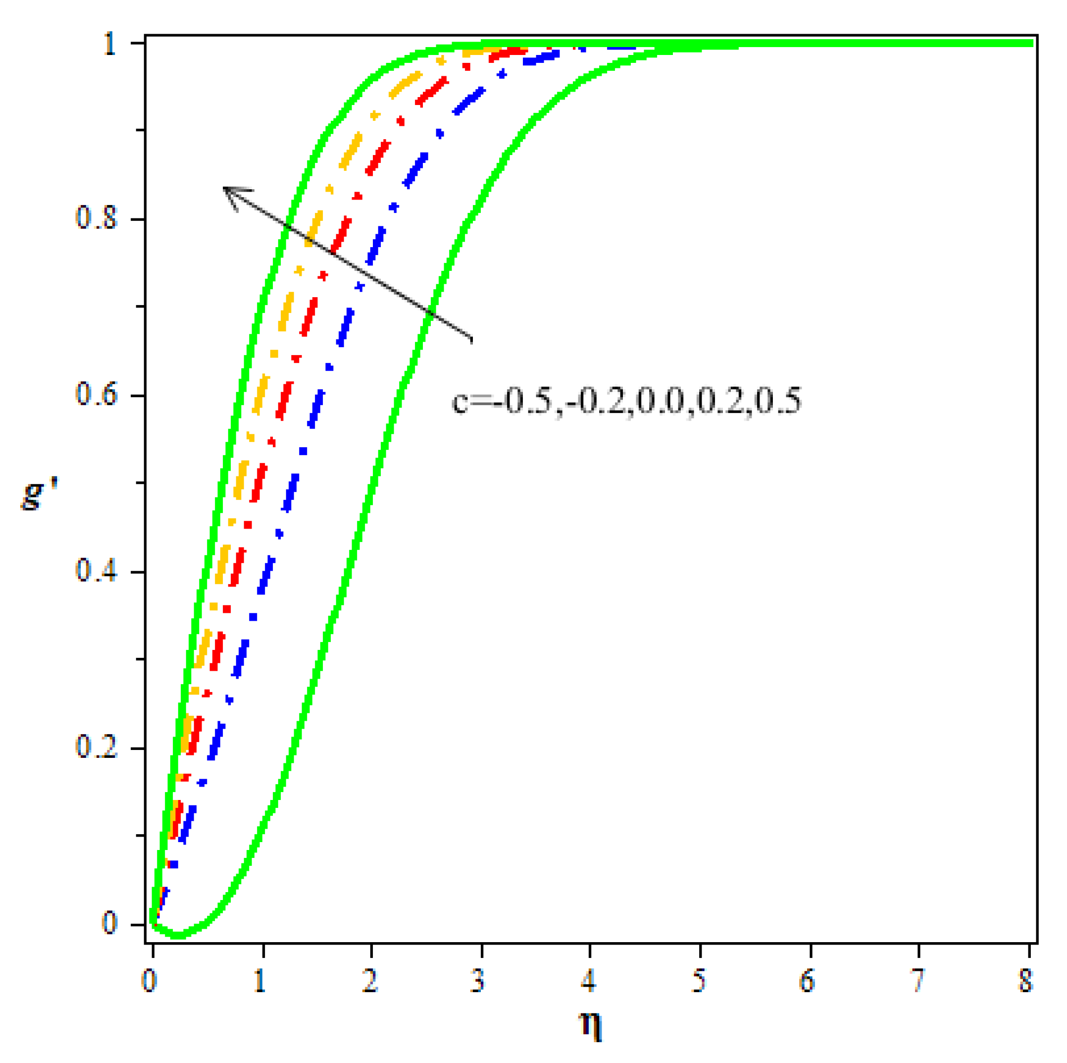
• A rise in the value of the streamline parameter upsurges the flow velocity and decreases the thermal distribution and concentration.
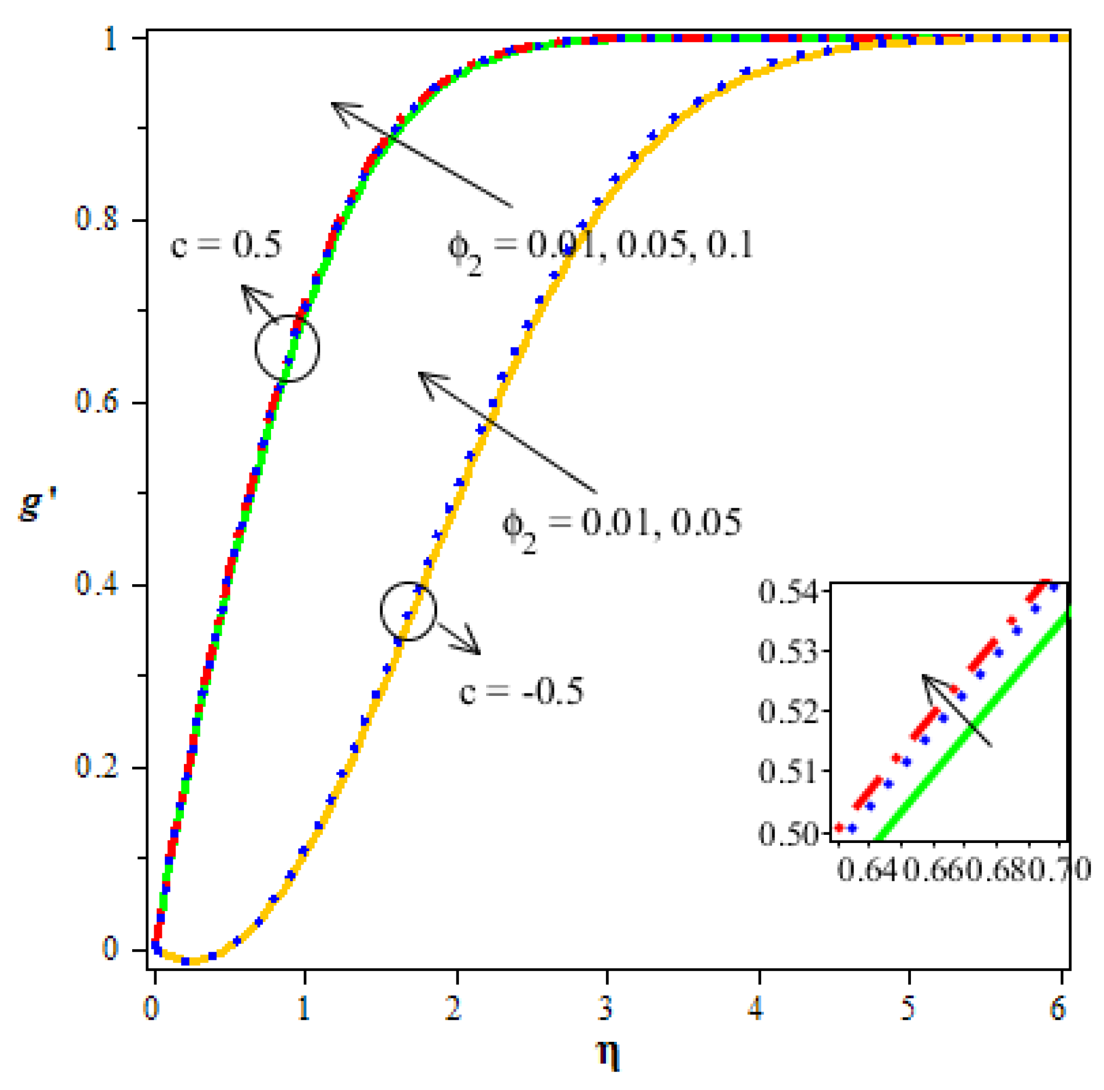
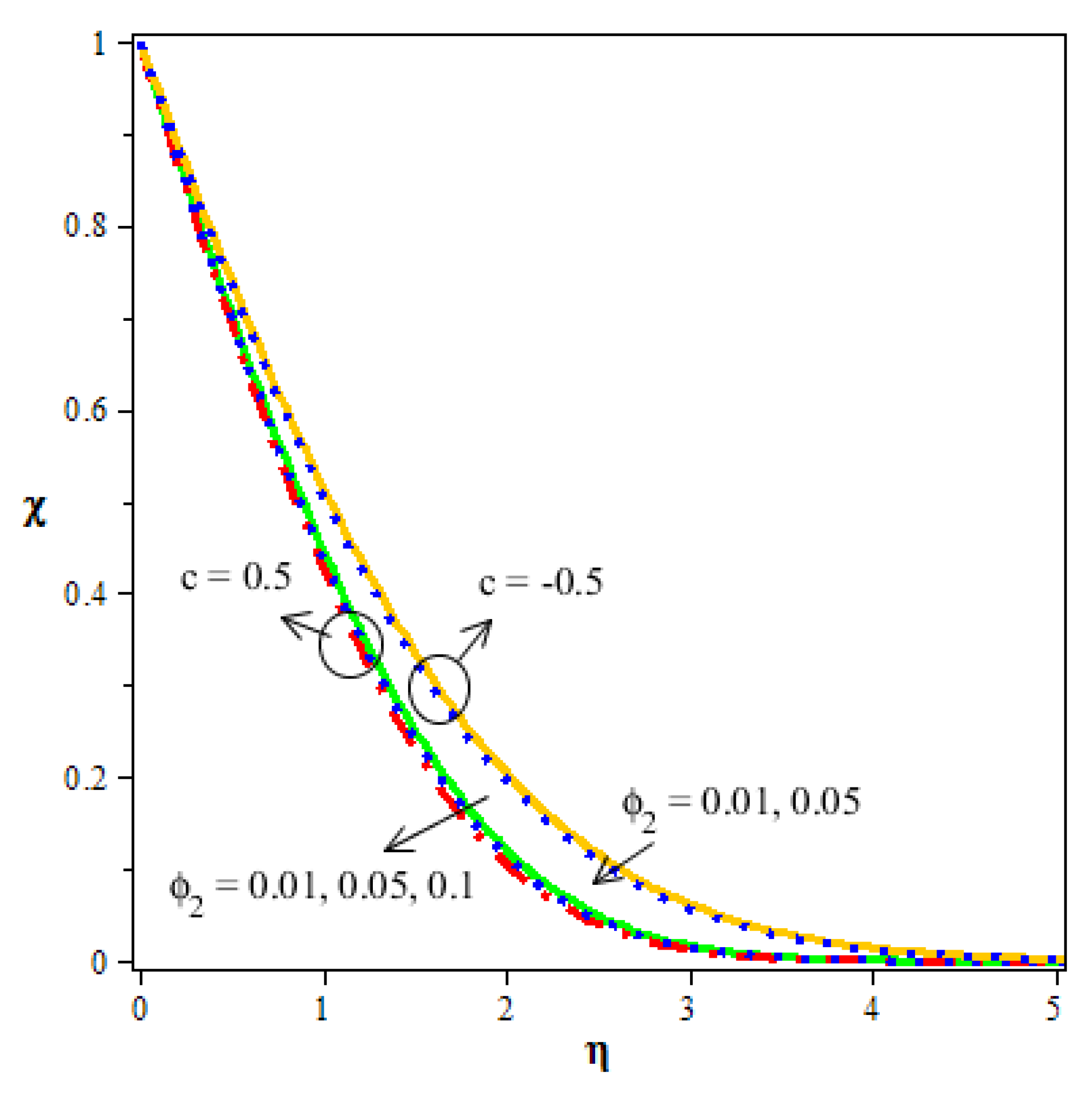
• Better thermal gradient and concentration are seen in the enhancement of volume fraction.
• Boundary layer thickness and concentration are decreased with increase in the Schmidt number.
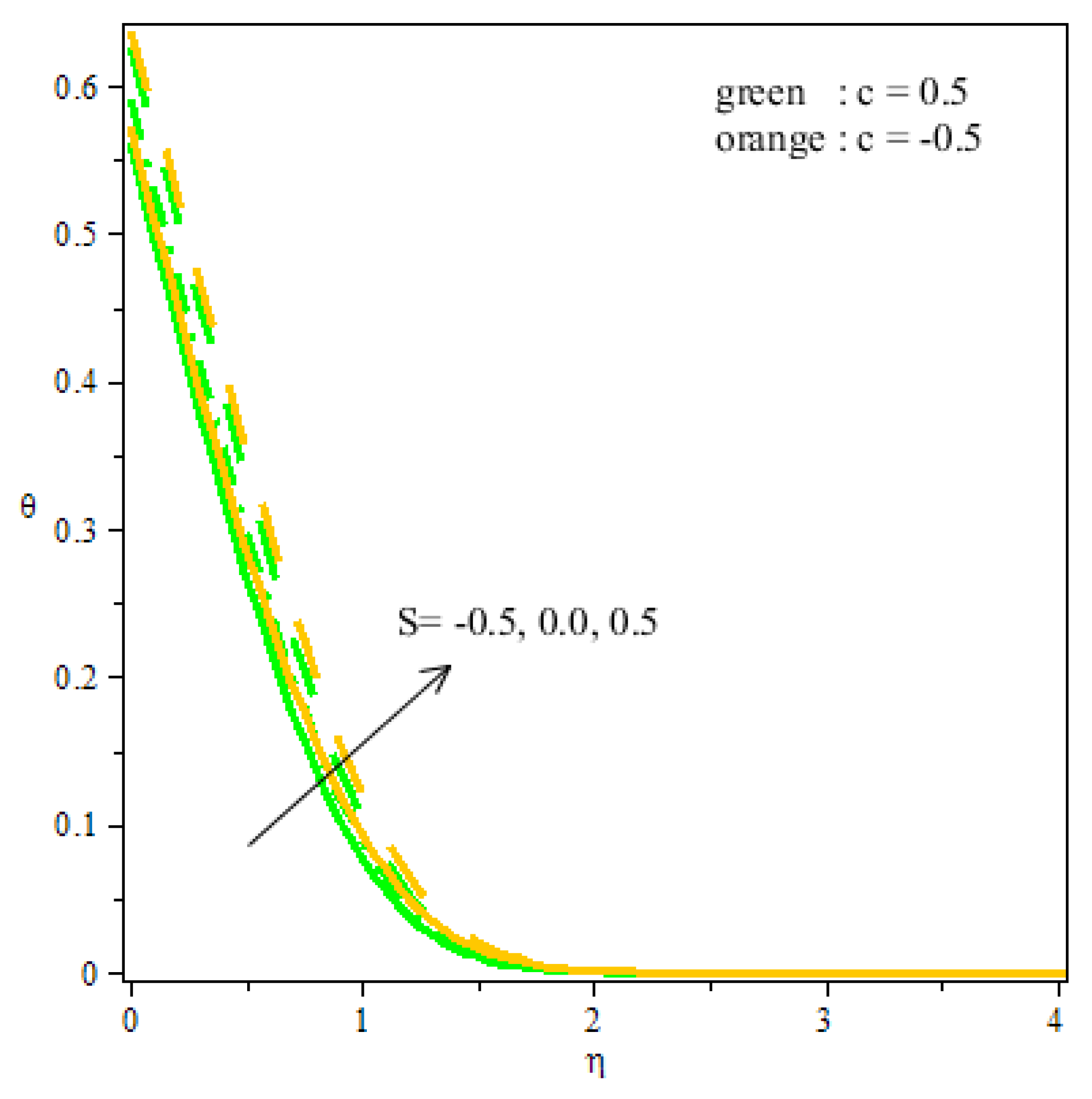
• Thermal distribution and concentration are more in the saddle point than in the nodal point of a hybrid nanofluid.

References

1. Choi, S.U.S.; Eastman, J. Enhancing thermal conductivity of fluids with nanoparticles. In Proceedings of the ASME International Mechanical Engineering Congress and Exposition, San Francisco, CA, USA, 12–17 November 1995; Volume 66. [Google Scholar]
2. Choi, S.U.S. Nanofluids: From Vision to Reality Through Research. J. Heat Transf. 2009, 131, 033106. [Google Scholar] [CrossRef]
3. Koriko, O.K.; Shah, N.A.; Saleem, S.; Chung, J.D.; Omowaye, A.J.; Oreyeni, T. Exploration of bioconvection flow of MHD thixotropic nanofluid past a vertical surface coexisting with both nanoparticles and gyrotactic microorganisms. Sci. Rep. 2021, 11, 16627. [Google Scholar] [CrossRef] [PubMed]
4. Rehman, F.U.; Nadeem, S.; Rehman, H.U.; Haq, R.U. Thermophysical analysis for three-dimensional MHD stagnation-point flow of nano-material influenced by an exponential stretching surface. Results Phys. 2018, 8, 316–323. [Google Scholar] [CrossRef]
5. Fetecau, C.; Shah, N.A.; Vieru, D. General Solutions for Hydromagnetic Free Convection Flow over an Infinite Plate with Newtonian Heating, Mass Diffusion and Chemical Reaction. Commun. Theor. Phys. 2017, 68, 768. [Google Scholar] [CrossRef]
6. Sheikholeslami, M. Magnetic field influence on nanofluid thermal radiation in a cavity with tilted elliptic inner cylinder. J. Mol. Liq. 2017, 229, 137–147. [Google Scholar] [CrossRef]
7. Chamkha, A.J.; Abbasbandy, S.; Rashad, A.M.; Vajravelu, K. Radiation Effects on Mixed Convection over a Wedge Embedded in a Porous Medium Filled with a Nanofluid. Transp. Porous Media 2011, 91, 261–279. [Google Scholar] [CrossRef]
8. Animasaun, I.L.; Shah, N.A.; Wakif, A.; Mahanthesh, B.; Sivaraj, R.; Koriko, O.K. Ratio of Momentum Diffusivity to Thermal Diffusivity: Introduction, Meta-Analysis, and Scrutinization, 1st ed.; Chapman and Hall/CRC: London, UK, 2022. [Google Scholar] [CrossRef]
9. Saeed, M.; Kim, M.-H. Heat transfer enhancement using nanofluids (Al2O3-H2O) in mini-channel heatsinks. Int. J. Heat Mass Transf. 2018, 120, 671–682. [Google Scholar] [CrossRef]
10. Sarkar, J.; Ghosh, P.; Adil, A. A review on hybrid nanofluids: Recent research, development and applications. Renew. Sustain. Energy Rev. 2015, 43, 164–177. [Google Scholar] [CrossRef]
11. Asadi, A.; Alarifi, I.M.; Foong, L.K. An experimental study on characterization, stability and dynamic viscosity of CuO-TiO2/water hybrid nanofluid. J. Mol. Liq. 2020, 307, 112987. [Google Scholar] [CrossRef]
12. Lund, L.A.; Omar, Z.; Khan, I.; Sherif, E.-S.M. Dual Solutions and Stability Analysis of a Hybrid Nanofluid over a Stretching/Shrinking Sheet Executing MHD Flow. Symmetry 2020, 12, 276. [Google Scholar] [CrossRef] [Green Version]
13. Ramesh, G.K.; Shehzad, S.A.; Tlili, I. Hybrid nanomaterial flow and heat transport in a stretchable convergent/divergent channel: A Darcy-Forchheimer model. Appl. Math. Mech. 2020, 41, 699–710. [Google Scholar] [CrossRef]
14. Ramesh, G.; Madhukesh, J. Activation energy process in hybrid CNTs and induced magnetic slip flow with heat source/sink. Chin. J. Phys. 2021, 73, 375–390. [Google Scholar] [CrossRef]
15. Alghamdi, M. Significance of Arrhenius Activation Energy and Binary Chemical Reaction in Mixed Convection Flow of Nanofluid Due to a Rotating Disk. Coatings 2020, 10, 86. [Google Scholar] [CrossRef] [Green Version]
16. Rekha, M.B.; Sarris, I.E.; Madhukesh, J.K.; Raghunatha, K.R.; Prasannakumara, B.C. Activation Energy Impact on Flow of AA7072-AA7075/Water-Based Hybrid Nanofluid through a Cone, Wedge and Plate. Micromachines 2022, 13, 302. [Google Scholar] [CrossRef] [PubMed]
17. Ramesh, G. Analysis of active and passive control of nanoparticles in viscoelastic nanomaterial inspired by activation energy and chemical reaction. Phys. A Stat. Mech. Its Appl. 2020, 550, 123964. [Google Scholar] [CrossRef]
18. Alsaadi, F.E.; Ullah, I.; Hayat, T.; Alsaadi, F.E. Entropy generation in nonlinear mixed convective flow of nanofluid in porous space influenced by Arrhenius activation energy and thermal radiation. J. Therm. Anal. 2019, 140, 799–809. [Google Scholar] [CrossRef]
19. Asma, M.; Othman, W.; Muhammad, T. Numerical study for Darcy–Forchheimer flow of nanofluid due to a rotating disk with binary chemical reaction and Arrhenius activation energy. Mathematics 2019, 7, 921. [Google Scholar] [CrossRef] [Green Version]
20. Ramzan, M.; Gul, H.; Zahri, M. Darcy-Forchheimer 3D Williamson nanofluid flow with generalized Fourier and Fick’s laws in a stratified medium. Bull. Pol. Acad. Sci. Tech. Sci. 2020, 68, 327–335. [Google Scholar]
21. Jagan, K.; Sivasankaran, S.; Bhuvaneswari, M.; Rajan, S. Effect of Non-linear Radiation on 3D Unsteady MHD Nanoliquid Flow over a Stretching Surface with Double Stratification. Trends Math. 2019, 109–116. [Google Scholar] [CrossRef]
22. Nayak, M.K.; Shaw, S.; Chamkha, A.J. 3D MHD Free Convective Stretched Flow of a Radiative Nanofluid Inspired by Variable Magnetic Field. Arab. J. Sci. Eng. 2019, 44, 1269–1282. [Google Scholar] [CrossRef]
23. Irfan, M.; Khan, W.A.; Khan, M.; Gulzar, M.M. Influence of Arrhenius activation energy in chemically reactive radiative flow of 3D Carreau nanofluid with nonlinear mixed convection. J. Phys. Chem. Solids 2019, 125, 141–152. [Google Scholar] [CrossRef]
24. A Alwawi, F.; Alkasasbeh, H.T.; Rashad, A.; Idris, R. Heat transfer analysis of ethylene glycol-based Casson nanofluid around a horizontal circular cylinder with MHD effect. Proc. Inst. Mech. Eng. Part C J. Mech. Eng. Sci. 2020, 234, 2569–2580. [Google Scholar] [CrossRef]
25. Tiwari, R.K.; Das, M.K. Heat transfer augmentation in a two-sided lid-driven differentially heated square cavity utilizing nanofluids. Int. J. Heat Mass Transf. 2007, 50, 2002–2018. [Google Scholar] [CrossRef]
26. Nadeem, S.; Abbas, N. On both MHD and slip effect in micropolar hybrid nanofluid past a circular cylinder under stagnation point region. Can. J. Phys. 2019, 97, 392–399. [Google Scholar] [CrossRef]
27. Tlili, I.; Waqas, H.; Almaneea, A.; Khan, S.U.; Imran, M. Activation Energy and Second Order Slip in Bioconvection of Oldroyd-B Nanofluid over a Stretching Cylinder: A Proposed Mathematical Model. Processes 2019, 7, 914. [Google Scholar] [CrossRef] [Green Version]
28. Shah, N.A.; Wakif, A.; El-Zahar, E.R.; Thumma, T.; Yook, S.-J. Heat transfers thermodynamic activity of a second-grade ternary nanofluid flow over a vertical plate with Atangana-Baleanu time-fractional integral. Alex. Eng. J. 2022, 61, 10045–10053. [Google Scholar] [CrossRef]
29. Rashid, U.; Baleanu, D.; Iqbal, A.; Abbas, M. Shape Effect of Nanosize Particles on Magnetohydrodynamic Nanofluid Flow and Heat Transfer over a Stretching Sheet with Entropy Generation. Entropy 2020, 22, 1171. [Google Scholar] [CrossRef]
30. Manohar, G.R.; Venkatesh, P.; Gireesha, B.J.; Madhukesh, J.K.; Ramesh, G.K. Performance of water, ethylene glycol, engine oil conveying SWCNT-MWCNT nanoparticles over a cylindrical fin subject to magnetic field and heat generation. Int. J. Model. Simul. 2021, 1–10. [Google Scholar] [CrossRef]
31. Mathews, J.H.; Fink, K.D. Numerical Methods Using MATLAB, 3rd ed.; Prentice Hall: Hoboken, NJ, USA, 1998. [Google Scholar]
32. Ramesh, G.; Madhukesh, J.; Das, R.; Shah, N.A.; Yook, S.-J. Thermodynamic activity of a ternary nanofluid flow passing through a permeable slipped surface with heat source and sink. Waves Random Complex Media 2022, 1–21. [Google Scholar] [CrossRef]
33. Gangadhar, K.; Nayak, R.E.; Rao, M.V.S.; Kannan, T. Nodal/Saddle Stagnation Point Slip Flow of an Aqueous Convectional Magnesium Oxide–Gold Hybrid Nanofluid with Viscous Dissipation. Arab. J. Sci. Eng. 2021, 46, 2701–2710. [Google Scholar] [CrossRef]
34. Bhattacharyya, S.; Gupta, A. MHD flow and heat transfer at a general three-dimensional stagnation point. Int. J. Non-Linear Mech. 1998, 33, 125–134. [Google Scholar] [CrossRef]
35. Dinarvand, S. Nodal/saddle stagnation-point boundary layer flow of CuO–Ag/water hybrid nanofluid: A novel hybridity model. Microsyst. Technol. 2019, 25, 2609–2623. [Google Scholar] [CrossRef]
36. Bachok, N.; Ishak, A.; Nazar, R.; Pop, I. Flow and heat transfer at a general three-dimensional stagnation point in a nanofluid. Phys. B Condens. Matter 2010, 405, 4914–4918. [Google Scholar] [CrossRef]
Figure 1. Geometry of the problem.
Mathematics 10 01185 g001
Figure 2. Numerical flow chart.
Mathematics 10 01185 g002
Figure 3. The curve f ( η ) on c .
Mathematics 10 01185 g003
Figure 4. The curve g ( η ) on c .
Mathematics 10 01185 g004
Figure 5. The curve θ ( η ) on c .
Mathematics 10 01185 g005
Figure 6. The curve χ ( η ) on c .
Mathematics 10 01185 g006
Figure 7. The curve f ( η ) on ϕ 2 .
Mathematics 10 01185 g007
Figure 8. The curve g ( η ) on ϕ 2 .
Mathematics 10 01185 g008
Figure 9. The curve θ ( η ) on ϕ 2 .
Mathematics 10 01185 g009
Figure 10. The curve χ ( η ) on ϕ 2 .
Mathematics 10 01185 g010
Figure 11. The curve θ ( η ) on S .
Mathematics 10 01185 g011
Figure 12. The curve θ ( η ) on δ .
Mathematics 10 01185 g012
Figure 13. The curve χ ( η ) on S c .
Mathematics 10 01185 g013
Figure 14. The curve χ ( η ) on β .
Mathematics 10 01185 g014
Figure 15. The curve χ ( η ) on E .
Mathematics 10 01185 g015