Efficient Mining Support-Confidence Based Framework Generalized Association Rules

Abstract

Mining association rules are one of the most critical data mining problems, intensively studied since their inception. Several approaches have been proposed in the literature to extend the basic association rule framework to extract more general rules, including the negation operator. Thereby, this extension is expected to bring valuable knowledge about an examined dataset to the user. However, the efficient extraction of such rules is challenging, especially for sparse datasets. This paper focuses on the extraction of literalsets, i.e., a set of present and absent items. By consequence, generalized association rules can be straightforwardly derived from these literalsets. To this end, we introduce and prove the soundness of a theorem that paves the way to speed up the costly computation of the support of a literalist. Furthermore, we introduce FasterIE, an efficient algorithm that puts the proved theorem at work to efficiently extract the whole set of frequent literalets. Thus, the FasterIE algorithm is shown to devise very efficient strategies, which minimize as far as possible the number of node visits in the explored search space. Finally, we have carried out experiments on benchmark datasets to back the effectiveness claim of the proposed algorithm versus its competitors.

1. Introduction

Discovering association rules is a fundamental and essential subject in data mining and has been extensively investigated since its inception in [1,2]. Over the past few years, the use of association rule mining in varied application scenarios [3,4,5,6,7] have been intensely discussed [8,9]. The idea consists of discovering causal relationships, where the presence of some items suggests that other items follow from them. A typical example of an association rule mining application is the market basket analysis, where the discovered rules can lead to important marketing and strategic management decisions. The process of mining for association rules has two phases:(i) mining for frequent itemsets; and (ii) generating strong association rules from the discovered frequent itemsets.

Traditional association rules mining algorithms were developed to find associations between items present in a transactional database. Nevertheless, in many domains, one might be interested in discovering association rules taking into account the absence of some items to identify conflicting or complementary items. These rules are commonly called generalized association rules [10,11,12]. Nevertheless, considering the negation operator into the association rule framework is the furthest from a straightforward task. Indeed, the challenging issue of mining generalized association rules gave rise to several critical issues:

• When negative items are considered, the length of the transactions increases to reach a value equal to n, where n stands for the number of items in the mined dataset. Since the complexity of standard association rules mining algorithms is very sensitive to the transaction length, these algorithms would break down for such datasets. Indeed, computing supports of itemsets with negation is a very time-consuming step.
• For sparse datasets, a large number of the items are not present in each transaction leading to an overwhelming amount of association rules with negation. Consequently, it is nearly impossible for end-users to comprehend or validate such a high number of the extracted association rules, thereby limiting the usefulness of the mined results.

A large number of researchers have tried to mitigate the search space exploration of the patterns for more efficiently sweeping using the following methods: (i) defining various forms of generalized association rules; (ii) incorporating attribute correlations or rule interestingness measures; and (iii) relying on additional background information concerning the data.

As opposed to this, we propose a new approach staying within the strict bounds of the original support-confidence framework. Our proposal can be intuitive to users, i.e., no additional parameters are required. We usually proceed in two steps to extract generalized association rules: (i) all frequent generalized literalsets are extracted; and (ii) all valid generalized association rules are straightforwardly derived from frequent literalsets. Here the fulfillment of the validity criterion is assessed through the confidence metric that needs to be over a user-defined threshold, called minconf.

A scrutiny of the wealthy number of the related work enables us to draw the following challenging landscape:

• All the surveyed approaches could only extract a particular case of the generalized association rules. This issue is due to the intractability of the extraction of the generalized literaset step.
• The computation of the support of the negative part literaset is the furthest from a trivial task. Even if the computation of the generalized support can be transcripted in terms of the positive part of the literaset, it will lead to a barely bearable computational over-cost burden. Indeed, most of these itemsets are non-frequent, and we need to explicitly delve into the disk-resident database to compute their associated support values.

Keeping these cons in mind, we focus on the first and the most challenging step of generalized association rules mining, i.e., the extraction of frequent literalsets, since it is the most challenging one. To this end, we propose a new algorithm, called FasterIE, for extracting frequent literalsets. Furthermore, we also propose a new method to compute the support of literalsets efficiently. Our approach outperforms its competitors from the literature on benchmark datasets.

The remainder of the paper is organized as follows. In Section 2, we present some basic definitions used throughout the paper. Section 3 reviews the dedicated related work. Section 4 introduces an extended form of association rules that considers the absence of items. Next, we discuss the drawbacks of the naive approach, which uses classical algorithms such as Apriori [13] to extract frequent literalsets in Section 5. Moreover, we introduce a new method for computing the support of a literalset based on the respective supports of its subsets. Section 6 thoroughly details the FasterIE algorithm dedicated to extract the whole set of frequent literalsets. Experimental results are described in Section 7, along with the comparison of FasterIE performances to those of existing algorithms. Finally, Section 8 concludes the paper and points out issues of future work.

2. Basic Concepts and Terminology

This section provides some fundamental notions used in the remainder of the paper. Furthermore, we recall the problem of positive association rule extraction as it has been defined in [13]. The recent past has witnessed a shift in the focus of the association rule mining community, which is now focusing more on an extended form of association rules, callednegative association rules.

Let $\mathcal{I}$ = $\{i_1,i_2,\dots ,i_m\}$ be a set of m items. A transaction, over $\mathcal{I}$, is a couple T = ($tid$, I) where $tid$ is the transaction identifier and I is a set of items such that $I\subseteq \mathcal{I}$. A transaction database $\mathcal{D}$ over $\mathcal{I}$ is a set of transactions over $\mathcal{I}$. A transaction T is said to support a set X if and only if X ⊆ I.

Let X be a subset of $\mathcal{I}$, called positive itemset, containing k items, then X is said to be a positive k-itemset. The absolute support of a positive itemset X is given by Supp(X) = |$tid|$ ($\{tid$, I) $\in \mathcal{D}$, $X\subseteq I\left\}\right|$. If the support of X is greater than or equal to a user-defined minimum threshold minsup, then X is called frequent.

A positive association rule is defined as a correlation between two sets of items [13]. It is sketched as: $R:X\Rightarrow Y$ such that X, $Y\subseteq \mathcal{I}$ and $X\cap Y=\varnothing$. An association rule R is said to be based on the itemset $X\cup Y$ and the itemsets X and Y are called, respectively, premise and conclusion of R.

To assess the validity of an association rule R, two metrics are commonly used [13]: (i) the support: support of the rule R, denoted Supp(R), is given by Supp(X ∪ Y); (ii) the confidence: it expresses the conditional probability to find Y in a transaction containing X. The confidence of the rule R, denoted Conf(R), is given by ${\displaystyle \frac{\mathit{Supp}(X\cup Y)}{\mathit{Supp}(X)}}$. To be valid, an association rule must have its confidence greater than or equal to a user-defined minimum confidence threshold, denoted minconf.

Negative association rules were at first mentioned in [14]. A negative association rule extends positive association rule R: X ⇒ Y to four basic rules $R_1$: $\overline{X}\Rightarrow$ Y, $R_2$: X ⇒ $\overline{Y}$, $R_3$: $\overline{X}\Rightarrow$ $\overline{Y}$ and $R_4$: $X\Rightarrow Y$ where $R_4$ is a positive rule and the other three ones are negative rules where premise or/and conclusion parts represent a negation of an itemset (negative itemset). The semantic meaning of a negative itemset $\overline{X}$ is the non simultaneous presence of items included in X. The extraction of such rules is based on the following observation:

$$\mathit{Supp}(\overline{X}\Rightarrow Y)=\mathit{Supp}(\overline{X}\cup Y)=\mathit{Supp}(Y)-\mathit{Supp}(X\cup Y).$$

Therefore, the support of negative itemsets, on which negative association rules is based, can be deduced from the support of positive itemsets.

3. Related Work

Mining traditional association rules based on frequent itemsets have been extensively studied since their introduction by [13]. However, mining negative association rules have been less often addressed.

The idea of mining negative association rules was firstly presented in [14] where the authors introduced the concept of excluding associations. Indeed, they presented a versatile method to find associations of the form $AB\overline{C}\Rightarrow D$, where $AB\Rightarrow D$ is not maintained due to a low confidence value. This approach permits the extraction of a subset of generalized association rules where their premise part contains only one negative literal.

We discuss the main approaches dedicated to extract negative association rules in the following.

3.1. The Gen-Neg-Rules Algorithm

Savasere et al. proposed an algorithm to mine strong negative association rules by combining frequent itemsets and domain knowledge to form taxonomy [15]. Their basic assumption was that items from the same product family are expected to have similar types of interaction with other items. The authors use the item taxonomy to determine the expected support of an itemset. If the actual support of an itemset $X\cup Y$ is considerably lower than expected, the authors conclude that a negative association between X and Y may be of interest. The authors proposed the following definitions:

Definition 1.

Let a formal context $\mathcal{K}$ = ($\mathcal{O},\mathcal{I},\mathcal{R}$) such that $\mathcal{O}$ represents a finite set of objects (or transactions), $\mathcal{I}$ represents a finite set of attributes (or items) and $\mathcal{R}$ is a binary relation (i.e, $\mathcal{R}$ ⊆ $\mathcal{O}$ × $\mathcal{I}$). Let $\mathcal{T}$ a taxonomy, associated to $\mathcal{K}$, containing a set $\mathcal{J}$ of items. Let X a subset of $\mathcal{J}$, X is said to be a multi-level itemset if and only if $\nexists j\in X$ such that j is descendant of an item $j^{\prime }\in X$. The support of a multi-level itemset X is computed as follows: Supp(X) = |($\{o_i\in$$\mathcal{O}|\forall$$x_j\in$ X, ($x_j$, $o_i$) ∈ $\mathcal{R}$∨ ($x_n$, $o_i$) ∈ $\mathcal{R}$, $x_n$∈ descendant($x_j$)})|.

Definition 2.

Let X and Y be two valid interesting multi-level itemsets. A negative association rule R: $X\Rightarrow Y$, is valid if and only if its value of interestingness RI is at least equal to MinRI, where RI is equal to the following:

$$RI={\displaystyle \frac{\epsilon [\mathit{Supp}(X\cup Y)]-\mathit{Supp}(X\cup Y)}{\mathit{Supp}(X)}}$$

The Gen-Neg-Rules algorithm relies on the following steps:

• Extracting the multi-level itemsets: First, the authors proposed to extract multi-level itemsets based on Definition 1.
• Extracting the interesting multi-level itemsets: Let X be a frequent multi-level itemset. The set of interesting multi-level itemsets based on X is obtained by replacing some items of X by their parents or their siblings. A valid interesting multi-level itemsets should have a deviation value (deviation(X) = $\epsilon$[Supp(X)] − Supp(X)) which is greater or equal to minsup × MinRI, such that MinRI is a threshold of interestingness fixed by the user and $\epsilon$[Supp(X)] denotes the expected support of X. Three cases must be distinguished whenever we have to compute the expected support of an interesting multi-level itemset:

  1st case:

  Let X = {p, q, …, t} be a frequent multi-level itemset and Y = {p${}_{\wedge }$, q${}_{\wedge }$, …, t${}_{\wedge }$} be a candidate interesting multi-level itemset such that p${}_{\wedge }$, q${}_{\wedge }$, …, t${}_{\wedge }$ are respectively, the children of p, q, …, t in the taxonomy. The expected support of Y is then equal to:

  $${\displaystyle \epsilon \left[\mathit{Supp}(Y)\right]=\frac{\mathit{Supp}(X)\times \mathit{Supp}(p_{\wedge })\times \mathit{Supp}(q_{\wedge })\times \dots \times \mathit{Supp}(t_{\wedge })}{\mathit{Supp}(p)\times \mathit{Supp}(q)\times \dots \times \mathit{Supp}(t)}}$$

  2nd case:

  Let X = {p, q, r, …, t} be a frequent multi-level itemset and Y = {p, q, r${}_{\wedge }$, …, t${}_{\wedge }$} be a candidate interesting multi-level itemset such that r${}_{\wedge }$, …, t${}_{\wedge }$ are respectively, the children of r, …, t in the taxonomy. The expected support of Y is then equal to:

  $${\displaystyle \epsilon \left[\mathit{Supp}(Y)\right]=\frac{\mathit{Supp}(X)\times \mathit{Supp}(r_{\wedge })\times \dots \times \mathit{Supp}(t_{\wedge })}{\mathit{Supp}(r)\times \dots \times \mathit{Supp}(t)}}$$

  3rd case:

  Let X = {p, q, r, …, t} be a frequent multi-level itemset and Y = {p, q, r${}_{<}$, …, t${}_{<}$} be a candidate interesting multi-level itemset such that r${}_{<}$, …, t${}_{<}$ are respectively, siblings of r, …, t in the taxonomy. The expected support of Y is then equal to:

  $${\displaystyle \epsilon \left[\mathit{Supp}(Y)\right]=\frac{\mathit{Supp}(X)\times \mathit{Supp}(r_{<})\times \dots \times \mathit{Supp}(t_{<})}{\mathit{Supp}(r)\times \dots \times \mathit{Supp}(t)}}$$

• Extracting the negative association rules: The authors redefined negative association rules based on Definition 2. Hence, negative association rules can be generated once valid, and interesting multi-level item sets are extracted.

• At a glance, the Gen-Neg-Rules algorithm is intuitively appealing. Nevertheless, it has several limitations. First, it assumes that an item taxonomy is available, making it difficult to generalize the proposed approach. Second, it discovers negative associations by computing item sets’ expected support using the item taxonomy’s immediate parent-child or sibling relationships. Finally, it does not infer the expected support for itemsets unrelated to immediate parent-child or sibling relationships.

3.2. The DI-Apriori Algorithm

Morzy added the $join$ measure allowing to assess the rarity of an itemset [16]. In addition, the author introduced the notion of dissociative itemset defined as follows:

Definition 3.

Let maxjoin a user-defined maximal threshold of the join measure, where $minsup>maxjoin$. An itemset Z is said to be dissociative, if and only if:

• $Supp(Z)\le maxjoin$,
• ∃ X and Y, such that $X\cap Y=\varnothing$, $X \cup$ $Y=Z$, $Supp(X)\ge minsup$ and $Supp(Y)\ge minsup$.

Plainly speaking, given a dissociative itemset Z = $X\cup Y$, then Z represents that both X and Y are frequent and X rarely occurs with Y. In addition, to limit the exploration of the search space, Morzy suggested extracting a subset of dissociative itemsets called minimal dissociative itemsets, defined as follows:

Definition 4.

A dissociative itemset $X\cup Y$ is minimal if and only if it does not exist a dissociative itemset $X^{\prime }\cup Y^{\prime }$, such that $X^{\prime }\subset X$ and $Y^{\prime }$$\subset Y$.

To extract the generalized association rules, Morzy introduced the DI-Apriori algorithm, which proceeds in four steps:

• Extracting the positive association rules: First, the algorithm generates the set of frequent dissociative itemsets like Apriori algorithm [13]. Then it generates the positive association rules.
• Extracting the minimal dissociative itemsets: It was argued in [16] that an itemset X belonging to the negative border $B{d}^{-}$ (the negative border denoted $B{d}^{-}$, contains infrequent itemsets whose all respective subsets are frequent) is either a candidate dissociative itemset or a subset of a candidate dissociative itemset. Based on this observation, the negative border $B{d}^{-}$ is examined and all itemsets with support value lower than $maxjoin$ are added to the set of valid minimal dissociative itemsets $\mathcal{D}$. The remaining itemsets in the negative border form the seed set of candidate minimal dissociative itemsets $\mathcal{C}$. Each itemset $X\cup Y$ in $\mathcal{C}$ is extended with a frequent 1-itemsets i. If ($X\cup i$) and ($Y\cup i$) are both frequent and ($X\cup Y\cup i$) is also infrequent, then ($X\cup i)X\cup Y\cup i$) is a candidate minimal dissociative itemset. If the support of $(X\cup Y\cup i)$ is lower than $maxjoin$, then $(X\cup Y\cup i)$ is added to $\mathcal{D}$. Otherwise, it is added to $\mathcal{C}$.
• Derivating the dissociative itemsets: Based on the set $\mathcal{D}$, the algorithm derives the whole set of the remaining dissociative itemsets. Then, the algorithm derives the remaining dissociative itemsets, for each minimal dissociative itemset $X\cup Y$, by replacing X and Y by their respective frequent supersets.
• Generating the negative association rules: Once the dissociative itemsets are extracted, DI-Apriori derives association rules of the form $X\nRightarrow Y$ with respect to the provided minconf threshold.

The author proposed an approach permitting to generate, on the one hand, positive association rules like the Apriori algorithm [13]. On the other hand, the author added the $maxjoin$ threshold to belittle the number of infrequent itemsets and defined dissociative itemsets. In addition, this approach allows extracting a concise representation of itemsets. The remaining dissociative itemsets are derived straightforwardly from these minimal dissociative itemsets. However, it is worth mentioning that this operation is computationally expensive. Hence, extracting a generic basis of association rules from minimal dissociative item sets is more appropriate. Then, the remaining (redundant) rules can be derived from the user’s demand.

3.3. The Positive and Negative Associations Algorithm

Wu et al. presented an Apriori-based framework for mining generalized association rules [11], which focuses on the rule interest measure [17]. Indeed, in the latter reference, it was argued that a rule $X\Rightarrow Y$ is not worth of interest whenever $Supp(X\cup Y)-Supp(X)\times Supp(Y)=0$. An interpretation of this proposition is that a rule is not interesting whenever its premise and consequent are approximately independent.

Definition 5.

To put at work the concept introduced by Piatetsky-Shapiro, Wu et al. defined an interestingness measure, called interest $(X,Y)=|Supp(X\cup Y)$ − $Supp(X)\times Supp(Y)|$. Thus, given a minimum interestingness threshold $minint$, if interest($X,Y)\ge minint$, then the rule X ⇒ Y is of potential interest, and $X\cup Y$ is referred to as a potentially interesting itemset.

Aiming at extracting generalized association rules, Wu et al. proposed an algorithm, called Positive And Negative Associations, operating into two steps:

• Extracting the frequent and infrequent itemsets of interest: The authors maintain two sets: (i) $\mathcal{FI}$: the set of frequent itemsets; and (ii) $\mathcal{INF}$: the set of infrequent itemsets. First, the algorithm generates ${\mathcal{FI}}_1$ and ${\mathcal{INF}}_1$ containing, respectively, frequent 1-itemsets and infrequent 1-itemsets. After that, for each $k\ge 2$, two steps are required:

  -

  The algorithm generates ${\mathcal{C}}_k$ containing all candidate k-itemsets where each k-itemset in ${\mathcal{C}}_k$ is generated by two frequent itemsets in ${\mathcal{FI}}_{k-1}$. After determining the support of each itemset in ${\mathcal{C}}_k$, the algorithm inserts into ${\mathcal{FI}}_k$ frequent k-itemsets and inserts ${\mathcal{C}}_k$ − ${\mathcal{FI}}_k$ into ${\mathcal{INF}}_k$.

  -

  For each element of ${\mathcal{FI}}_k$ or ${\mathcal{INF}}_k$, the algorithm removes all itemsets that do not meet the minint threshold. Let I ∈ ${\mathcal{FI}}_k$ or I∈${\mathcal{INF}}_k$, ∀X and Y such that $X\cup Y=I$, the algorithm checks whether interest(X, Y) $\le minint$.

• Derivating the generalized association rules of interest: based on Piatetsky-Shapiro’s argument [17], the authors introduced a conditional-probability increment ratio function for a pair of itemsets X and Y, denoted by Cpir as follows:

  $${\displaystyle \mathit{Cpir}(X|Y)=\frac{\mathit{Supp}(X|Y)-\mathit{Supp}(Y)}{1-\mathit{Supp}(Y)} \mathrm{if} \mathit{Supp}(X|Y)\ge \mathit{Supp}(Y) \mathrm{and} \mathit{Supp}(Y)\ne 1,}$$

  or

  $${\displaystyle \mathit{Cpir}(X|Y)=\frac{\mathit{Supp}(X|Y)-\mathit{Supp}(Y)}{\mathit{Supp}(Y)} \mathrm{if} \mathit{Supp}(X|Y)<\mathit{Supp}(Y) \mathrm{and} \mathit{Supp}(Y)\ne 0.}$$
  To derive association rules, the authors proposed an algorithm which generates positive association rules of interest based on itemsets of $\mathcal{FI}$. In addition, if Cpir($Y|X$) ≥ minconf, Y$\Rightarrow X$ is extracted as a valid rule of interest. If Cpir($X|Y$ ≥ minconf, $X\Rightarrow Y$ is extracted as a valid rule of interest. For each itemset I in $\mathcal{INF}$, the algorithm generates negative association rules of interest based on I if interest(X, $\overline{Y}$) ≥ minint. If Cpir($\overline{Y}$, X) ≥ minconf, $\overline{Y}$ ⇒ X is extracted as a valid rule of interest. If Cpir (X, $\overline{Y}$) ≥ minconf, X ⇒ $\overline{Y}$ is extracted as a valid rule of interest ($\overline{X}$ ⇒ $\overline{Y}$ is also generated as a valid rule if it fulfills both the Cpir and minint thresholds).
  The proposed approach’s main idea is to extract positive association rules from frequent itemsets and negative association rules from infrequent itemsets. However, this strategy has substantial problems since the proposed algorithm cannot generate all valid positive and negative association rules. Indeed, the interest function used in this algorithm for pruning itemsets does not have a downward closure property like support. Furthermore, for each iteration k, the set ${\mathcal{INF}}_k$ is deduced from ${\mathcal{FI}}_k$. Hence, the algorithm cannot generate all infrequent itemsets.

3.4. The Positive and Negative Correlated Associations Algorithm

Antonie and Zaïane considered a framework [18] that adds to the support-confidence measures the correlation coefficient [19] allowing to assess the strength of the linear relationship between two itemsets. For example, let X and Y be two itemsets, then the correlation coefficient is given by the following formula:

$${\displaystyle \mathit{correlation}(X,Y)=\frac{\mathit{Supp}(X\cup Y)-\mathit{Supp}(X)\times \mathit{Supp}(Y)}{\sqrt{\mathit{Supp}(X)\times (1-\mathit{Supp}(X))\times \mathit{Supp}(Y)\times (1-\mathit{Supp}(Y))}}}$$

The authors proposed an algorithm that combines the phase of itemsets extraction and that of association rules derivation to extract generalized association rules. Indeed it generates the relevant rules on the fly while analyzing the correlations within each candidate itemset. Initially, the algorithm determines the set of frequent 1-itemsets. Instead of joining frequent (k − 1)-itemsets to obtain candidates of iteration k, the algorithm proceeds by joining the frequent itemsets of iteration (k − 1) with the frequent 1-itemsets. This permits extending the set of candidate itemsets and can analyze the correlation of more item combinations. For each candidate itemset I, all combinations of itemsets X $\cup Y$ such that $X\cup Y=I$ are extracted. Then, for each itemset $X\cup Y$, the algorithm computes the correlation coefficient between X and Y. In this phase, two cases arise:

1st case: 

If the correlation coefficient measure is positive and greater than or equal to a correlation threshold, then an association rule $X\Rightarrow Y$ is generated. This association rule is valid if and only if its support and its confidence are greater than or equal to, respectively, minsup and minconf. If the support is less than minsup, then the rule $\overline{X}\Rightarrow$$\overline{Y}$ is generated whenever it satisfies the minsup and minconf constraints.

2nd case: 

Suppose the correlation coefficient measure is negative while having an absolute value greater than or equal to the correlation threshold. In that case, both rules $\overline{X}\Rightarrow Y$ and X ⇒ $\overline{Y}$ are derived if they both satisfy minsup and minconf thresholds.

3.5. The Pnar Algorithm

Cornelis et al. proposed an algorithm, called Pnar [20] based on the following definitions:

Definition 6.

Let ${\mathcal{DR}}_k$ = $\{R_1$, …, $R_n\}$ be the set of association rules that can be extracted from a transaction database $\mathcal{D}$. A rule $R_1$: ${\overline{X}}_1\Rightarrow Y\in {\mathcal{DR}}_k$ is said to be more general than $R_2:{\overline{X}}_2$$\Rightarrow Y\in {\mathcal{DR}}_k$, denoted $R_1$≺$R_2$, if and only if $X_1\subset X_2$.

Definition 7.

$\mathcal{MR}$ = {$R_i$ ∈ ${\mathcal{DR}}_k$|∄$R_j$ ∈ ${\mathcal{DR}}_k$, $R_j$≺$R_i\}$

The Pnar alorithm proceeds in two steps:

• Extracting the frequent itemsets: This step is built up conceptually around a partition of the itemsets space into four sets:
  • First, the algorithm extracts the set of frequent positive itemsets $P1$.
  • For each frequent positive itemset I in $P1$, the algorithm inserts $\overline{I}$ into $P2$.
  • The algorithm constructs the set $P3$ containing itemsets, which are conjunctions of two negative itemsets of $P2$.
  • Based on $P1$ and $P2$, the algorithm generates frequent itemsets, which are conjunctions of an itemset of $P1$ and an itemset of $P2$.
• Generating the generalized association rules: Based on the four classes of itemsets already extracted, Cornelis et al. proposed to extract a subset of association rules from which the whole set of redundant rules can be deduced. Indeed, Cornelis et al. defined the redundancy of a rule. Hence, using Definition 6, the authors introduced a subset of association rules, called set of minimal rules and denoted $\mathcal{MR}$ according to Definition 7. Once $P1$, $P2$, $P3$, and $P4$ are extracted, the algorithm generates first positive association rules from $P1$. Second, for each itemset $\overline{X}\cup \overline{Y}$ of $P3$, The Pnar algorithm derives each minimal association rule R: $\overline{X}$ ⇒ $\overline{Y}$ whenever its confidence value is at least equal to minconf. Third, for each itemset $\overline{X}\cup Y$ of $P4$, the algorithm generates $\overline{X}\Rightarrow Y$ and $X\Rightarrow \overline{Y}$ if they fulfill the minconf threshold.

It is worthy of mention that the Pnar algorithm cannot generate all possible negative itemsets. Indeed, the authors deduced $P2$, $P3$, and $P4$ from the set of frequent positive itemsets $P1$. Furthermore, the authors do not provide any inference mechanism to derive, without information loss, redundant association rules from those retained.

3.6. The Apriori FISinFIS Algorithm

Mahmood et al. proposed a set of algorithms for discovering positive and negative association rules simultaneously among frequent and infrequent itemsets from textual datasets along with three different phases [12].

• In the first phase, the authors proposed an algorithm called Apriori FISinFIS that generates all frequent (FIS) and infrequent (inFIS) itemsets of interest (i.e., having support and confidence greater than a predefined minSupp and minConf). Infrequent itemset (inFIS) generation is of great importance in generating negative association rules and tracking essential implications/associations, which would have been missed when mining only positive association rules.
• In the second phase, another algorithm is defined to generate positive and negative association rules with greater confidence than the user-defined threshold and lift greater than 1. The extracted associations are considered as valid positive and negative association rules, respectively.
• Negative association rules are captured among frequent itemsets (FIS). However, positive associations are extracted among the infrequent itemsets (inFIS).

The extraction of positive and negative rules is based on the following equations [12]:

$$\mathit{Lift}(X\Rightarrow Y)=\frac{\mathit{P}(X\cup Y)}{\mathit{P}(X)\mathit{P}(Y)}$$

$$\mathit{Supp}(\overline{X})=1-\mathit{Supp}(X)$$

$$\mathit{Supp}(X\cup \overline{Y})=\mathit{Supp}(X)-\mathit{Supp}(X\cup Y).$$

$$\mathit{Conf}(X\Rightarrow \overline{Y}{\displaystyle )}=1-\mathit{Conf}(X\Rightarrow Y)=\frac{\mathit{P}(X\overline{Y})}{\mathit{P}(X)}$$

$$\mathit{Supp}(\overline{X}\cup Y)=\mathit{Supp}(Y)-\mathit{Supp}(Y\cup X).$$

$$\mathit{Conf}(\overline{X}\Rightarrow Y)=\frac{\mathit{Supp}(\overline{X}\cup Y)}{\mathit{Supp}(\overline{X})}$$

$$\mathit{Supp}(\overline{X}\cup \overline{Y})=1-\mathit{Supp}(X)-\mathit{Supp}(Y)+\mathit{Supp}(X\cup Y).$$

$$\mathit{Conf}(\overline{X}\Rightarrow \overline{Y})=\frac{1-\mathit{Supp}(X)-\mathit{Supp}(Y)+\mathit{Supp}(X\cup Y)}{1-\mathit{P}(X)}=\frac{\mathit{Supp}(\overline{X}\cup \overline{Y})}{\mathit{Supp}(\overline{X})}$$

To the best of our knowledge, no algorithm of the scrutinized approaches is grounded to extract the generalized association rules as defined in Section 4. Indeed, in [18], Antonie and Zaïane acknowledged that their approach was not general enough to capture the whole set of generalized association rules. The authors constrained themselves by extracting a subset of generalized association rules. The premise or the conclusion is a conjunction of only negative literals or conjunction of only positive literals. In addition, in [14], the authors extracted a subset of generalized association rules where only the premise part can contain one negative literal.

4. Efficient Extraction of Generalized Association Rules

We usher this section by defining an extended form of association rules, called generalized association rules, which takes into account the presence as well as the absence of the items.

Let $\mathcal{I}$ = $\{i_1,i_2,\dots ,i_m\}$ be a set of items and $\mathcal{L}$ = $\mathcal{I}\cup \left\{\overline{i}\right|i$ ∈ $\mathcal{I}\}$ be the set of literals, such that a literal is an item i (said a positive literal) or its opposite $\overline{i}$ (said a negative literal). Let L be a subset of $\mathcal{L}$ containing k non opposite literals, then L is called k-literalset. Let L be a k-literalset composed of p positive literals and (k − p) negative literals. Then, L is said to be a p-positive literalset, i.e., a ($k-p$)-negative literalset. We denote by PosVar$(L)$, PosPart$(L)$ and NegPart$(L)$, respectively, the positive variation, the set of the positive literals, and the set of the negative literals of L. Formally, these three notions are defined as follows:

Definition 8.

Let L be a literalset such that L = {$i_1$, $i_2$, …, $i_p$, ${\overline{j}}_1$, ${\overline{j}}_2$, …, ${\overline{j}}_l$}.

$$\mathrm{POSVAR}(L)=\{i_1,i_2,\dots ,i_p,j_1,j_2\dots ,j_l\}.$$

$$\mathrm{POSPART}(L)=\{i_1,i_2,\dots ,i_p\}.$$

$$\mathrm{NEGPART}(L)=\{{\overline{j}}_1,{\overline{j}}_2,\dots ,{\overline{j}}_l\}.$$

Let a transaction database $\mathcal{D}$ over a set of items $\mathcal{I}$. A transaction T of $\mathcal{D}$ is said to support a literalset L whenever it supports PosPart$(L)$ and does not contain any opposite literal of NegPart$(L)$, i.e.,

$$\mathit{Supp}(L)=\left|\right\{tid|(tid,I)\in \mathcal{D},\mathrm{POSPART}(L)\subseteq I \mathrm{and} \forall \overline{j}\in \mathrm{NEGPART}(L),j\notin I\}|.$$

A literalset L is said to be frequent if and only if its support is at least equal to a minimum threshold minsup. It is worth underscoring that the set $\mathcal{FL}$ of frequent literalsets is a downward closure, i.e., equipped by the anti-monotone property, as it is the case for the set of frequent itemsets. Indeed, if $L\in \mathcal{FL}$, ∀$L_1\supseteq L$, $L_1$ is also frequent. Conversely, if $L\notin \mathcal{FL}$, $\forall L_1\supset L$, $L_1$ is not frequent.

Example 1.

Let us consider the transaction database, shown in

Table 1. A transaction database $\mathcal{D}$.

Tid	Items
$t_1$	ae
$t_2$	ace
$t_3$	abd
$t_4$	bce
$t_5$	ae

, over the set of items $\mathcal{I}$ = $\{a,b,c,d,e\}$. We have $a\overline{b}\overline{c}$ is a 3-literalset and it also is a 1-positive literalset. Its support value is equal to $\mathit{Supp}$ ( $a\overline{b}\overline{c}$ ) = 2, while PosVar ( $a\overline{b}\overline{c}$ ) = $abc$, PosPart ( $a\overline{b}\overline{c}$ ) = a and NegPart ( $a\overline{b}\overline{c}$ ) = $\overline{b}\overline{c}$. Let minsup = 2, $a\overline{b}\overline{c}$ is then a frequent literalset. All its subsets are then also frequent literalsets. For example, $\mathit{Supp}(a\overline{b})=3\ge 2$.

We define a generalized association rule as a correlation between two literalsets and having the following form $R:L_1\Rightarrow L_2$ where $L_1$, $L_2\subseteq \mathcal{L}$ and $L_1\cap L_2=\varnothing$. A generalized association rule is said to be valid if and only if its support value, i.e., the support of $L_1\cup L_2$, is at least equal to minsup and its confidence is at least equal to $minonf$.

5. Efficient Computation of the Support of Literalsets

The extraction process of generalized association rules can be split into two steps as follows:

• Extract frequent literalsets;
• Derive valid generalized association rules: this step is the least computational. Indeed, for each frequent literalset L, we derive all possible combinations $L_1$ and $L_2$, such that $L_1$, $L_2\subseteq L$ and $L_1\cap L_2=\varnothing$, for which the minconf constraint is fulfilled.

For this purpose, the remainder of this section is devoted to the tricky and challenging task of extracting frequent literalsets. We usher this development by paying heed to discussing the opportunity of a straightforward naive Brute-force approach.

5.1. A Naive Brute-Force Approach

A naive brute-force approach consists of augmenting each transaction of the original dataset with new item identifiers representing the absence of each item from a transaction and, then, straightforwardly applying a classical algorithm such as Apriori [13] on a generalized transaction datasbase as the one given in

Table 2. A generalized transaction database $\mathcal{D}$.

Tid	Items
$t_1$	a$\overline{b}$$\overline{c}$$\overline{d}$e
$t_2$	a$\overline{b}$c$\overline{d}$e
$t_3$	ab$\overline{c}$d$\overline{e}$
$t_4$	$\overline{a}$bc$\overline{d}$e
$t_5$	a$\overline{b}$$\overline{c}$$\overline{d}$e

.

Nevertheless, this approach was shown to be inefficient, especially during the step dedicated to the computation of literalsets supports [21]. Indeed, to compute supports of the candidate k-literalsets, the algorithm has to check for each k-subset of a transaction $T=(tid,L)$ (L is a set of literals, such that $L\subseteq \mathcal{L}$.) whether it belongs to the set of the candidate k-literalsets. Since the length of each transaction was increased to reach a value equal to $n=\left|\mathcal{I}\right|$, then the number of the k-subsets that we have to check rockets considerably. The computation of literalsets supports will be a very time-consuming and intractable step.

5.2. Toward an Efficient Computation the Support of a Literalset

As underscored before, extracting generalized association rules from the extended transaction database is impractical whenever the classical mining approach is used. Thus, it would be interesting to devise a solution that permits to extraction of generalized association rules directly from the original transaction database. Nevertheless, computing supports of literalsets becomes problematic. In other words, how can we compute the support of a literalset from transactions which contain only the present items? In such a situation, the inclusion-exclusion principle can offer an efficient option. Indeed, this well-known principle was of extensive use in many enumeration problems [22]. Moreover, this principle was used in [21,23] to compute the support of a literalset. Given a literalset $L=\{i_1,\dots ,i_m,{\overline{j}}_1,\dots ,{\overline{j}}_n\}$, then its support is computed as follows:

$$\mathit{Supp}(L)=\sum _{S\subseteq \{j_1,\dots ,j_n\}}{(-1)}^{\left|S\right|}\times \mathit{Supp}(\{i_1,\dots ,i_m\}\cup S)$$

(1)

Example 2.

Let $a\overline{b}\overline{c}\overline{d}$ be a literalset. Then, its support is computed as follows:

$$\mathit{Supp}(a\overline{b}\overline{c}\overline{d})=\mathit{Supp}(a)-\mathit{Supp}(ab)-\mathit{Supp}(ac)-\mathit{Supp}(ad)+\mathit{Supp}(abc)+\mathit{Supp}(abd)+\mathit{Supp}(acd)-\mathit{Supp}(abcd).$$

Hence, we notice that the support of a literalset L can be deduced by only considering the supports of positive itemsets. Indeed, the support of a literalset L is determined from the support of PosVar(L) and those of the subsets of NegPart(L). However, it is worth putting forward that positive itemsets, of need to compute the support of a literalset, are not necessarily found to be frequent ones. Consequently, as a flagrant con, these approaches [21,23] need to perform supplementary accesses to the dataset to count the supports of these infrequent positive itemsets. To tackle such an insufficiency, Boulicaut et al. proposed a potential solution, which consists of providing an approximate value of the support of a literalset by ignoring infrequent positive itemsets [21]. Thus, the more positive itemsets are infrequent, the more non-scalable this approach is.

In the following, we introduce a new theorem that reduces the number of accesses to the database. Nevertheless, first, we intuitively illustrate the driving idea through an example.

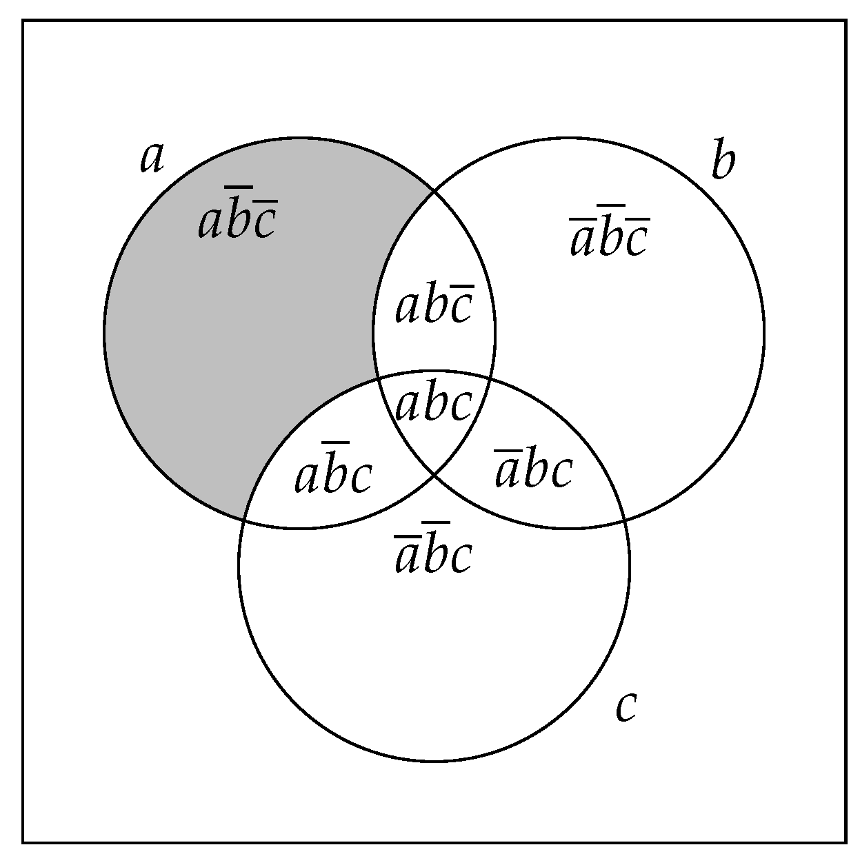
Example 3.

Let us consider the transaction database $\mathcal{D}$ depicted by Table 1. Figure 1 shows transactions that contain the literal a, respectively, b and c. At a glance, we can notice that:

$$\mathit{Supp}(a)=\underbrace{\mathit{Supp}(a\overline{b}\overline{c})+\mathit{Supp}(a\overline{b}c)}+\mathit{Supp}(ab\overline{c})+\mathit{Supp}(abc)$$

$$\mathit{Supp}(a)=\mathit{Supp}(a\overline{b})+\mathit{Supp}(ab\overline{c})+\mathit{Supp}(abc)$$

$$\mathit{Supp}(a)=\mathit{Supp}(a\overline{b})+\overbrace{\mathit{Supp}(a\overline{c})-\mathit{Supp}(a\overline{b}\overline{c})}+\mathit{Supp}(abc)$$

As a consequence, we can deduce the following observation:

$$\mathit{Supp}(a\overline{b}\overline{c})=-\mathit{Supp}(a)+\mathit{Supp}(a\overline{b})+\mathit{Supp}(a\overline{c})+\mathit{Supp}(abc)$$

As we can see, the support of the literalset $a\overline{b}\overline{c}$ can be deduced from the supports of its strict subsets and that of its positive variation PosVar($a\overline{b}\overline{c}$). Consequently, we guarantee a decrease in the number of accesses to the dataset. To generalize the observation, we propose to compute the support of a literalset as follows:

Theorem 1.

Let L = {$i_1$, …, $i_m$, ${\overline{j}}_1$, …, ${\overline{j}}_n\}$ be a literalset. Then the support of L is equal to      

Supp ( L ) = ${(-1)}^n$ × Supp($\{i_1,\dots ,i_m,j_1,\dots ,j_n\}$)

$$\sum _{S\subset \{{\overline{j}}_1,\dots ,{\overline{j}}_n\}}{(-1)}^{|S^{\prime }|}\times \mathit{Supp}(\{i_1,\dots ,i_m\}\cup S)$$

(2)

with |$S^{\prime }$| = $\left|S\right|$ if n is even and |$S^{\prime }$| = |S| + 1 if n is odd.

Proof. 

Note that for all expressions, $|S^{\prime }|$ = $\left|S\right|$ if n is even and $|S^{\prime }|$ = $\left|S\right|$ + 1 if n is odd.

We show by induction that Supp($\{i_1,\dots ,i_m,{\overline{j}}_1,\dots ,{\overline{j}}_n\}$) = ${(-1)}^n$ ×Supp($\{i_1,\dots ,i_m,j_1,\dots ,j_n\}$)

$$+\sum _{S\subset \{{\overline{j}}_1,\dots ,{\overline{j}}_n\}}{(-1)}^{|S^{\prime }|}\times \mathit{Supp}(\{i_1,\dots ,i_m\}\cup S)(H_1)$$

We have $H_1$ fulfilled for both n = 0 and n = 1. Indeed,

• For n = 0, we have Supp($\{i_1,\dots ,i_m\}$) = ${(-1)}^0$ × Supp($\{i_1,\dots ,i_m\}$)
• For n = 1, we have, for each literalset X and an item i, the number of transactions containing X is the sum of the number of transactions in which occurs X with i, and the number of transactions in which X occurs without i. In other words, Supp(X) = Supp(X ∪ $\left\{i\right\}$) + Supp(X ∪ $\left\{\overline{i}\right\}$). Hence,

  $$\mathit{Supp}(X\cup \{\overline{i}\left\}\right)=\mathit{Supp}\left(X\right)-\mathit{Supp}(X\cup \{i\left\}\right)\left(E_1\right)$$
  Applying $E_1$ for the literalset $\{i_1,\dots ,i_m\}$ and the item $j_1$, we obtain:
  Supp($\{i_1,\dots ,i_m,{\overline{j}}_1\}$) = Supp($\{i_1,\dots ,i_m\}$) − Supp($\{i_1,\dots ,i_m,j_1\}$).

We suppose that $(H_1)$ is true for n, and we show that it holds for n + 1.

By applying $(E_1)$ for the literalset $\{i_1,\dots ,i_m,{\overline{j}}_1,\dots ,{\overline{j}}_n\}$ and the item $j_{n+1}$, we obtain:

Supp($\{i_1,\dots ,i_m,{\overline{j}}_1,\dots ,{\overline{j}}_n,{\overline{j}}_{n+1}\}$) = Supp($\{i_1,\dots ,i_m,{\overline{j}}_1,\dots ,{\overline{j}}_n\}$)

                                     − Supp($\{i_1,\dots ,i_m,j_{n+1},{\overline{j}}_1,\dots ,{\overline{j}}_n\}$)

According to the Hypothesis $(H_1)$ we have:

Supp($\{i_1,\dots ,i_m,{\overline{j}}_1,\dots ,{\overline{j}}_n\}$) = ${(-1)}^n$ × Supp($\{i_1,\dots ,i_m,j_1,\dots ,j_n\}$)

$$+\sum _{S\subset \{{\overline{j}}_1,\dots ,{\overline{j}}_n\}}{(-1)}^{|S^{\prime }|}\times \mathit{Supp}(\{i_1,\dots ,i_m\}\cup S)$$

and

Supp($\{i_1,\dots ,i_m,j_{n+1},{\overline{j}}_1,\dots ,{\overline{j}}_n\}$) = ${(-1)}^n$× Supp($\{i_1,\dots ,i_m,j_1,\dots ,j_n,j_{n+1}\}$)

$$+\sum _{S\subset \{{\overline{j}}_1,\dots ,{\overline{j}}_n\}}{(-1)}^{|S^{\prime }|}\times \mathit{Supp}(\{i_1,\dots ,i_m,j_{n+1}\}\cup S)$$

Then, we can deduce that:

Supp($\{i_1,\dots ,i_m,{\overline{j}}_1,\dots ,{\overline{j}}_n,{\overline{j}}_{n+1}\}$) = ${(-1)}^n$ × Supp($\{i_1,\dots ,i_m,j_1,\dots ,j_n\}$)

                                    − ${(-1)}^n$ × Supp($\{i_1,\dots ,i_m,j_1,\dots ,j_n,j_{n+1}\}$)

$$+\sum _{S\subset \{{\overline{j}}_1,\dots ,{\overline{j}}_n\}}{(-1)}^{|S^{\prime }|}\times \mathit{Supp}(\{i_1,\dots ,i_m\}\cup S)(E_2)$$

$$-\sum _{S\subset \{{\overline{j}}_1,\dots ,{\overline{j}}_n\}}{(-1)}^{|S^{\prime }|}\times \mathit{Supp}(\{i_1,\dots ,i_m,j_{n+1}\}\cup S)(E_3)$$

For each literalset L $\in (E_2)$, it corresponds a literalset $\{L$ ∪ $j_{n+1}\}$ $\in (E_3)$. Thus,

Supp($\{i_1,\dots ,i_m,{\overline{j}}_1,\dots ,{\overline{j}}_n,{\overline{j}}_{n+1}\}$) = ${(-1)}^n$ × Supp($\{i_1,\dots ,i_m,j_1,\dots ,j_n\}$)     $(E_4)$

                                    −${(-1)}^n$ × Supp($\{i_1,\dots ,i_m,j_1,\dots ,j_n,j_{n+1}\}$)

$$+\sum _{S\subset \{{\overline{j}}_1,\dots ,{\overline{j}}_n,\}}{(-1)}^{|S^{\prime }|}\times \mathit{Supp}(\{i_1,\dots ,i_m,{\overline{j}}_{n+1}\}\cup S)$$

Let us compute ${(-1)}^n$ × Supp($\{i_1,\dots ,i_m,j_1,\dots ,j_n\}$) (E${}_{\mathit{4}}$). According to (H${}_{\mathit{1}}$):

Supp($\{i_1,\dots ,i_m,{\overline{j}}_1,\dots ,{\overline{j}}_n\}$) = ${(-1)}^n$ × Supp($\{i_1,\dots ,i_m,j_1,\dots ,j_n\}$)

$$+\sum _{S\subset \{{\overline{j}}_1,\dots ,{\overline{j}}_n\}}{(-1)}^{|S^{\prime }|}\times \mathit{Supp}(\{i_1,\dots ,i_m\}\cup S)$$

Hence,

${(-1)}^n$ × Supp($\{i_1,\dots ,i_m,j_1,\dots ,j_n\}$) = Supp($\{i_1,\dots ,i_m,{\overline{j}}_1,\dots ,{\overline{j}}_n\}$)

$$\sum _{S\subset \{{\overline{j}}_1,\dots ,{\overline{j}}_n\}}{(-1)}^{|S^{\prime }|}\times \mathit{Supp}(\{i_1,\dots ,i_m\}\cup S)$$

$$=-\sum _{S\subseteq \{{\overline{j}}_1,\dots ,{\overline{j}}_n\}}{(-1)}^{|S^{\prime }|}\times \mathit{Supp}(\{i_1,\dots ,i_m\}\cup S)({\mathit{E}}_{\mathit{5}})$$

By replacing $(E_4)$ by $(E_5)$, we obtain:

Supp($\{i_1,\dots ,i_m,{\overline{j}}_1,\dots ,{\overline{j}}_n,{\overline{j}}_{n+1}\}$) = −${(-1)}^n$ × Supp($\{i_1,\dots ,i_m,j_1,\dots ,j_n,j_{n+1}\}$)

$$+\sum _{S\subset \{{\overline{j}}_1,\dots ,{\overline{j}}_n,\}}{(-1)}^{|S^{\prime }|}\times \mathit{Supp}(\{i_1,\dots ,i_m,{\overline{j}}_{n+1}\}\cup S)$$

$$-\sum _{S\subseteq \{{\overline{j}}_1,\dots ,{\overline{j}}_n\}}{(-1)}^{|S^{\prime }|}\times \mathit{Supp}(\{i_1,\dots ,i_m\}\cup S)$$

$$={(-1)}^{n+1}\times \mathit{Supp}(\{i_1,\dots ,i_m,j_1,\dots ,j_n,j_{n+1}\})$$

$$+\sum _{S\subset \{{\overline{j}}_1,\dots ,{\overline{j}}_{n+1},\}}{(-1)}^{|S^{\prime }|}\times \mathit{Supp}(\{i_1,\dots ,i_m,{\overline{j}}_{n+1}\}\cup S)$$

We conclude that:

Supp($\{i_1,\dots ,i_m,{\overline{j}}_1,\dots ,{\overline{j}}_n\}$) = ${(-1)}^n$ × Supp($\{i_1,\dots ,i_m,j_1,\dots ,j_n\}$)

$$+\sum _{S\subset \{{\overline{j}}_1,\dots ,{\overline{j}}_n\}}{(-1)}^{|S^{\prime }|}\times \mathit{Supp}(\{i_1,\dots ,i_m\}\cup S)$$

   □

6. The FasterIE Algorithm for an Efficient Extraction of Frequent Literalsets

In what follows, we put the focus on the most computational step of the generalized association rule mining process, namely, the extraction of frequent literalsets. Indeed, this step is considered the critical phase of the process. To this end, we introduce a new algorithm, called FasterIE, permitting us to extract the frequent literalsets from the original database. In the following, we present the FasterIE main principle and the underlying data structure. In addition, we thoroughly describe the different steps of the proposed algorithm.

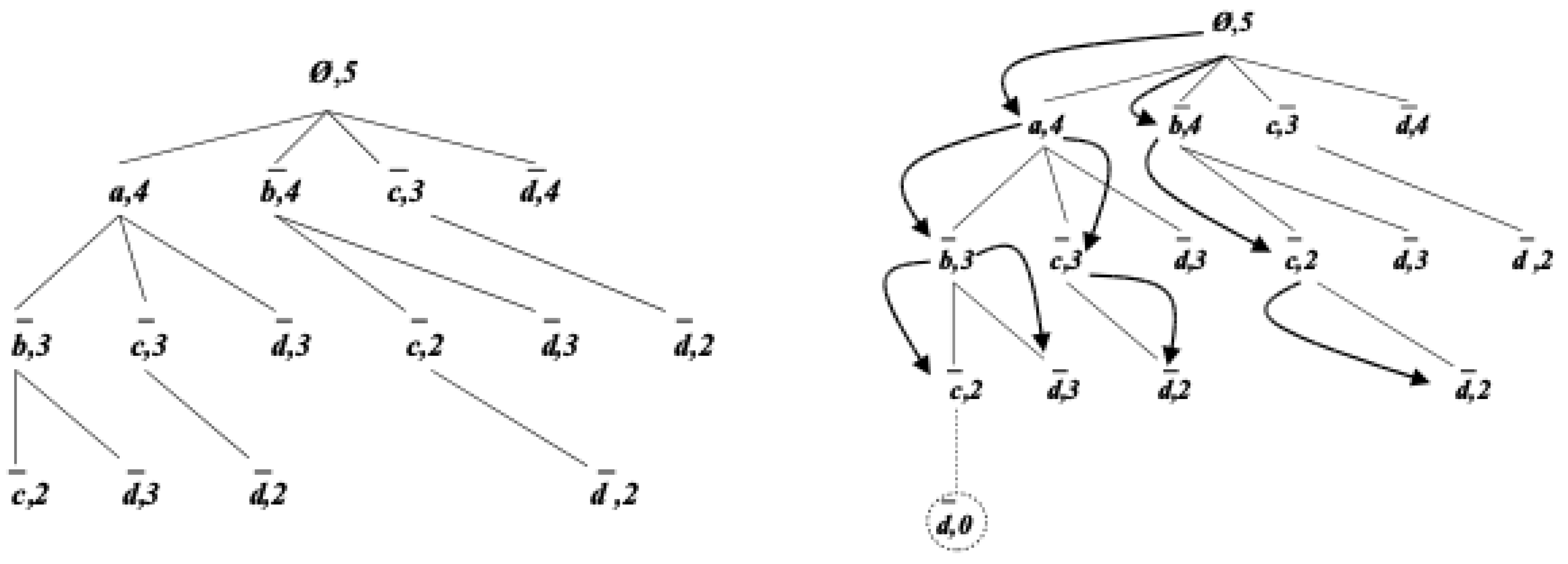
The FasterIE algorithm adopts a bottom-up traversal of the search space. Hence, starting from the empty set, it determines frequent literalsets in a growing manner and it stores them into a prefix tree (aka trie) [24]. Figure 2 (Left) shows a prefix tree that stores all strict subsets of the literalset $a\overline{b}\overline{c}\overline{d}$, which can be extracted from the database $\mathcal{D}$ depicted in Table 1. The prefix tree nodes are ordered according to the lexicographic order on literals (the lexicographic order used is given by $a\prec \dots \prec z\prec \overline{a}\prec \dots \prec \overline{z}$). Each path, starting from the root node of the prefix tree, represents a literalset, where the integer kept in the last node on the path stands for the support of the literalset, e.g., the left-most path from the node labeled “∅, 5” to the node labeled “$\overline{c}$, 2” represents the literalset $a\overline{b}\overline{c}$, whose support value is equal to 2.

In the following, we thoroughly describe the different steps of the FasterIE algorithm, whose pseudo-code is presented by Algorithm 1.

In the following, we describe the main routines invoked by the FasterIE algorithm, namely the Generate-frequent-1-literalsets, the Generate-next-level, and the Partial-Computat ion-Support.

Algorithm 1: FasterIE Algorithm

Data: (database $\mathcal{D}$, minsup)

Results: $\mathcal{FL}$

Begin

1  Set of frequent literalsets $\mathcal{FL}$←∅;

2  $\mathcal{FL}$←Generate-frequent-1-literalsets($\mathcal{D}$);

3      do

4      Set of candidates $\mathcal{CL}$←Generate-next-level($\mathcal{FL}$);

for each literalset L in $\mathcal{CL}$ do

5          Partial-Computation-Support(L, root node $n_{\varnothing }$);

6      Scan $\mathcal{D}$ to compute the support of positive variation of each literalset

in $\mathcal{CL}$;

7      $\mathcal{CL}$←Prune-Infrequent-literalsets( $\mathcal{CL}$, minsup);

8      $\mathcal{FL}$←$\mathcal{FL}$ ∪ $\mathcal{CL}$;

9    while$\mathcal{CL}$ is non empty

return $\mathcal{FL}$;

End

6.1. The Generate-Frequent-1-Literalsets Procedure

The Generate-frequent-1-literalsets procedure scans the transaction database to find out the set of frequent 1-literalsets. To this end, it uses a temporary |$\mathcal{I}$|-sized array, where the ith entry represents the support of the positive literal i. Initially, entries of the array are set to 0. Then, for each scanned transaction T of the database, the support of the literal i is incremented if i is contained in T. Straightforwardly, we can deduce the support of each negative literal $\overline{i}$ from that of its opposite i, thanks to Supp($\overline{i}$) = Supp($\varnothing )-\mathit{Supp}(i$). The procedure creates the root node $n_{\varnothing }$ containing the empty set and its support value equal to $\left|\mathcal{D}\right|$ and its child nodes representing frequent literals with their associated supports.

6.2. The Generate-Next-Level Procedure

During an iteration k, the procedure uses the prefix tree to generate the candidate k-literalsets. For this purpose, Generate-next-level creates for each pair of (k − 1)-literalsets $L1$ and $L2$, sharing the same ($k-2$)-elements in the prefix tree, a candidate child node $n_{L1 \cup L2}$. Furthermore, the procedure leverages the anti-monotonicity property of the support measure, to prune candidate k-literalsets, which have at least one infrequent (k − 1)-subset. Figure 2 (Bottom) illustrates the Generate-next-level procedure at work.

6.3. Computing Supports of the Literalsets

The purpose of this step is to compute the respective supports of candidate literalsets. To this end, we propose to split this phase into two sub-phases as follows:

6.3.1. The Partial-Computation-Support

To compute the support of a candidate k-literalset L, we first call the Partial-Computation-Support procedure, whose pseudo-code is given by Algorithm 2. This procedure only allows computing the value of the subtractive term in Equation (2) (c.f. Theorem 1). To do so, the supports of the subsets of L sharing PosPart$(L)$ are required. It is important to note that these support values were already determined during previous iterations. To this end, Partial-Computation-Support uses an array of size $\left|L\right|$, denoted by Z. The ith entry of Z, denoted by $Z\left[i\right]$, contains the ith literal in L.

Algorithm 2: Partial-Computation-Support Procedure

Data: (literalset L, n)

/* assert: Supp(L) stores the support of the literalset L */

/* assert: Z stores literals of the literalset L */

Begin

1  i := 0;

2  whileZ[i] is not the last positive literal in Ldo

3    n := n→$n_{Z[i]}$;

4    i := i + 1;

5  Supp(L) := 0;

6  Explore(Z, i, n, Supp(L));

End

This procedure traverses the prefix-tree starting from the root node. Two-pointers are used. The first pointer p runs through the elements of Z and is initialized to the first element. The second pointer q runs through the nodes of the prefix-tree, and it is initialized to the root node $n_{\varnothing }$. For a literal $Z\left[i\right]$ referenced by p, Partial-Computation-Support checks whether p is not the last positive literal in L. If so, it runs through the node’s children referenced by q to locate the node with label $Z\left[i\right]$. Otherwise, p is the last positive literal in L, and we begin by retrieving the supports of the literalsets according to Theorem 1, since they share PosPart(L). Indeed, we explore descendants of the node referenced by q, by invoking recursively the Explore procedure, whose pseudo-code is given by Algorithm 3.

Algorithm 3:  Explore Procedure

Data: (Z, n, i, Supp(L))

Begin

1  n := n→$n_{Z\left[i\right]}$;

2  Supp(L) = Supp(L) ± $n.$Supp;

3  for(j := i + 1; j < |L|; j := j + 1)

4   Explore(Z, n, j, Supp(L));

End

In fact, this procedure looks for children nodes of the node referenced by q, whose labels are included in NegPart$(L)$). Then, for each children node $n_c$, the support of L is updated with support of $n_c$ and Explore is recalled. The search process comes to an end whenever any pointer reaches the end of its structures.

Example 4.

In Figure 3, the Partial-Computation-Support procedure is illustrated for the candidate literalset $a\overline{b}\overline{c}\overline{d}$. The arrows indicate the nodes that are summed.

6.3.2. Computation of Supports of Positive Variations

Once the subtractive term of each candidate k-literalset L is computed, the FasterIE algorithm computes the first term which represents the support of PosVar$(L)$, cf. Theorem 1. It is important to note that this computation requires only one scan of the database for the whole set of the candidate k-literalsets.

Finally, after computing supports of the candidate k-literalsets, the algorithm deletes leaves presenting a support value lower than minsup (cf. Algorithm 1, line 8).

6.4. Optimization Issues

It is noteworthy that FasterIE has to make many node visits through the prefix tree to compute the support of a literalset. Consequently, to improve the performance of FasterIE algorithm, we should devise strategies which minimize as far as possible the number of node visits.

• Strategy 1: The first optimization is based on the following observation. As shown before, during partial counting of the support of a candidate literalset, the algorithm explores nodes that have been already visited during the checking subsets step. For example, in Figure 3, the framed nodes were already visited when subsets of $a\overline{b}\overline{c}\overline{d}$ were handled. Thus, combining these two steps would be advantageous.
• Strategy 2: According to Theorem 1, we can remark that some supports needed to compute the support of a literalset L are also required to compute the support of L subsets sharing PosPart$(L)$). For example, we have:

$$\mathit{Supp}(a\overline{c}\overline{d})=-\mathit{Supp}(a)+\mathit{Supp}(a\overline{c})+\mathit{Supp}(a\overline{d})+\mathit{Supp}(acd)$$

(3)

$$\mathit{Supp}(a\overline{b}\overline{c}\overline{d})=\mathit{Supp}(\mathit{a})-\mathit{Supp}(a\overline{b})-\mathit{Supp}(\mathit{a}\overline{\mathit{c}})-\mathit{Supp}(\mathit{a}\overline{\mathit{d}})+\mathit{Supp}(a\overline{b}\overline{c})+\mathit{Supp}(a\overline{b}\overline{d})+\mathit{Supp}(\mathit{a}\overline{\mathit{c}}\overline{\mathit{d}})-\mathit{Supp}(abcd)$$

(4)

Consequently, we can replace terms of Equation (4) shared with Equation (3) by Supp(PosVar$(a\overline{c}\overline{d})$).

$$\mathit{Supp}(a\overline{b}\overline{c}\overline{d})=-\mathit{Supp}(a\overline{b})+\mathit{Supp}(a\overline{b}\overline{c})+\mathit{Supp}(a\overline{b}\overline{d})+\mathit{Supp}(\mathit{acd})-\mathit{Supp}(abcd)$$

(5)

According to Equation (5), we remark that instead of looking for Supp($\mathit{a}$), Supp($\mathit{a}\overline{\mathit{c}}$), Supp($\mathit{a}\overline{\mathit{d}}$), and Supp($\mathit{a}\overline{\mathit{c}}\overline{\mathit{d}}$), we only have to recuperate Supp(PosVar$(a\overline{c}\overline{d})$).

To generalize this example, we propose to further refine the computation support of a literalset L as follows:

Proposition 1.

Let L = $\{i_1$, …, $i_m$, ${\overline{j}}_1$, …, ${\overline{j}}_n\}$ be a literalset.

$\mathit{Supp}$(L) = ${(-1)}^n$ × $\mathit{Supp}$($\{i_1,\dots ,i_m,j_1,\dots ,j_n\}$) + $\mathit{Supp}$($\{i_1,\dots ,i_m,j_2,\dots ,j_n\}$)

$$-\sum _{S\subset \{{\overline{j}}_2,\dots ,{\overline{j}}_n\}}{(-1)}^{|S^{\prime }|}\times \mathit{Supp}(\{i_1,\dots ,i_m,{\overline{j}}_1\}\cup S)$$

with |$S^{\prime }$| = |S| if n is even and |$S^{\prime }$| = |S| + 1 if n is odd.

Proof. 

According to Theorem 1, we have:

Supp($\{i_1,\dots ,i_m,{\overline{j}}_1,\dots ,{\overline{j}}_n\}$) = ${(-1)}^n$ × Supp($\{i_1,\dots ,i_m,j_1,\dots ,j_n\}$)

$$+\sum _{S\subset \{{\overline{j}}_1,\dots ,{\overline{j}}_n\}}{(-1)}^{|S^{\prime }|}\times \mathit{Supp}(\{i_1,\dots ,i_m\}\cup S)$$

Hence,

Supp($\{i_1,\dots ,i_m,{\overline{j}}_1,\dots ,{\overline{j}}_n\}$) = ${(-1)}^n$ × Supp($\{i_1,\dots ,i_m,j_1,\dots ,j_n\}$)

$$+\sum _{S\subseteq \{{\overline{j}}_2,\dots ,{\overline{j}}_n\}}{(-1)}^{|S^{\prime }|}\times \mathit{Supp}(\{i_1,\dots ,i_m\}\cup S){(\mathit{E}}_{\mathit{6}})$$

$$+\sum _{S\subset \{{\overline{j}}_2,\dots ,{\overline{j}}_n\}}{(-1)}^{|S^{\prime }|}\times \mathit{Supp}(\{i_1,\dots ,i_m,{\overline{j}}_1\}\cup S)$$

By applying Theorem 1 for the literalset $\{i_1,\dots ,i_m,{\overline{j}}_2,\dots ,{\overline{j}}_n\}$, we obtain:

Supp($\{i_1,\dots ,i_m,{\overline{j}}_2,\dots ,{\overline{j}}_n\}$) = ${(-1)}^n$ × Supp($\{i_1,\dots ,i_m,j_2,\dots ,j_n\}$)

$$+\sum _{S\subset \{{\overline{j}}_2,\dots ,{\overline{j}}_n\}}{(-1)}^{|S^{\prime }|}\times \mathit{Supp}(\{i_1,\dots ,i_m\}\cup S)$$

Hence,

${(-1)}^n$ × Supp($\{i_1,\dots ,i_m,j_2,\dots ,j_n\}$) = Supp($\{i_1,\dots ,i_m,{\overline{j}}_2,\dots ,{\overline{j}}_n\}$)

$${(\mathit{E}}_{\mathit{7}})+\sum _{S\subset \{{\overline{j}}_2,\dots ,{\overline{j}}_n\}}{(-1)}^{|S^{\prime }|}\times \mathit{Supp}(\{i_1,\dots ,i_m\}\cup S)$$

$$=\sum _{S\subseteq \{{\overline{j}}_2,\dots ,{\overline{j}}_n\}}{(-1)}^{|S^{\prime }|}\times \mathit{Supp}(\{i_1,\dots ,i_m\}\cup S)$$

By replacing (E${}_{\mathit{6}}$) by (E${}_{\mathit{7}}$), we deduce that:

Supp($\{i_1,\dots ,i_m,{\overline{j}}_1,\dots ,{\overline{j}}_n\}$) = ${(-1)}^n$ × Supp($\{i_1,\dots ,i_m,j_1,\dots ,j_n\}$)

+ Supp($\{i_1,\dots ,i_m,j_2,\dots ,j_n\}$)

$$+\sum _{S\subset \{{\overline{j}}_2,\dots ,{\overline{j}}_n\}}{(-1)}^{|S^{\prime }|}\times \mathit{Supp}(\{i_1,\dots ,i_m,{\overline{j}}_1\}\cup S)$$

□

However, it is essential to underscore that we have to store the positive variation of literalsets in its corresponding node.

7. Experimental Evaluation

To assess the performances of the FasterIE algorithm, we carried out experiments considered on benchmark datasets taken from the UCI Machine Learning Database Repository (the datasets, accessed on 7 November 2021, are available at http://www.ics.uci.edu/mlearn/MLRepository.html).

7.1. Assessing Optimizations Benefits

The first series of experiments were performed to compare the first version of FasterIE to the second one, i.e., using the optimizations mentioned above, denoted by FasterIE+. According to Figure 4, we can notice that the optimized version largely outperforms the first version of FasterIE, especially as far as we lower minsup values. For example, for the lowest threshold, FasterIE+ is 32 times, 6 times, 8 times, and 7 times as fast as FasterIE respectively for the Nursery, Monks, Flare, and Zoo datasets. This is can be explained by the fact that both introduced optimizations allow to considerably reduce the number of visited nodes during the step of computing of literalset supports.

7.2. Performance of the FasterIE Algorithm

In the following, we evaluate the FasterIE algorithm in its optimized version. To this end, two different series of experiments were held as follows:

• The first series of experiments: This series consists of comparing FasterIE versus the naive brute-force approach. To this end, we first extended the tested databases. Then, we used the efficient Bodon implementation [25] of the Apriori algorithm to extract frequent literalsets (this implementation, accessed on 4 September 2021, is available at http://fimi.cs.helsinki.fi/). According to Figure 5, we notice that FasterIE largely outperforms Apriori. Indeed, our algorithm performs 10–72 times faster than its competitor Apriori. A takeaway message from this first series of experiments is that we can observe that the brute-force naive approach is, expectantly, the furthest from being scalable.
• The second series of experiments: In this series, we compare the FasterIE algorithm versus its competitors, i.e., to those extracting frequent literalsets from the original dataset. In [23], Calders and Goethals presented three methods for computing the support of a literalset (these approaches were used to extract the non-derivable itemsets [26]). we leveraged these approaches to implement three algorithms, denoted by BruteForceIE, CombinedIE, and QIE in order to extract frequent literalsets. As aforementioned, these methods have to access the dataset further to compute the required supports of several infrequent positive itemsets. It is worthy of mention to note that we omit the experimental results of QIE because it is a very time-consuming algorithm. For example, for the Zoo database, it takes more than eight hours for a minsup value equal to $60\%$. A glance to Figure 5, we notice that FasterIE algorithm outperforms BruteForceIE by many orders of magnitude. This is explained by the fact that BruteForceIE performs a high number of database scans to determine the respective literal supports. Indeed, the algorithm has to scan the database for each support computation. Consequently, the more significant negative literaset part is, the slower the algorithm becomes. This conclusion is reasonably expected since the number of terms of Equation (1) exponentially grows with the number of negative literals. As we have already underscored, the larger the negative literaset part, the trickier and more challenging the literaset support computation. Our approach comes into play since we put forward that according to Proposition 1, we underscore that some supports needed to compute the support of a literalset L are also be reused to compute the support of L subsets sharing part. Thus, we are rewriting in terms of its support, and we are decreasing the length of negative literaset part. By and large, FasterIE algorithm sharply outperforms CombinedIE, which on his turn outperforms the BruteForceIE algorithm. Indeed, the CombinedIE algorithm reduces the I/O cost by storing all transactions in a trie-like data structure [27].

8. Conclusions

Generalized association rules mining is a highly relevant yet challenging problem in data mining that has caught many researchers’ interest. Indeed, when negative items are considered, the length of the transactions increases. Thus, the standard algorithms of data mining and especially the step of computing the supports of itemsets with negation would break down.

This paper focuses on a critical step of generalized association rules mining, namely extracting frequent literalsets. Indeed, this step constitutes the basis of the mining process of generalized association rules. To this end, we proposed a new algorithm, called FasterIE, for extracting frequent literalsets. In addition, we devise an efficient method that overcomes the problem of computing the support of literalsets. Experimental results show the proposed approach’s efficiency compared to the existing algorithms.

The number of generalized association rules can be overwhelming. Thus, it is nearly impossible for the end-users to comprehend or validate many such rules. In this line, we are planning to tackle the pay heed to these thriving challenges:

• Mining generic bases of top-K of generalized association rules [28]: The massive number of association rules drawn from– even reasonably sized datasets–bootstrapped the development of more acute techniques or methods to reduce the size of the reported rule sets. The sought-after goal would be to define“ irreducible” nuclei of generalized association rule subset. From such a generic basis of generalized association rules, it is possible to infer all association rules commonly via an adequate axiomatic system. We also consider exploring the benefit of applying this newly defined generic basis for the regulation of Pregnancy Associated Breast Cancer Gene Expressions [29],
• A conceptual coverage composed of generalized literalsets [6,30]: This issue explores the thriving opportunity to define a generalized conceptual coverage by generalized intent and extent parts. Would it be better, or more convenient, to describe some properties by the absence of the other ones?
• Identification of biclusters in gene expression data [31]: Indeed, biclusters can be of positive or negative correlations. A negative correlations bicluster is a bicluster where the expression values of some genes tend to be the complete opposite of the other genes, i.e., given two genes $G_1$ and $G_2$, under the same condition C, if both $G_1$ and $G_2$ are affected by C. At the same time, $G_1$ goes up, and $G_2$ goes down, we can note that $G_1$ and $G_2$ have a negative correlation pattern.

References

- Solanki, S.K.; Patel, J.T. A Survey on Association Rule Mining. In Proceedings of the Fifth International Conference on Advanced Computing Communication Technologies, Haryana, India, 21–22 February 2015; pp. 212–216. [Google Scholar]
- Sharma, R.; Kaushik, M.; Peious, S.A.; Bazin, A.; Shah, S.A.I.F., Jr.; Ben Yahia, S.; Draheim, D. A Novel Framework for Unification of Association Rule Mining, Online Analytical Processing and Statistical Reasoning. IEEE Access 2022, 10, 12792–12813. [Google Scholar] [CrossRef]
- Fister, I.I.F., Jr. Association Rules over Time. In Frontiers in Nature-Inspired Industrial Optimization; Springer: Singapore, 2022; pp. 1–16. [Google Scholar] [CrossRef]
- Fournier-Viger, P.; Li, J.; Lin, J.C.; Truong Chi, T.; Uday Kiran, R. Mining cost-effective patterns in event logs. Knowl.-Based Syst. 2020, 191, 105241. [Google Scholar] [CrossRef]
- Mouakher, A.; Ben Yahia, S. Anthropocentric Visualisation of Optimal Cover of Association Rules. In Proceedings of the 7th International Conference on Concept Lattices and Their Applications, Sevilla, Spain, 19–21 October 2010; Volume 672, pp. 211–222. [Google Scholar]
- Mouakher, A.; Ben Yahia, S. QualityCover: Efficient binary relation coverage guided by induced knowledge quality. Inf. Sci. 2016, 355–356, 58–73. [Google Scholar] [CrossRef]
- Mouakher, A.; Ragobert, A.; Gerin, S.; Ko, A. Conceptual Coverage Driven by Essential Concepts: A Formal Concept Analysis Approach. Mathematics 2021, 9, 2694. [Google Scholar] [CrossRef]
- Shahin, M.; Arakkal Peious, S.; Sharma, R.; Kaushik, M.; Ben Yahia, S.; Shah, S.A.; Draheim, D. Big data analytics in association rule mining: A systematic literature review. In Proceedings of the 3rd International Conference on Big Data Engineering and Technology (BDET), Singapore, 16–18 January 2021; pp. 40–49. [Google Scholar]
- Sharmila, S.; Vijayarani, S. Association rule mining using fuzzy logic and whale optimization algorithm. Soft Comput. 2021, 25, 1431–1446. [Google Scholar] [CrossRef]
- Bagui, S.; Probal, D. Mining Positive and Negative Association Rules in Hadoop’s MapReduce Environment. In Proceedings of the ACMSE 2018 Conference, ACMSE’18, Richmond, KY, USA, 29–31 March 2018; Association for Computing Machinery: New York, NY, USA, 2018. [Google Scholar] [CrossRef]
- Wu, X.; Zhang, C.; Zhang, S. Efficient mining of both positive and negative association rules. ACM Trans. Inf. Syst. 2004, 22, 381–405. [Google Scholar] [CrossRef]
- Mahmood, S.; Shahbaz, M.; Guergachi, A. Negative and Positive Association Rules Mining from Text Using Frequent and Infrequent Itemsets. Sci. World J. 2014, 2014, 973750. [Google Scholar] [CrossRef] [PubMed]
- Agrawal, R.; Imielinski, T.; Swami, A. Mining association rules between sets of items in large databases. In Proceedings of the ACM-SIGMOD International Conference on Management of Data (SIGMOD 1993), Washington, DC, USA, 26–28 May 1993; pp. 207–216. [Google Scholar]
- Amir, A.; Feldman, R.; Kashi, R. A new versatile method for association generation. In Proceedings of the 1st European Symposium on Data Mining and Knowledge Discovery (PKDD 1997), Trondheim, Norway, 24–27 June 1997; pp. 221–231. [Google Scholar]
- Savasere, A.; Omiecinski, E.; Navathe, S. Mining for strong negative associations in a large database of customer transactions. In Proceedings of the 14th International Conference Data Engineering 1998 (ICDE 1998), Orlando, FL, USA, 23–27 February 1998; pp. 494–502. [Google Scholar]
- Morzy, M. Efficient mining of dissociation rules. In Proceedings of the 8th International Conference on Data Warehousing and Knowledge Discovery (DaWak 2006), Krakow, Poland, 4–8 September 2006. [Google Scholar]
- Piatetsky-Shapiro, G. Discovery, Analysis, and Presentation of Strong Rules. In Knowledge Discovery in Databases; Piatetsky-Shapiro, G., Frawley, W.J., Eds.; AAAI/MIT Press: Cambridge, MA, USA, 1991; pp. 229–248. [Google Scholar]
- Antonie, M.; Zaïane, O. Mining positive and negative association rules: An approach for confined rules. In Proceedings of the 8th European Conference on Principles and Practice of Knowledge Discovery in Databases (PKDD 2004), Pisa, Italy, 20–24 September 2004; pp. 27–38. [Google Scholar]
- Tan, P.; Kumar, V. Interestigness measures for association patterns: A perspective. In Proceedings of the International Workshop on Postprocessing in Machine Learning and Data Mining, Boston, MA, USA, 20–23 August 2000. [Google Scholar]
- Cornelis, C.; Yan, P.; Zhang, X.; Chen, G. Mining positive and negative association rules from large databases. In Proceedings of the International Conference on Cybernetics and Intelligent Systems (CIS 2006), Bangkok, Thailand, 19–21 November 2006; pp. 613–618. [Google Scholar]
- Boulicaut, J.F.; Bykowski, A.; Jeudy, B. Towards the tractable discovery of association rules with negations. In Proceedings of the 4th International Conference on Flexible Query Answering Systems (FQAS 2000), Warsaw, Poland, 25–28 October 2000; pp. 425–434. [Google Scholar]
- Knuth, D.E. Fundamental Algorithms; Addison-Wesley: Reading, MA, USA, 1997. [Google Scholar]
- Calders, T.; Goethals, B. Quick Inclusion-Exclusion. In Proceedings of the 4th International Workshop Knowledge Discovery in Inductive Databases (KDID 2005), Porto, Portugal, 3 October 2005. [Google Scholar]
- Fredkin, E. Trie memory. Commun. ACM 1960, 3, 490–499. [Google Scholar] [CrossRef]
- Bodon, F. A fast Apriori implementation. In Proceedings of the IEEE ICDM Workshop on Frequent Itemset Mining Implementations (FIMI 2003), Melbourne, FL, USA, 19 December 2003. [Google Scholar]
- Calders, T.; Goethals, B. Non-derivable itemset mining. Data Min. Knowl. Discov. 2007, 14, 171–206. [Google Scholar] [CrossRef] [Green Version]
- Borgelt, C.; Krus, R. Induction of association rules: Apriori implementation. In Proceedings of the 15th Conference on Computational Statistics (COMPSTAT 2002), Berlin, Germany, 24–28 August 2002; pp. 395–400. [Google Scholar]
- Ben Yahia, S.; Gasmi, G.; Mephu Nguifo, E. A new generic basis of “factual” and “implicative” association rules. Intell. Data Anal. 2009, 13, 633–656. [Google Scholar] [CrossRef]
- Bouasker, S.; Inoubli, W.; Ben Yahia, S.; Diallo, G. Pregnancy Associated Breast Cancer Gene Expressions: New Insights on Their Regulation Based on Rare Correlated Patterns. IEEE ACM Trans. Comput. Biol. Bioinform. 2021, 18, 1035–1048. [Google Scholar] [CrossRef] [PubMed]
- Mouakher, A.; Ben Yahia, S. On the efficient stability computation for the selection of interesting formal concepts. Inf. Sci. 2019, 472, 15–34. [Google Scholar] [CrossRef]
- Houari, A.; Ayadi, W.; Ben Yahia, S. A new FCA-based method for identifying biclusters in gene expression data. Int. J. Mach. Learn. Cybern. 2018, 9, 1879–1893. [Google Scholar] [CrossRef]