Measurement and Analysis of High Frequency Assert Volatility Based on Functional Data Analysis

Abstract

Information and communication technology have enabled the collection of high-frequency financial asset time series data. However, the high spatial and temporal resolution nature of these data makes it challenging to compare financial asset characteristics patterns and identify the risk. To address this challenge, a method for realized volatility calculation based on the functional data analysis (FDA) method is proposed. A time–price functional curve is constructed by the functional data analysis method to calculate the realized volatility as the curvature integral of the time–price functional curve. This method could effectively eliminate the interference of market microstructure noise, which could not only allow capital asset price to be decomposed into a continuous term and a noise term by asymptotic convergence, but also could decouple the noise from the discrete-time series. Additionally, it could obtain the value of volatility at any given time, which is no concern about correlations between repeated, mixed frequencies and unequal intervals sampling problems and relaxes the structural constraints and distribution setting of data acquisition. To demonstrate our methods, we analyze a per-second level financial asset dataset. Additionally, sensitivity analysis on the selection of the no equally spaced sample is conducted, and we further add noise to ensure the robustness of our methods and discuss their implications in practice, especially being conducive to more micro analysis of the volatility of the financial market and understanding the rapidly changing changes.

1. Introduction

In recent years, with the rapid and convenient acquisition of high-frequency data of asset returns, scholars and investors have given an increasing amount of attention to volatility modeling [1,2]. ARCH class model, SV class model, and realized volatility class model are used to calculate volatility [3,4,5]. However, these three class models characterize volatility indirectly through rate of return and cannot depict dynamic changes at the intraday level. In particular, modeling intraday volatility usually uses continuous time stochastic process methods [6,7,8], which assume that volatility is generated by a potentially unknown diffusion process. However, these methods are unable to describe and characterize the long memory and periodicity intraday fluctuations. A commonality in these methods depends on the discrete-time points at which the measurements are taken, which are often called point-based realized volatility calculation models [9]. When the data sampling frequency is high enough and the sampled data do not cause micro-market interference, these methods of calculating realized volatility are in theory consistent estimators of true volatility.

With the development of data acquisition technology, the frequency of financial data acquisition is getting higher and higher. As the data sampling frequency increases, the interference of market microstructure noise on data becomes more and more obvious, such as bid–ask spread, infrequent trading, and so on [10,11,12]. If each sample is noisy, point-based realized volatility calculation models are challenged. For example, the sum of returns squares extremely depend on two consecutive price sampling points from $t-1$ to t, where t denotes a time variable. The sampling points themselves are biased and different sampling points may lead to different calculations [13]. Second, high-frequency data have a long memory, which indicates that past shocks persist into the future and have a big impact on the expected future [14,15,16]. In this framework, systemic changes in trading should be considered.From a temporal evolution perspective, if the price is considered and analyzed as discrete time series, the underlying stochastic process that generates these observations cannot be ascertained in terms of statistical analysis. That is to say, the asset price shifting from a time t-1 to t is not independent from current characteristics but should be considered systemic changes. Therefore, faced with these challenges, it is necessary to analyze the high-frequency data’s volatility modeling.

A method about the curve-based realized volatility calculation model is proposed. Discrete time series can be a sampling set of curves, which can be observed over time [17,18]. On the one side, a functional data analysis method could often be used to extract additional information from discrete time series, such as their derivatives to measure the velocity and acceleration of the price curve [19]. On the other side, applying the functional data analysis method could help identify the repeated patterns of price changes in financial markets [20,21]. High-frequency data contain a rich source of information, which provides opportunities to analyze the dynamic changes of short time intervals. However, these studies do not consider decoupling noise from discrete time series. The price is assumed to follow the Brownian semimartingale process, and the integral volatility can be estimated by the realized volatility [22]. Therefore, firstly, this study constructs a time–price functional curve on the basis of discrete observations by the functional data analysis method through the Bernstein basis function. Secondly, referring to the theory of differential geometry, this study takes the curvature integral of the time–price functional curve as the realized volatility of high-frequency data in a certain period of time, which is called functional volatility (FV). In addition, the period of time could be set arbitrarily, so we can calculate the realized volatility at any time scale. Even when the time scale is small enough, instantaneous realized volatility could be estimated.

Different from point-based realized volatility calculation methods, the curve-based realized volatility calculation method has three advantages. First, the curve-based realized volatility calculation method could obtain the information about the sampling time point from t-1 and t, where t denotes a time variable. The point-based realized volatility calculation method ignores the capital asset price’s underlying dynamic shifts from one time point to the next. For example, if two adjacent time points have equal price, the return will be zero. However, the shift from one time point to the next time point comprises much information about price changes. Second, the curve-based realized volatility calculation method could effectively eliminate the interference of market microstructure noise on data. The functional data analysis method allows capital asset price to be decomposed into a continuous term and a noise term by asymptotic convergence, which could decouple the noise from the discrete-time series. Third, the curve-based realized volatility calculation method treats the whole curve as a single entity and there is also no concern about correlations between repeated, mixed frequencies and unequal intervals sampling problems [23]. Point-based realized volatility calculation methods are limited by the correlation of repeated samples, the sampling process for irregular data. The functional data analysis method relaxes the structural constraints and distribution setting of data acquisition, which represents a change in framework towards the handling of discrete time series.

The remainder of this study is as follows: Section 2 is the Methods. The Simulation experiments are described in Section 3. Conclusions and future work are described in Section 4.

2. Methods

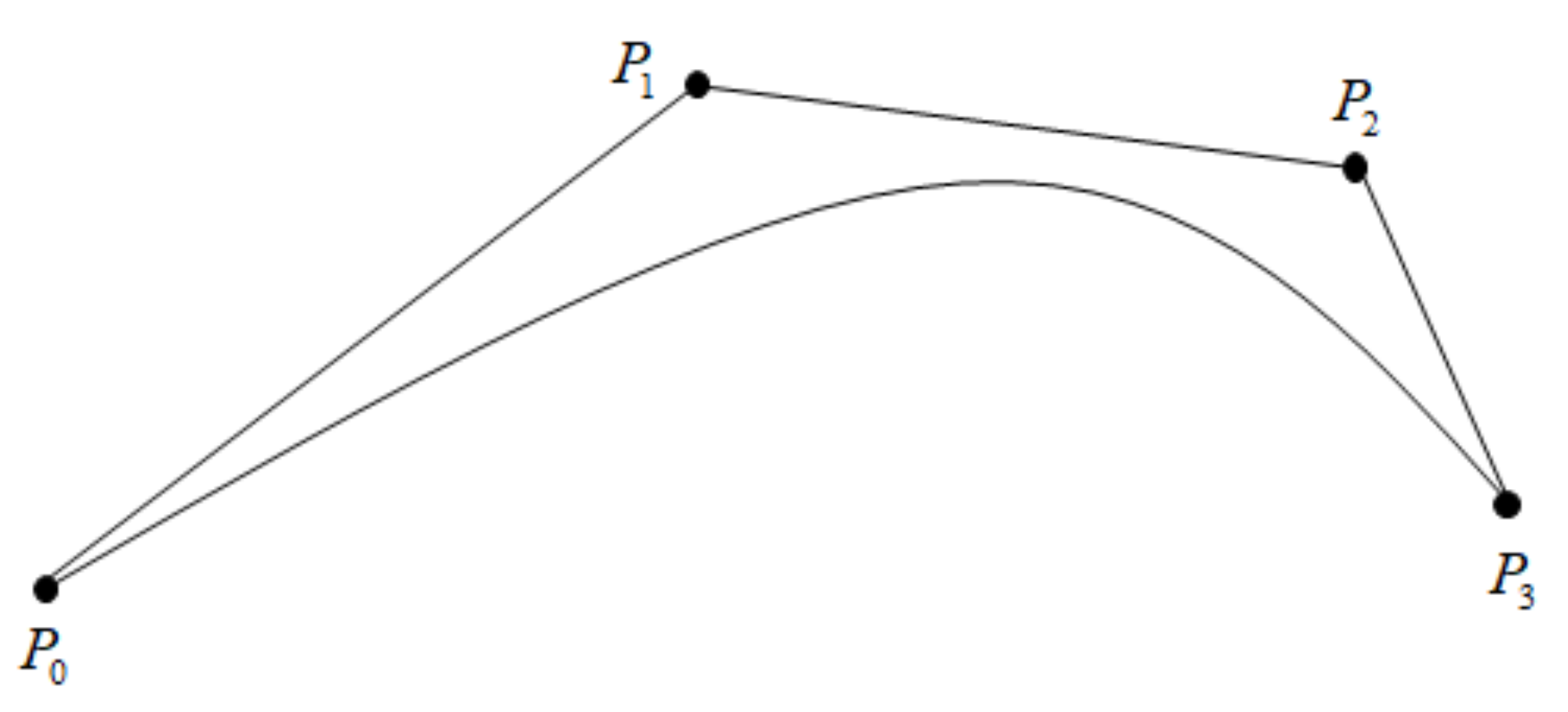
2.1. Determination of Basis Function

Functional data analysis (FDA) takes the functional data as the research object, regarding the observed data as a whole [24]. Consider a one-dimensional functional data $X_1\left(t\right),X_2\left(t\right),\dots ,X_n\left(t\right)$, which is an implementation of a stochastic process $X_t$ on a closed interval $\mathcal{F}$. From the dimension of time t, functional data are a kind of infinite-dimensional data [25]. In reality, it is difficult to obtain the curve with complete observation and without measurement error. Therefore, we first assume that

$$W_{ij}=X_i\left(T_{ij}\right)+U_{ij},T_{ij}\in \mathcal{F},1⩽i⩽n,1⩽j⩽M_i$$

(1)

where $U_{ij}$ is the independent and identically distributed observation error and is independent of $X_i$, satisfies $\mathrm{E}\left(U_{ij}\right)=0,\mathrm{E}\left(U_{ij}^2\right)={\sigma }_u^2$. The actual observation data are $\left(T_{ij},W_{ij}\right)$, $i=1,2,\dots ,n;j=1,2,\dots ,M_i$.

Due to the infinite dimension of functional data, it is significant to reduce the dimension. The common method is to expand the functional data using a set of bases. In more detail, suppose that ${\varphi }_1\left(t\right),{\varphi }_2\left(t\right),\dots$ is a set of orthogonal bases defined on a closed interval $\mathcal{I}$:

$$X\left(t\right)=\sum _{k=1}^{\infty }{\xi }_k{\varphi }_k\left(t\right)$$

(2)

where ${\xi }_k={\int }_{\mathcal{I}}X\left(t\right){\varphi }_k\left(t\right)\mathrm{d}t$ is the projection of $X_t$ on ${\varphi }_k\left(t\right)$. In practice, we need to truncate the number of expansions, that is, $X\left(t\right)\approx {\sum }_{k=1}^K{\xi }_k{\varphi }_k\left(t\right)$. In this way, the infinite-dimensional functional data $X_t$ are approximated to the sum of the expansions of finite terms. The information contained in infinite-dimensional function data can be expressed by a finite-dimensional vector ${\left({\xi }_1,{\xi }_2,\dots ,{\xi }_K\right)}^{\top }$ to achieve the purpose of dimension reduction.

Let the time series data be $Y_i,i=0,1,\cdots ,n$, and the fitting model can be constructed as follows:

$$Y\left(t\right)=\sum _{j=0}^m{\beta }_j{\phi }_j\left(t\right)+\epsilon \left(t\right),0\le t\le 1,m<n$$

(3)

where ${\phi }_j\left(t\right),j=0,1,\cdots ,m$ are a set of basis functions; ${\beta }_j,j=0,1,\cdots ,m$ denote the coefficient vector to be determined; ${\epsilon }_j\left(t\right),j=0,1,\cdots ,m$ represent the noise.

The time series $Y_t$ given here is the result of parameterization of the original time series data $Y_i$$(i=0,1,\cdots ,n)$. The determined parameters are divided into ${\Delta }_t:t_0<t_1<\cdots <t_n$. In this way, we are faced with the problem of which basis function should be chosen. First of all, it should be noted that polynomial functions can meet the requirements of mining useful information from complex data, and it is easy to calculate the function value and the derivative value of each order to realize visualization.

All the m-degree polynomials constitute the m-degree polynomial space, and any group of M + 1 linearly independent polynomials in a polynomial space of degree M can be regarded as a group of bases [26]. To better reflect the regularity of complex data, the number of data transformation peaks and valleys is described by m. Through computer input and interactive modification of the fitting curve, we can achieve the goal of description.

The same curve can be represented by different polynomial basis functions, with different properties. Power polynomials $t^j,j=1,\cdots ,m$ reflect the simplest polynomial basis [27]. The curve fitted by the power base has the advantages of simple form and easy calculation. However, the geometric mean of the coefficient vector in the power-based polynomial curve equation is not obvious. In addition, when the order is large, the coefficient matrix is ill-conditioned due to the system of linear equations that must be solved [28]. Lagrange basis function $L_j\left(t\right)={\prod }_{j\ne i=0}^m\frac{\left(t-t_i\right)}{\left(t_j-t_i\right)}$, $j=0,1,\cdots ,m$ is normative and has obvious regularity [29]. However, its derivation is complicated, and all data points need to be recalculated every time data are added. That is not suitable for the requirements of data mining. Fourier basis $e^{i\omega t}$ can reveal the internal relationship between time and spectrum. However, when using Fourier transform, we need to use all the time-domain information of the signal, which lacks the time-domain positioning function [30]. Considering the characteristics of human–computer interaction and data mining, we select the Bernstein basis function in this paper. As a basis function, Bernstein polynomials are classical Bézier curves and become the foundation to develop complex curves and surfaces. It has many excellent properties, such as normalization, symmetry, recurrence, segmentation and control hull [31]. Therefore, we select the Bernstein basis function in this paper. The model fitted by Bernstein basis function is

$$Y\left(t\right)=\sum _{j=0}^m{\beta }_j{B}_{j,m}\left(t\right)+\epsilon \left(t\right),0\le t\le 1$$

(4)

Here, ${\beta }_j,j=0,1,\cdots ,m$ denotes the coefficient vector, which is called the control point of fitting curve. Basis function

$$B_{j,m}\left(t\right)=C_m^j{t}^j{(1-t)}^{m-j},0\le t\le 1,j=0,1,\cdots ,m$$

(5)

is known as the Bernstein basis function.

Besides the good properties of normalization, symmetry, recurrence and segmentation, the Bernstein function also has a convex–hull property [32]. The convex hull of a point set is defined as the set of all convex combinations formed by the elements of the point set. The convex hull property of the fitting curve with the Bernstein basis function means that the curve always lies in the convex hull of its control vertex (see Figure 1).

2.2. Bernstein Basis Function Modeling

Consider a time series as $Y\left(t\right)$, $0\le t\le 1$. Let mth-degree Bernstein polynomials be as basis functions [31]

$$B_{j,m}\left(t\right)=C_m^j{t}^j{(1-t)}^{m-j},0\le t\le 1,j=0,1,\cdots ,m$$

(6)

Construct the actual model

$$Y\left(t\right)=\sum _{j=0}^m{\beta }_j{B}_{j,m}\left(t\right)+\epsilon \left(t\right)$$

(7)

Fitting the time series data points, the sample regression equation is

$$\widehat{Y}\left(t\right)=\sum _{j=0}^m{\widehat{\beta }}_j{B}_{j,m}\left(t\right),0\le t\le 1$$

(8)

Here, the parameter estimation of ${\beta }_j$ is denoted by ${\widehat{\beta }}_j$. Therefore, the model based on Bernstein basis function is

$$Y\left(t\right)=\sum _{j=0}^m{\widehat{\beta }}_j{B}_{j,m}\left(t\right)+e\left(t\right)$$

(9)

where ${\widehat{\beta }}_j,j=0,1,\cdots ,m$ is the estimator of the control vertex. $B_{j,m}\left(t\right)$ denotes the Bernstein basis function. $e\left(t\right)$ expresses the error term, which is $e\left(t\right)=Y\left(t\right)-\widehat{Y}\left(t\right)$. We can further use the properties of the constructed curve to analyze the development law of the studied phenomenon.

It is noteworthy that $\widehat{Y}\left(t\right)$ is the value of fitting data point $Y\left(t\right)$ on the curve (Equation (8)). The actual value obtained after the interference adjustment parameter is $Y\left(t\right)$ in Equation (9). Moreover, stochastic variable $\epsilon \left(t\right)$ represents an error, including data measurement error and random error. Suppose $\epsilon \left(t\right)\sim N\left(0,{\sigma }^2\right)$, and $cov\left[\epsilon \left(t_1\right),\epsilon \left(t_2\right)\right]=0$ for $t_1\ne t_2$.

In this paper, the least-square method is utilized to estimate the control points ${\beta }_j,j=0,1,\cdots ,m$. The time-series data $Y_i$, $i=0,1,\cdots ,n$ are first parameterized. Let ${\tau }_i$ be the indexes corresponding to $Y_i$, $i=0,1,\cdots ,n$, ${\tau }_i\ge 0$.

By normalizing the parameterization results of the above, the normalized parameterization results are generated:

$$t_i=\frac{{\tau }_i}{max\left({\tau }_i\right)},i=0,1,\cdots ,n$$

(10)

In the measurement of high-frequency asset volatility, n is the number of samples per day. Then, the fitted asset price curve can be determined by the least square approach. Let the fitted curve be

$$\widehat{Y}\left(t_i\right)=\sum _{j=0}^m{\widehat{\beta }}_j{B}_{j,m}\left(t_i\right),i=0,1,\cdots ,n$$

(11)

The sample model is

$$Y\left(t_i\right)=\sum _{j=0}^m{\widehat{\beta }}_j{B}_{j,m}\left(t_i\right)+e\left(t_i\right)$$

(12)

Calculate the control point to minimize the following formula:

$$E=\sum _{i=0}^n{\left(Y\left(t_i\right)-\widehat{Y}\left(t_i\right)\right)}^2$$

(13)

That is,

$$E\left({\widehat{\beta }}_0,{\widehat{\beta }}_1,\cdots ,{\widehat{\beta }}_m\right)=\sum _{i=0}^n{\left(Y\left(t_i\right)-\sum _{j=0}^m{\widehat{\beta }}_j{B}_{j,m}\left(t_i\right)\right)}^2$$

(14)

According to the least square method, the control vertex can be obtained

$$\left[\begin{array}{c}{\widehat{\beta }}_0\\ {\widehat{\beta }}_1\\ ⋮\\ {\widehat{\beta }}_m\end{array}\right]={\left({\Phi }^T\Phi \right)}^{-1}{\Phi }^T\left[\begin{array}{c}Y\left(t_0\right)\\ Y\left(t_1\right)\\ ⋮\\ Y\left(t_n\right)\end{array}\right]$$

(15)

where

$$\Phi =\left[\begin{array}{cccc}{B}_{0,m}\left(t_0\right)& B_{1,m}\left(t_0\right)& \cdots & B_{m,m}\left(t_0\right)\\ B_{0,m}\left(t_1\right)& B_{1,m}\left(t_1\right)& \cdots & B_{m,m}\left(t_1\right)\\ ⋮& \dots & \ddots & \dots \\ B_{0,m}\left(t_n\right)& B_{1,m}\left(t_n\right)& \cdots & B_{m,m}\left(t_n\right)\end{array}\right]$$

(16)

${\Phi }^T$ is the transpose of $\Phi$.

In this way, $m+1$ control points ${\widehat{\beta }}_0,{\widehat{\beta }}_1,\cdots ,{\widehat{\beta }}_m$ in Equation (8) are estimated. The model requires that the fitting curve must coincide with the beginning and end of the original curve. Therefore, we modify the head and tail control points: ${\widehat{\beta }}_0\to Y\left(t_0\right)$, ${\widehat{\beta }}_m\to Y\left(t_n\right)$ to ensure that the piecewise fitting curve can be successfully spliced to form an overall fitting curve, which can represent the whole data samples.

Then, we can obtain the fitting curve

$$\widehat{Y}\left(t\right)=\sum _{j=0}^m{\widehat{\beta }}_j{B}_{j,m}\left(t\right)0\le t\le 1$$

(17)

As for our model, the only parameter to be determined is m, which is finally optimal by the minimum generalized cross-validation criterion (GCV):

$$GCV\left(m\right)=\frac{{\sum }_{i=1}^N{\left(Y\left(t\right)-{\sum }_{j=0}^m{\widehat{\beta }}_j{\beta }_{j,m}\left(t_i\right)\right)}^2}{{(1-M\left(m\right)/N)}^2}$$

(18)

where $M\left(m\right)$ denotes the number of effective parameters in the model, and N is the number of actual observation samples.

2.3. Volatility Measurement

Intuitively, after constructing the function curve of coarse high-frequency data. It is more natural to quantify the volatility through the characteristics of the function than to measure the realized volatility. As a result, we can naturally measure asset volatility by measuring the curve fluctuation degree of the asset curve.

The curvature of the function can be used to determine the degree of volatility of the measurement curve. A curve’s curvature is the rotation rate of the tangent direction angle of a point on this curve to the arc length. It is defined by the differential and represents the curve’s bending at a certain point. The greater the curvature, the greater the degree of curve bending, that is, the greater the degree of fluctuation [33].

Let the constructed asset fluctuation curve equation be $y=f\left(t\right)$, which contains the second derivative. The curvature of a function curve at point M is defined as

$$K=\frac{\left|y^{″}\right|}{{\left(1+y^{\prime 2}\right)}^{\frac{3}{2}}}$$

(19)

According to Equation (11), we can calculate the first and second derivatives of the asset change curve as follows:

$$y^{\prime }=\frac{\partial \widehat{Y}\left(t\right)}{\partial t}=\sum _{j=0}^m{\widehat{\beta }}_j\left[\frac{tm-j}{t(t-1)}\right]B_{j,m}\left(t\right),$$

(20)

$$\begin{array}{cc}\hfill y^{″}& =\frac{{\partial }^2\widehat{Y}\left(t\right)}{\partial t^2}\hfill \\ \hfill & =\sum _{j=0}^m{\widehat{\beta }}_j\left[\frac{m^2+m}{{(t-1)}^2}+\frac{j^2-j}{t^2{(t-1)}^2}+\frac{2j(1-m)}{t{(t-1)}^2}\right]B_{j,m}\left(t\right),\hfill \end{array}$$

(21)

where $0\le t\le 1$. Based on differential geometry theory, the total curvature of a curve is equal to the integral of curvature:

$$F{V}_t={\int }_{t_j}^{t_{j+1}}\frac{\left|y^{″}\right|}{{\left(1+y^{\prime 2}\right)}^{\frac{3}{2}}}dt$$

(22)

The formula above can characterize the volatility of high-frequency asset fluctuations and then be utilized as a volatility measure, which can be called functional volatility (FV). It is noted that the time interval here can be any period.

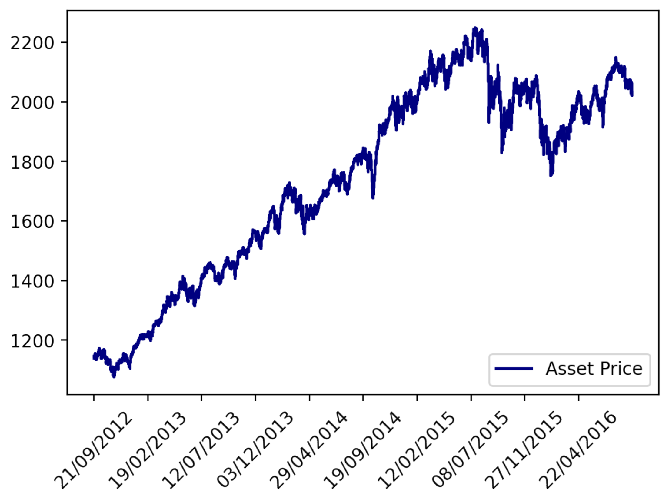
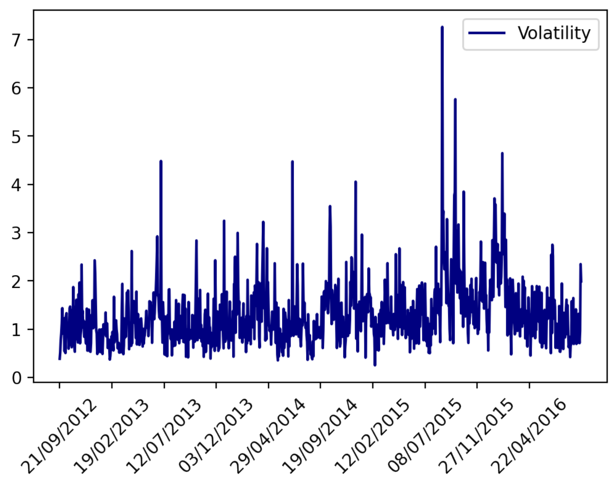
3. Experimental Analysis

To verify the effectiveness of our model, we use real data for empirical analysis and test the unequal spaced sample and noise on a high-frequency asset dataset. Due to a large amount of data, it is impossible to fit well with a low degree polynomial. Therefore, according to the references [34,35], we use 200 data sample points for fitting each time.

The data was obtained from a Thompson Ruter Tick History database (TRTH), which have asset changes per second. In particular, the original data are equidistant. We randomly select 1000 days and use the above model to calculate the daily functional volatility as the gold standard. Figure 2 and Figure 3 illustrate the asset price from 2012 to 2016 years used in this paper and daily volatility measured using complete dataset.

The relative error is chosen as the evaluation criterion in this paper, which can be expressed as

$$\mathrm{Error}=\frac{1}{N}\sum _{i=1}^N\frac{\left|\widehat{F{V}_i}-F{V}_i\right|}{F{V}_i}$$

(23)

where ${\widehat{FV}}_i$, $i=0,1,\cdots ,N$ denotes the the daily volatility obtained by the original dataset, and the $F{V}_i$ indicates the corresponding volatility under simulated conditions.

In detail, we design the following two simulation settings.

• We randomly remove a certain proportion of data from the original daily data, that is, produce non-equidistant high-frequency data. The corresponding proportion is controlled by DropRate.
• We randomly add noise $r*sigma$ to the original data, where r is randomly chosen from 0 to 1. Parameter $sigma$ determines the degree of the added noise.

We presented the maximum (sub), average (avg), and standard (std) error of relative error across 500 replications in

Table 1. Related error results under different drop rates on real data.

DropRate	sub	avg	std
0.1	0.003993	0.000017	0.000192
0.2	0.035771	0.000225	0.001836
0.3	0.115362	0.000767	0.006560

and

Table 2. Relate error results under different sigma on real data.

Sigma	sub	avg	std
0.1	0.032560	0.016152	0.009657
0.2	0.065114	0.031076	0.019011
0.3	0.097928	0.049194	0.029173
0.4	0.130392	0.064272	0.038869

. Results perform the efficiency of our method to address non-equidistant and noisy situations, in which the averaged and related error is less than 10%. In terms of the maximum related errors, the errors are more than 10% when DropRate is equal to 0.3 or the sigma exceeds 0.4.

It is worth noting that we randomly remove the original data in Simulation 1 to produce non-equidistant asset data. At the same time, it also means that we estimate the model with missing data. This also verifies that our model can overcome the case with missing values.

Usually, stock prices are modeled by lognormal distributions [36]. Therefore, we generate 500 days of high-frequency asset price data through lognormal distribution to further verify the effectiveness of our model. Following the above settings, we consider the deviation of the model in the case of random loss of samples and adding noise.

Table 3. Related error results under different drop rates on simulation data.

DropRate	sub	avg	std
0.1	0.001301	0.000209	0.000108
0.2	0.012924	0.000368	0.000861
0.3	0.239079	0.001688	0.012562

and

Table 4. Related error results under different sigma on simulation data.

Sigma	sub	avg	std
0.1	0.000072	0.00004	0.000571
0.2	0.000145	0.000114	0.002248
0.3	0.097928	0.000116	0.001764

demonstrate the relate error results under different drop rate and sigma. Results show that our method has good robustness.

4. Conclusions and Future Work

In recent decades, financial data collection technologies have evolved to allow more intensive sampling of temporal, spatial, and other continuous measurements. At the same time, the available financial data are increasingly complex, such as data being recorded continuously at an interval and data being recorded intermittently at several discrete points in time. Faced with the real situation, this paper proposed the FDA approach to measure the volatility indicators.

The FDA approach represents a change in philosophy on financial time series data processing. Classical multivariate statistical techniques could only obtain information from sampling time points, and they do not take advantage of additional information that could be implied by sampling information between points in time.

The FDA approach indicates that the financial time series data reflect the influence of certain smooth functions that are assumed to underlie the observations. Some additional information could be extracted from the smoothness of underlying functions [37]. For example, topology information, such as derivatives and curvature, could be obtained by curve calculation [38,39]. Therefore, we develop a set of volatility calculation models based on the concept of curvature integration.

Measurement volatility based on the FDA approach could provide a new analytical idea about the financial market for scholars, investors, and policy managers. On the one side, the FDA approach could measure the volatility at any period, especially the instantaneous volatility. This helps us to delve into micro time and explore financial markets. In particular, for policy managers, markets can be monitored in real time. On other hand, the FDA approach represents the financial time series data as a whole curve. Volatility measurement is an example. Time series data are a common form of the finance market. Therefore, in the research on the finance market, it is a good consideration to use the FDA approach or nest the FDA approach in existing methods, such as dimension reduction, clustering, and classification. Possibly, some new, valuable, interesting analyses and findings will emerge.

For future research, this work can be extended to discuss the following three aspects. First, Bernstein polynomials are classical Bézier curves that have become the foundation to develop complex curves and surfaces. Therefore, more complex Bézier polynomials as the basis function of volatility measure deserve to be studied. Second, how to produce the curvature graph for realized volatility curve is also an interesting topic, which can refer to these articles [40]. Finally, as for the measurement method of functional volatility, future research can consider obtaining a better fitting curve through the kernel method and verifying its mathematical properties.

References

1. Weng, F.; Zhang, H.; Yang, C. Volatility forecasting of crude oil futures based on a genetic algorithm regularization online extreme learning machine with a forgetting factor: The role of news during the COVID-19 pandemic. Resour. Policy 2021, 73, 102148. [Google Scholar] [CrossRef] [PubMed]
2. Duttilo, P.; Gattone, S.; Di Battista, T. Volatility modeling: An overview of equity markets in the euro area during COVID-19 Pandemic. Mathematics 2021, 9, 1212. [Google Scholar] [CrossRef]
3. Andersen, T.; Bollerslev, T.; Diebold, F.; Labys, P. The distribution of realized exchange rate volatility. J. Am. Stat. Assoc. 2001, 96, 42–55. [Google Scholar] [CrossRef]
4. Bollerslev, T. Generalized autoregressive conditional heteroskedasticity. J. Econom. 1986, 31, 307–327. [Google Scholar] [CrossRef] [Green Version]
5. Hansen, P.; Huang, Z.; Shek, H. Realized GARCH: A joint model for returns and realized measures of volatility. J. Appl. Econom. 2012, 27, 877–906. [Google Scholar] [CrossRef]
6. Poon, S.; Granger, C. Practical issues in forecasting volatility. Financ. Anal. J. 2005, 61, 45–56. [Google Scholar] [CrossRef] [Green Version]
7. Andersen, T.; Bollerslev, T.; Diebold, F. Parametric and nonparametric volatility measurement. In Handbook of Financial Econometrics: Tools and Techniques; North-Holland: Chicago, IL, USA, 2010; pp. 67–137. [Google Scholar]
8. Hurvich, C.; Moulines, E.; Soulier, P. Estimating long memory in volatility. Econometrica 2005, 73, 1283–1328. [Google Scholar] [CrossRef] [Green Version]
9. Liu, C.; Maheu, J. Are there structural breaks in realized volatility? J. Financ. Econom. 2008, 6, 326–360. [Google Scholar] [CrossRef]
10. Bandi, F.M.; Russell, J.R. Separating microstructure noise from volatility. J. Financ. Econ. 2006, 79, 655–692. [Google Scholar] [CrossRef]
11. Hansen, P.; Lunde, A. Realized variance and market microstructure noise. J. Bus. Econ. Stat. 2006, 24, 127–161. [Google Scholar] [CrossRef]
12. Zhang, L.; Mykland, P.A.; Aït-Sahalia, Y. A tale of two time scales: Determining integrated volatility with noisy high-frequency data. J. Am. Stat. Assoc. 2005, 100, 1394–1411. [Google Scholar] [CrossRef]
13. Duong, D.; Swanson, N. Empirical evidence on the importance of aggregation, asymmetry, and jumps for volatility prediction. J. Econom. 2015, 187, 606–621. [Google Scholar] [CrossRef] [Green Version]
14. Breidt, F.; Crato, N.; Delima, P. The detection and estimation of long memory in stochastic volatility. J. Econom. 1998, 83, 325–348. [Google Scholar] [CrossRef] [Green Version]
15. Baillie, R.; Cecen, A.; Han, Y. High frequency Deutsche Mark-US Dollar returns: FIGARCH representations and non linearities. Multinatl. Financ. J. 2000, 4, 247–267. [Google Scholar] [CrossRef]
16. Granger, C. Long memory relationships and the aggregation of dynamic models. J. Econom. 1980, 14, 227–238. [Google Scholar] [CrossRef]
17. Alvarez, A.; Panloup, F.; Pontier, M.; Savy, N. Estimation of the instantaneous volatility. Stat. Inference Stoch. Process. 2012, 15, 27–59. [Google Scholar] [CrossRef] [Green Version]
18. Müller, H.; Sen, R.; Stadtmüller, U. Functional data analysis for volatility. J. Econom. 2011, 165, 233–245. [Google Scholar] [CrossRef] [Green Version]
19. Shang, H. Forecasting intraday S&P 500 index returns: A functional time series approach. J. Forecast. 2017, 36, 741–755. [Google Scholar]
20. Kokoszka, P.; Miao, H.; Zhang, X. Functional dynamic factor model for intraday price curves. J. Financ. Econom. 2015, 13, 456–477. [Google Scholar] [CrossRef] [Green Version]
21. Shang, H.; Yang, Y.; Kearney, F. Intraday forecasts of a volatility index: Functional time series methods with dynamic updating. Ann. Oper. Res. 2019, 282, 331–354. [Google Scholar] [CrossRef] [Green Version]
22. Yu, C.; Fang, Y.; Li, Z.; Zhang, B.; Zhao, X. Non-Parametric Estimation of High-Frequency Spot Volatility for Brownian Semimartingale with Jumps. J. Time Ser. Anal. 2014, 35, 572–591. [Google Scholar] [CrossRef]
23. Wang, J.; Chiou, J.; Müller, H. Functional data analysis. Annu. Rev. Stat. Its Appl. 2016, 3, 257–295. [Google Scholar] [CrossRef] [Green Version]
24. Ramsay, J. When the data are functions. Psychometrika 1982, 47, 379–396. [Google Scholar] [CrossRef]
25. Kokoszka, P.; Reimherr, M. Introduction to Functional Data Analysis; Chapman and Hall/CR: London, UK, 2017. [Google Scholar]
26. Ler, K. A brief proof of a maximal rank theorem for generic double points in projective space. Trans. Am. Math. Soc. 2001, 353, 1907–1920. [Google Scholar]
27. Beaton, A.; Tukey, J. The fitting of power series, meaning polynomials, illustrated on band-spectroscopic data. Technometrics 1974, 16, 147–185. [Google Scholar] [CrossRef]
28. Hatefi, E.; Hatefi, A. Nonlinear Statistical Spline Smoothers for Critical Spherical Black Hole Solutions in 4-dimension. arXiv 2022, arXiv:2201.00949. [Google Scholar]
29. Dahiya, V. Analysis of Lagrange Interpolation Formula. IJISET-Int. J. Innov. Sci. Eng. Technol. 2014, 1, 619–624. [Google Scholar]
30. Wang, X.; Wang, J.; Wang, X.; Yu, C. A Pseudo-Spectral Fourier Collocation Method for Inhomogeneous Elliptical Inclusions with Partial Differential Equations. Mathematics 2022, 10, 296. [Google Scholar] [CrossRef]
31. Farouki, R. The Bernstein polynomial basis: A centennial retrospective. Comput. Aided Geom. Des. 2012, 29, 379–419. [Google Scholar] [CrossRef]
32. Farouki, R.; Goodman, T. On the optimal stability of the Bernstein basis. Math. Comput. 1996, 65, 1553–1566. [Google Scholar] [CrossRef] [Green Version]
33. Kühnel, W. Differential Geometry; American Mathematical Society: Providence, RI, USA, 2015. [Google Scholar]
34. Jianping, Z.; Zhiguo, L.; Caiyun, C. A New Predictive Model on Data Mining—Predicting Arithmetic of Bernstein Basic Function Fitting and Its Application for Stock Market. Syst. Eng. Theory Pract. 2003, 9, 35–41. [Google Scholar]
35. Shaojun, Z.; Hong, L. An improved model based on fitting predictions to Bernstein Basic Function. Stat. Decis. 2015, 8, 20–23. [Google Scholar]
36. Wang, S. A class of distortion operators for pricing financial and insurance risks. J. Risk Insur. 2000, 1, 15–36. [Google Scholar] [CrossRef] [Green Version]
37. Levitin, D.; Nuzzo, R.; Vines, B.; Ramsay, J. Introduction to functional data analysis. Can. Psychol. Can. 2007, 48, 135. [Google Scholar] [CrossRef] [Green Version]
38. Ferraty, F.; Mas, A.; Vieu, P. Nonparametric regression on functional data: Inference and practical aspects. Aust. N. Z. J. Stat. 2007, 49, 267–286. [Google Scholar] [CrossRef] [Green Version]
39. Mas, A.; Pumo, B. Functional linear regression with derivatives. J. Nonparametr. Stat. 2009, 21, 19–40. [Google Scholar] [CrossRef] [Green Version]
40. Farin, G. Class a Bézier curves. Comput. Aided Geom. Des. 2006, 7, 573–581. [Google Scholar] [CrossRef]
Figure 1. Convex hull diagram with four control points P 0 , P 1 , P 2 , P 3 .
Mathematics 10 01140 g001
Figure 2. Asset prices from 2012 to 2016.
Mathematics 10 01140 g002
Figure 3. Daily volatility measured using the complete dataset.
Mathematics 10 01140 g003