Gaussian Perturbations in ReLU Networks and the Arrangement of Activation Regions

Abstract

Recent articles indicate that deep neural networks are efficient models for various learning problems. However, they are often highly sensitive to various changes that cannot be detected by an independent observer. As our understanding of deep neural networks with traditional generalisation bounds still remains incomplete, there are several measures which capture the behaviour of the model in case of small changes at a specific state. In this paper we consider Gaussian perturbations in the tangent space and suggest tangent sensitivity in order to characterise the stability of gradient updates. We focus on a particular kind of stability with respect to changes in parameters that are induced by individual examples without known labels. We derive several easily computable bounds and empirical measures for feed-forward fully connected ReLU (Rectified Linear Unit) networks and connect tangent sensitivity to the distribution of the activation regions in the input space realised by the network.

1. Introduction

We consider Gaussian perturbations to examine how a ReLU (Rectified Linear Unit) network could handle small changes of genuine examples. Our hypothesis is that robustness to small changes is not a uniform property thus we cannot capture it in its entirety with traditional second order measures such as Hessian or with first order sensitivity measures as suggested in [1]. Recent theoretical and empirical results go beyond traditional generalisation bounds for deep neural networks, e.g., uniform convergence [2,3] or algorithmic complexity [4]. There are several promising ideas inspired by statistical physics [5,6], tensor networks [7] or differential geometry [8,9,10,11]. Certain, even surprising, empirical phenomena (e.g., larger networks generalise better, different optimisation with zero training error may generalise differently [12], well-performing models are accessible by short distance in the parameter space [13] or the magnitude of the initial parameters predetermine the magnitude of the learned parameters [14]) provided recent progress in theoretical explanations of generalisation by core properties of the learned models. Without any claim of completeness, generalisation was connected to the number and magnitude of the parameters with regularisation methods [15,16,17], the depth and width of the network, initialisation and optimisation of the parameters [13,18,19], augmentation [20] or local geometrical properties of the state of the network [21,22]. The authors of [23] suggest the Fisher–Rao norm (inner product of the normalised parameter vector and the parameter vector) as a measure of generalisation in the case of bias-less feed-forward neural networks with linear activation functions. Besides exciting theoretical advancements (e.g., flatness of the minimum can be changed arbitrarily under some meaningful conditions via exploiting symmetries [24]), our understanding of deep neural networks still remains incomplete [12,19]. One of the important questions is how the empirical generalisation gap (difference between train and test set accuracy) relates to the properties of the trained models [25].

Our motivation for examining the effect of adversarial robustness in the tangent space on feed-forward neural networks with ReLU activations is twofold: the robustness of deep networks to adversarial attacks and recently discovered knowledge about ReLU networks. In this paper, we consider adversarial example generation and smooth augmentation methods to check whether a model could handle small or meaningful changes of genuine examples. Due to comparability, the performance of newly developed models are measured on open and well-known benchmark datasets. As a matter of concern, especially the best performing models suffer under adversarial attacks (misclassification in case of small changes even if the perturbations are undetectable by an independent observer) as they are highly sensitive to small changes in the data due their high complexity among others [26]. The authors of [27] dispute that uniform convergence may be unable to explain generalisation, as the decision boundary learned by the model could be so complex it affects uniform convergence. Our motivation is based on the assumption that if the optimisation handles adversarial changes in the training and the test set similarly, the model may not be overfitted and the learning procedure could be less sensitive to noise or adversarial attacks. Additionally, we argue that this property can be measured to some extent without exactly measuring the loss (therefore no need for validation labels) and is closely connected to the properties of the function; the model realises specifically the state of the models and the data distribution.

2. Related Results

There are several ways to address adversarial perturbations. As an example, the authors of [1] showed that the norm of the input–output sensitivity (Sens), the Frobenius norm of the Jacobian matrix of the output w.r.t. input has a strong connection to generalisation in the case of simple architectures. Recently, the authors of [28] suggested an approach to detecting overfitting of the model to the test set. They use an adversarial error estimator with importance weighting (adversarial example generator (AEG)) to detect a covariate shift in the data distribution while measuring independence between the model and the test set. Our hypothesis is that robustness to adversarial changes is not a uniform property, thus we cannot capture it in its entirety with traditional second order measures such as Hessian or with first order sensitivity measures as suggested in [1]; thus we investigate the tangent space. Additionally, in [23] the authors investigated how the Fisher–Rao (FR) norm captures generalisation and showed that the FR norm is bounded by the spectral norm and the group norm suggested in [14], and the FR norm performs better at capturing the difference between models trained on data with random or true labels. Measuring generalisation is still an open problem and the most common method is to measure the difference in model complexity after learning on data with true and random labels [17]. Based on [29], where the authors of [17] argue that measuring the difference in complexity based on random and true labels may be misleading, we choose to capture generalisation with the empirical difference in loss as in [1,23]. Several, previously mentioned results consider neural networks with bounded activation functions, e.g., sigmoid, radial or elliptic [30,31], or 2-layer networks; however, we will focus on deep networks with ReLU activations motivated by the properties of the linear regions.

Recent results on ReLU networks suggest that the hypothesis that deep neural networks are exponentially more efficient with regard to maximal capacity (representational power) in comparison to “shallow” networks, does not explain why deep networks perform better in practice as the complexity of the network measured by the number of non zero volume linear regions increases with the number of neurons independently of the topology of network [32]. Maybe more surprisingly, under simple presumptions, the number of linear regions does not increase (or decrease) throughout learning except in non-realistic cases, e.g., learning with random labels or memorisation. If so, the question remains, what is happening during learning if the number of activation regions is not changing? An explanation considers parametrised trajectories in the input space [33] and shows that the trajectory lengths increase exponentially with the depth of the network measured by transitions in linear regions throughout the trajectory. Our main hypothesis is that learning may adjust the distribution of activation regions and there is a possible relation to adversarial robustness. Our contributions are the following:

• We suggest a measure, tangent sensitivity, which characterises, in a way, both the geometrical properties of the function and the original data distribution without the target, meanwhile capturing how the model handled injecting noise at each layer per sample. In comparison to [34], our measure operates on directional derivatives.
• We derive several easily computable bounds and measures for feed-forward ReLU multi-layer perceptrons based either only on the state of the network or on the data as well. Throughout these measures we connect tangent sensitivity to the structure of the network and particularly to the input–output paths inside the network, the norm of the parameters and the distribution of the linear regions in the input space. The bounds are closely related to path-sgd [35], the margin distribution [14,25,36] and the narrowness estimation of linear regions [37] albeit primarily to the distribution of non zero volume activation patterns.
• Finally, we experiment on the CIFAR-10 [38] dataset and observe that even simple upper bounds of tangent sensitivity are connected to the empirical generalisation gap, the performance difference between the training set and test set.

The paper is organised as follows: we set notations in Section 3.1, we define tangent sensitivity and describe our main findings in Section 3.2, suggest a connection to generalisation in Section 3.4 and finally, we discuss the experiments in Section 4.

3. Methods

3.1. Preliminaries

Let f be a function from the class of feed-forward fully connected neural networks with input dimension $d_{in}$, output dimension $d_{out}$ and ReLU activation functions ($\sigma \left(z\right)=max\{0,z\}$ with $z\in \mathbb{R}$). The network structure is described as a weighted directed acyclic graph (DAG) $G(V,E)$ with $d_{in}$ input nodes $v_{in}\left[1\right],\dots ,v_{in}\left[d_{in}\right]$, c output nodes $v_{out}\left[1\right],\dots ,v_{out}\left[d_{out}\right]$, a finite set of hidden nodes and weight parameters assigned to every edge. The network is organised in ordered layers—the input layer (elements of $v_{in}$), a set of hidden layers (disjoint subsets of hidden nodes) and the output layer (elements of $v_{out}$) without edges inside the layers. There are only out edges from a layer to the next layer thus every directed path in G connecting an input and an output node has a length equal to the number of layers. These paths are the longest directed paths in G. We refer the set of directed paths between an input and an output node in a network with depth k as a set of input–output paths: $P_{i,j}(x;\theta )=[\{v_{in}\left[i\right]\stackrel{w_{p_{i,j}}\left[1\right]}{\to }{h}_{p_{i,j}}\left[1\right](x;\theta )\stackrel{w_{p_{i,j}}\left[2\right]}{\to },\dots ,h_{p_{i,j}}[k-1](x;\theta )\stackrel{w_{p_{i,j}}\left[k\right]}{\to }{v}_{out}\left[j\right]\}]$. If given input and the state of the network, every preactivation and every weight along a path are non zero, we will call the path an active path. Altogether the network with depth k is defined as a parametric function $f(x;\theta =\{W_i,b_i;i=\{1,\dots ,k\}\})=W_k{[\dots {[W_2{[W_1^{T}x+b_1]}_{+}+b_2]}_{+}\dots ]}_{+}+b_k$ where $x\in {\mathbb{R}}^d$ and $\forall i$ $W_i\in {\mathbb{R}}^{N_{i-1}\times N_i},b_i\in {\mathbb{R}}^{N_i}$ with $N_{\theta }=\left|\theta \right|$ as the number of trainable parameters, $N_i$ as the number of hidden units in the i-th layer and the number of neurons as $N={\sum }_i^k{N}_i$. We will refer to the preactivation of the l-th neuron (the j-th neuron in the i-th layer) as $h_l(x;\theta )=h_{i,j}(x;\theta )={[W_i{[\dots {[W_2{[W_1^{T}x+b_1]}_{+}+b_2]}_{+}\dots ]}_{+}+b_i]}_j$.

In addition, following the definitions in [32], we define an activation pattern for a network f by assigning a sign to each neuron in the network, $A=\{a_l;l=1,\dots ,N\}\in {\{-1,1\}}^N$. For a particular input we will refer to $A(x;\theta )=\{sign\left(h_l(x;\theta )\right);l=1,\dots ,N\}$ as the activation pattern assigned to an input x and $n_i(x;\theta )$ as the number of hidden units in the i-th layer with positive activations (their value in the activation pattern is 1). An activation region with the corresponding fixed $\theta$ and A is defined as $R(A;\theta ):=\{x\in {\mathbb{R}}^{d_{in}}|sign\left(h_l(x;\theta )\right)=a_l\}$, the set of inputs assigned to the same activation pattern. The non-empty activation regions are the activation regions of f at $\theta$. In comparison, linear regions of a network at state $\theta$ are the input regions where the function defines different linear regions. The number of activation regions are higher or equal to the number of linear regions, e.g., if the transitions between two neighbouring activation regions in the function are continuous in $\nabla f$ they belong to the same linear region (for more detail see Lemma 3 in [32]). It is worth mentioning that linear regions are not necessarily convex; however, activation regions are convex (see Theorem 2 in [33]).

We consider the problem of Empirical Risk Minimisation, where given a finite set of samples $\{(x_i,y_i);i=\{1,\dots ,n\}\}$ drawn from a probability distribution D on $\mathsf{\Omega }\times \{-1,1\}$ we minimise the empirical loss, $L_{emp}\left(f\right)$, over the elements in a previously chosen function class $f\in \mathcal{F}$ as $f^{*}={argmin}_{f\in \mathcal{F}}{L}_{emp}\left(f\right):=arg{min}_{f\in \mathcal{F}}{\sum }_{i=1}^{n}l(f\left(x_i\right),y_i)$, an approximation of ${argmin}_{f\in \mathcal{F}}{\mathbf{E}}_{x,y\sim D}\left[l(f\left(x_i\right),y_i)\right]$. We will refer to the difference between the empirical loss on the training set and on the test set as an empirical generalisation gap to differentiate it from the generalisation gap where the difference is taken between the empirical loss and a true loss. They have a natural connection, for more see, e.g., the proof of the Vapnik–Chervonenkis theorem in Chapter 12 in [39]. Neural networks are typically trained by first or second order gradient descent methods over the parametrised space $\mathsf{\Theta }$ with $N_{\theta }$ parameters. These iterative methods often produce local minimums as our problem is usually highly non-convex. We define tangent vectors as the change in the output with a directional derivative of $f(x;\theta )$ in the direction of $g{x}_i=\frac{\partial f(x;\theta )}{\partial \theta }{|}_{x=x_i}$: $\left(D_{g{x}_i}f\right)\left(\theta \right)=\frac{d}{dt}\left[f(x;\theta +tg{x}_i)\right]{|}_{t=0}$. We will refer to $\nabla :{\mathbb{R}}^{d_{in}}\to {\mathbb{R}}^{N_{\theta }}$ as tangent mapping of input at $\theta$: ${\nabla }_{\theta }f(x;\theta ):=\frac{\partial f(x;\theta )}{\partial \theta }$. An intuitive interpretation is that ∇ gives the direction where the parameter vector $\theta$ should be changed to best fit the example x. In the case of batch learning, at every iteration we estimate the change in $\theta$ with three, for us, significant steps: mapping elements of the batch to tangent vectors based on the loss, computing the direction of steepest descent per element and taking the mean of the directions to approximate the expected direction, e.g., for first order gradient descent without regularisation the update step is at time t: ${\theta }^{t+1}={\theta }^t+\eta \frac{1}{m}{\sum }_{i=1}^m\frac{\partial l\left(f\right(x;\theta ),y)}{\partial \theta }{|}_{\theta ={\theta }^t,x=x_i,y=y_i}$, where $\eta \in {\mathbb{R}}_{+}$ and $\{(x_1,y_1),\dots ,(x_m,y_m)\}$ are the batch.

3.2. Tangent Space Sensitivity

According to the literature [26,28,40], there are several ways to generate adversarial (or generate smooth augmented) samples with some common assumptions, e.g., a generated example should lie in the neighbourhood of a known example or the label of the generated example will be the same as the known example it is close to. The latter presumption will not be in our interest; however, we will investigate how the tangent map varies if a new example is generated in the vicinity of a known data point. Let $\varphi :{\mathbb{R}}^{d_{in}}\to {\mathbb{R}}^{d_{in}}$ be an adversarial generator with a norm, e.g., $l2$, max or AEG [28]; thus we can assume that ${∥x-\varphi \left(x\right)∥}_p\le \rho$ for some norm p almost surely. Let us consider the $l2$ norm and an infinitesimal Gaussian perturbation around x with $\delta \left(x\right)={∥x-\varphi \left(x\right)∥}_2\sim \mathcal{N}(0,\sigma \mathbf{I})$ as a generator. Thus the expected change in the tangent mapping (${\nabla }_{\theta }f(x;\theta )=\frac{\partial f(x;\theta )}{\partial \theta }$) will be for some $\sigma <\infty$

$$\begin{array}{c}\hfill E_{\delta \left(x\right)}\left[{∥{\nabla }_{\theta }f(x;\theta )-{\nabla }_{\theta }f(\varphi \left(x\right);\theta )∥}_2^2\right]\sim E_{\delta \left(x\right)}\left[{∥\frac{\partial {\nabla }_{\theta }f(x;\theta )}{\partial x}\delta \left(x\right)∥}_2^2\right]\le \sigma {∥\frac{\partial {\nabla }_{\theta }f(x;\theta )}{\partial x}∥}_2^2\end{array}$$

where $x\sim D$. The expected change is not directly computable since it varies by input; however, we can approximate this connection with an expectation over D: ${\mathbf{E}}_{x\sim D}\left[\sigma {∥\frac{\partial {\nabla }_{\theta }f(x;\theta )}{\partial x}{|}_x∥}_2^2\right]$. Before we arrive at computationally feasible measures let us define a matrix based on the input variables and a parameter configuration.

Definition 1.

Tangent sample sensitivity of a parametric, smooth feed-forward network f with output in ${\mathbb{R}}^{d_{out}}$ at input $x\in {\mathbb{R}}^{d_{in}}$ is a $N_{\theta }\times d_{in}$ dimensional matrix, $Sen{s}_{tan}(x;\theta ):=\frac{{\nabla }_{\theta }{f(x;\theta )|}_{\theta }}{\partial x}{|}_x=\frac{{\partial }^{2}f(x;\theta )}{\partial \theta \partial x}{|}_{\theta ,x}$. We define tangent sensitivity as the expectation of tangent sample sensitivity: $Sen{s}_{tan}\left(\theta \right)={\mathbf{E}}_{x\sim D}\left[Sen{s}_{tan}(x;\theta )\right]$.

The elements of these matrices represent connections between the input and the network parameters. The entries in the matrix decompose the directed paths along the weights based on the source of the path. A particular element of tangent sample sensitivity is a summation over the input–output paths containing the weight parameter with the derivatives of the activation functions according to the position of the weight parameter (for more details, see Appendix A): for ReLU networks $Sen{s}_{tan}{(x;\theta )}_{i,j}={\sum }_{path\in P_{i,\ast ,j}^{+}(x;\theta )}{\Pi }_{w_l\in path,w_l\ne w_j}{w}_l$ where we denote active paths including $w_j$ between the i-th input node and any output node with $P_{i,\ast ,j}^{+}(x;\theta )={\cup }_{l=\{1,\dots ,d_{out}\}}\left\{P_{i,l}(x;\theta )\right|w_j\in P_{i,l}(x;\theta ),\forall h_{p_{i,l}}(x;\theta )>0\}$ for an input x. Our first bound is independent of input and depends only on the weight parameters.

Theorem 1.

For a biasless feed-forward ReLU network with a single output, with k layers, $\widehat{N}={max}_{i\in \{1,\dots ,k\}}{N}_i$ and $w_{ma{x}_i}={max}_{w\in {\theta }_i}\left|w\right|,\forall i\in \{1,\dots ,k\}$, the Frobenius norm of tangent sensitivity is upper bounded by a $2(k-1)$ degree homogeneous function in θ as:

$$\parallel Sen{s}_{tan}{\left(\theta \right)\parallel }_F^2\le N_{\theta }{d}_{in}{(\frac{{\widehat{N}}^{k-1}}{{min}_i{w}_{ma{x}_i}}{\Pi }_{i=1}^k{w}_{ma{x}_i})}^2.$$

(1)

We prove Theorem 1 in Appendix A. Note, the bound almost never occurs. Both the maximal path count and the uniform maximal weighted paths are very specific cases, when every layer has the same size and the weights are equal. The bound suggests minimising the $l_{\infty }$ norm over parameters per layer. Our bound coincides with [16] where the authors suggest layer-wise regularisation and consider $l_{\infty }$ for the incoming weights per hidden unit. Max-norm regularisation was shown to provide good performance in [18]. On the other hand one of the most commonly used regulariser methods is weight decay [15]. It was shown that for ReLU networks per-unit $l_2$ regularisation could be very effective because of the positive homogeneity property of ReLU activations. Additionally, the weights can be rescaled in a fashion that all hidden units have a similar norm, thus the regulariser does not focus on extreme weights. This property suggests that in ReLU networks per-unit $l_2$ regularisation may lead to results comparable to our norm per layer. In summary, our bound is in accordance with the most common regularisation methods over the network parameters. However, tangent sensitivity may include additional knowledge about the structure and paths inside the network, similarly to Path-SGD [35].

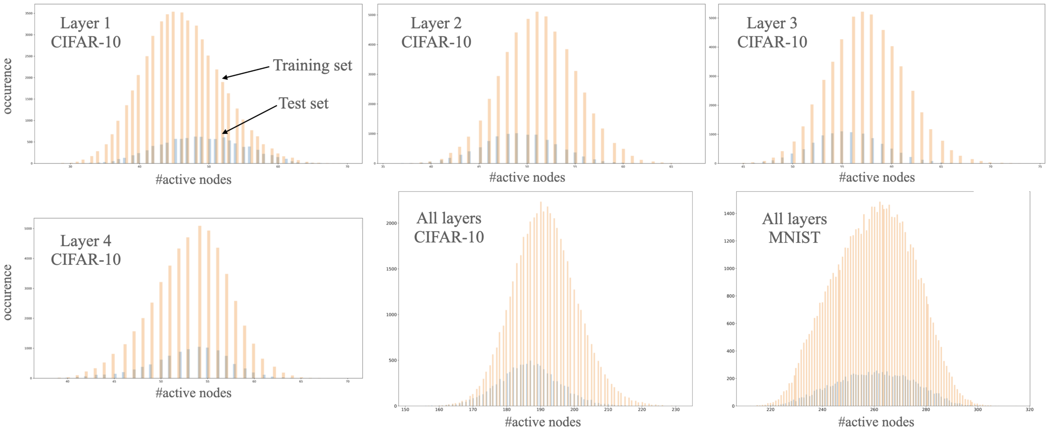
We now tighten the bound by discarding the assumption of independence from input and relating it to the structure of paths in the network. The above generic calculation assumes that every path materialised, a.k.a. every node has a positive activation along the path. Recent results [32] suggest that we can consider a more realistic case where the number of active nodes is significantly less than the number of nodes in the network (see Figure 1) thus our second bound takes into consideration the distribution of active nodes with the assumption of Gaussian. Let $T\left(x\right)={\sum }_i{n}_i\left(x\right)\in \mathcal{N}(\mu ,{\sigma }_T)$ be the number of active nodes for an input x with $n_i\left(x\right)$ as the number of active nodes in the i-th layer.

Theorem 2.

For $x\sim D$ and a biasless feed-forward ReLU network with a single output, with $w_{max}={max}_{w\in \theta }\left|w\right|$, with the number of active nodes $T\left(x\right)$ following a normal distribution $\mathcal{N}(\mu ,{\sigma }_T)$, the Forbenius norm of tangent sensitivity is upper bound by:

$$\mathsf{\Gamma }(N_{\theta },d_{in},k,\mu ,{\sigma }_T,w)=N_{\theta }{d}_{in}{\sigma }_T^{2(k-1)}\frac{2^{k-1}}{k^{2k}}\frac{{\left(\mathsf{\Gamma }(k/2)\right)}^2}{\Pi }{\widehat{\mathsf{\Psi }}}^2(k,\mu ,{\sigma }_T)w_{max}^{2(k-1)},$$

(2)

where $\widehat{\mathsf{\Psi }}(k,\mu ,{\sigma }_T)=\mathsf{\Psi }(-\frac{k-1}{2},\frac{1}{2},-\frac{{\mu }^2}{2{\sigma }_T^2})$ and Ψ is Krummer’s confluent hypergeometric function.

Theorem 2 is proved in Appendix B. The bound suggests an interesting connection between the depth of the network and the distribution of the number of active nodes. The depth of the network may overcome instability with appropriate weights and the mean number of active nodes. In order to probe this connection, we investigate the effect of depth, width, the norm of the weights and the number of active nodes in Section 4. Note, we have taken the maximal path count given the number of active units, however we do not take into account the distribution of activation patterns with the equivalent number of active hidden units. Thereby let us look into the expected sensitivity from a different angle to estimate tangent sensitivity as we focus on linear regions.

3.3. Distribution of Linear Regions

According to [42], the possible number of linear regions with the same activation pattern is $\left(\prod _{i=1}^{k-1}⎣{\frac{n_i}{d_{in}}⎦}^{d_{in}}\right)$ if we consider networks with a single output. In practice, the occurrence of every region is extremely rare. The following lemma suggests we investigate how the regions cover the input space and how the volume of convex activation regions is induced by the network.

Lemma 1.

For each element in an activation region $R(A;\theta )$, tangent sample sensitivity is identical.

Proof. 

By definition for any element in $R(A;\theta )$, the active neurons per layer are equal and therefore the positive paths for any input–output pair are identical thus tangent sample sensitivity is the same. □

It is worth mentioning that the lemma does not hold for linear regions. To see why, let us consider two neighbouring activation regions which differ only in one active neuron. The number of positive paths for elements in the neighbouring region will be higher if the neuron was not active and lower if the neuron was active in the first region. We refer to tangent sensitivity for elements in an activation region with $Sen{s}_{tan}(A;\theta )$. Without loss of generality we may assume that the input space is compact, thus every activation region has finite volume $\mathit{vol}\left(R\right(A;\theta \left)\right)<\infty$; therefore, the mean sensitivity for the compact input space is $Sen{s}_{tan}\left(\theta \right)={\sum }_{A\in {\mathit{A}}^{+}}\mathit{vol}\left(R(A;\theta )\right)Sen{s}_{tan}(A;\theta )$, where ${\mathit{A}}^{+}$ is the finite set of activation patterns of non-empty activation regions. As linear regions are represented by a finite set of linear inequalities their volume is exactly the volume of the bounding polytope. In the case of activation regions these polytopes are convex. Unfortunately, computing the volume of an explicit polytope is $\#P$-hard thus infeasible. In [43], the authors suggested an $O^{*}\left(d_{in}^4\right)$ (without additional terms, $O^{*}\left(d_{in}^3\right)$ in a special case [44]) algorithm for estimating the volume of a single convex body by simulated annealing. In a recent result [45], complexity was further improved with quantum oracles to $O^{*}\left(d_{in}^3\right)$, but the computations remain too expensive for tasks where neural networks have an advantage (e.g., high dimensional input dimension). It is worth noting that the convex body structure of a ReLU network is a well-defined subset, a hyperplane arrangement, therefore we are interested in the volume of many convex polytopes.

There are several ways to relax volume computation at the cost of accuracy. For example, the authors of [37] estimated the radius of the inspheres of linear regions by finding a point inside the polytope with the largest distance from the closest facet with solving a convex optimisation problem. This estimation measures the narrowness of a region and only valid for activation regions. However, none of the previously mentioned algorithms take into account the data distribution even if there are large regions without any support. Straightaway empirical estimation of the expected sensitivity may be difficult as Hoeffding’s inequality [46] $P{r}_{x\sim D}\left\{\right|\frac{1}{T}{\sum }_i^T{∥Sen{s}_{tan}(x_i;\theta )∥}_F^2-{∥Sen{s}_{tan}\left(\theta \right)∥}_F^2|>ϵ\}\le exp(-\frac{1}{2}\frac{{ϵ}^{2}T}{{\left(Sen{s}_{max,F}\right)}^2})$ can be meaningless if the maximal Frobenius norm of tangent sample sensitivity, $Sen{s}_{max,F}={max}_x{∥Sen{s}_{tan}(x;\theta )∥}_F^2$ is high. Note that the maximal sensitivity for a particular network is finite. Based on Lemma 1, tangent sensitivity depends on how the activation patterns distribute over the compact input space as:

$${\mathbf{E}}_{x\sim D}\left[{∥Sen{s}_{tan}(x;\theta )∥}_F^2\right]={\mathbf{E}}_{A\sim p(A;x,\theta )}\left[{∥Sen{s}_{tan}\left(A\right)∥}_F^2\right],$$

(3)

where we denote that the probability of an input is in an activation region with $p(A;x,\theta )$. Therefore we may estimate the upper bound of the tangent sensitivity as:

$$\parallel Sen{s}_{tan}{\left(\theta \right)\parallel }_F^2\le \sum _{A\in {\mathit{A}}^{+}}{N}_{\theta }{d}_{in}{\widehat{N}}^{2(k-1)}{w}_A^{2(k-1)}P(A;D,\theta ),$$

(4)

where ${\mathit{A}}^{+}$ is the finite set of non-empty activation pattern regions with corresponding active paths $\mathrm{path}\left(A\right)$ and $w_A={max}_{w\in \mathrm{path}\left(A\right)}\left|w\right|$ and $P(A;D,\theta )$ is the probability of the activation pattern A. It is worth mentioning that, if our assumptions for Theorem 2 hold, the upper bound will be ${\sum }_{A\in {\mathit{A}}^{+}}\mathsf{\Gamma }(N_{\theta },d_{in},k,\mu ,\sigma ,w_A)P(A;D,\theta )$.

The question remains: how can we determine the probability of a region without exactly computing the volume? As the number of activation regions may be larger than the size of an available dataset, practical calculation of relative frequency could be misleading. To overcome this we suggest a relaxation. By shallow networks, the independence of hidden units may seem an acceptable strong assumption, but in deep networks this is no longer the case. Let us assume the Markov property inside the network $p(A_{i,j};x,\theta )=p\left(A_{i,j}\right|\{h_{i-1,1}(x;\theta ),\dots ,h_{i-1,N_{i-1}}(x;\theta )\},\theta )\approx p\left(A_{i,j}\right|h_{i,j}(x;\theta ))$. As expected, the activation of a neuron depends on the preactivation of the neuron. Now, let us assume that for the l-th hidden unit (the j-th unit in the i-th layer) $log\frac{p(A_l=1|x;\theta )}{1-p(A_l=1|x;\theta )}\approx h_l(x;\theta )$ then for an input x and an activation pattern A the approximated probability is:

$$p(A=\{a_l;l\in \{1,2,\dots ,N\}\}|x;\theta )\approx {\Pi }_{l|a_l=1}\sigma \left(h_l(x;\theta )\right){\Pi }_{l|a_l=-1}(1-\sigma \left(h_l(x;\theta )\right),$$

(5)

where $\sigma \left(z\right)=1/(1+exp(-z\left)\right)$ denotes the sigmoid function. Note that this approximation is closely related to the margin distribution [25]. To relate the membership probability to the margin of individual neurons let us investigate a single neuron. The margin for a single neuron is defined as the minimal absolute preactivation for a finite set of inputs: ${\rho }_l\left(X\right):={min}_{x\in X}\left|h_l(x;\theta )\right|$. Because of the monotonicity of the sigmoid function we can explain the margin in a probabilistic sense with ${\widehat{\rho }}_l\left(X\right):={min}_{x\in X}|\sigma \left(h_l(x;\theta )\right)-0.5|$. The connection between $\rho$ and $\widehat{\rho }$ depends on the preactivation. For a neuron and input with positive preactivation, $\sigma \left(h_l(x;\theta )\right)$ is larger than $0.5$; similarly, for neurons with negative preactivation, $\sigma \left(h_l(x;\theta )\right)$ is smaller than $0.5$ therefore for points inside a region every element in (5) is larger than $0.5$. It is worth mentioning that it is possible that a point outside a region has higher membership probability than a point inside the region. In a further study we plan to examine more complex estimations of the membership probability.

3.4. Tangent Space Sensitivity and Generalisation

The authors of [1] established that fully trained (trained until zero error on the training set) neural networks show significantly more robust behaviour in the vicinity of the training data manifold, especially with random labels, in comparison to other subsets of the input space. They measure robustness on the training set by sampling around the training points and computing the Jacobian of the function realised by the network with regard to the input. In comparison, we would like to use our previously derived measures without exactly calculating the derivatives and estimate the empirical sensitivity on the training and on the test set. According to Lemma 1, inside an activation region tangent sample sensitivity is constant thus the volume of regions determines global stability.

The authors of [14] suggested measuring generalisation with the classification margin normalised by the spectral norm of the layer parameters. The Fisher–Rao norm was suggested in [23] where the state of a network was quantified with properties of the smooth loss manifold parametrised by the output of the network. Both methods rely on the true labels in comparison to our measures or the input–output sensitivity.

Based on our bounds we may introduce some practical estimations of the loss on the test set ($X_{te}$) based on various sensitivity measures and the loss on the training set ($X_{tr}$ with the corresponding target $Y_{tr}$):

• Layer-wise norm sensitivity, $Sen{s}_{tan}^1$ (Equation (1)): the bound does not depend on input, however the layer-wise $l_{\infty }$ norm of the parameters changes throughout learning therefore we may estimate the loss at time t (learning step t) based on the inverse change in maximal sensitivity (Equation (1)) and loss measured on the training set at time t:

  $${\widehat{l}}^1(X_{te};{\theta }^{\left(t\right)}):=\frac{Sen{s}_{tan}^1\left({\theta }^{(t-1)}\right))}{Sen{s}_{tan}^1\left({\theta }^{\left(t\right)}\right)}l\left(X_{tr},Y_{tr};{\theta }^{\left(t\right)}\right)=\frac{{\left({\Pi }_{i=1}^k{w}_{ma{x}_i}^{(t-1)}\right)}^2}{{\left({\Pi }_{i=1}^k{w}_{ma{x}_i}^{\left(t\right)}\right)}^2}l\left(X_{tr},Y_{tr};{\theta }^{\left(t\right)}\right),$$

  (6)

  where $w_{ma{x}_i}^{\left(t\right)}$ is $l_{\infty }$ norm in the i-th layer at time t. The missing parts of (Equation (1)) are invariable throughout learning.
• Maximal sensitivity, $Sen{s}_{tan}^2$ (Equation (2)): similarly, we may estimate test loss based on the distribution of the number of active nodes:

  $${\widehat{l}}^2(X_{te};\theta ):=\frac{{\psi }^{*}(k,{\mu }_{te},{\sigma }_{te})}{{\psi }^{*}(k,{\mu }_{tr},{\sigma }_{tr})}l(X_{tr},Y_{tr};\theta ),$$

  (7)

  where ${\psi }^{*}(k,\mu ,\sigma )={\sigma }^{2(k-1)}\mathsf{\Psi }{(-(k-1)/2,1/2,-{\mu }^2/\left(2{\sigma }^2\right))}^2$ and the corresponding normal distributions are $\mathcal{N}({\mu }_{tr},{\sigma }_{tr})$ and $\mathcal{N}({\mu }_{te},{\sigma }_{te})$ for the training and the test sets, respectively. Note that the missing parts of (Equation (2)) are invariable if the graph of the network is fixed. At any state of the network, the difference between the estimated sensitivity is based only on how the distribution of the number of active neurons differs in the two sets and the depth of the network while concealing the difference in activation patterns given the sets.
• Empirical sensitivity, $Sen{s}_{tan}^3$ (Equation (3)): assuming the empirical estimation of $p(A;\theta )$ in (Equations (2) and (5)) we define empirical tangent sensitivity as:

  $$\widehat{S}(X;\theta )=\sum _{A_i\in {\mathit{A}}^{+}}{p}_{x\in X}(A_i;\theta )Sen{s}_{tan}(A_i;\theta ).$$
  The corresponding estimation of test loss:

  $${\widehat{l}}^3(X_{te};\theta ):=\frac{\widehat{S}(X_{te};\theta )}{\widehat{S}(X_{tr};\theta )}l(X_{tr},Y_{tr};\theta ).$$

  (8)

In addition to the distribution of activation regions, the above estimations coincide with previous results that connect generalisation to the norm of network parameters [14], to maximal capacity [6,19,36] and to margin distribution [25].

4. Experiments

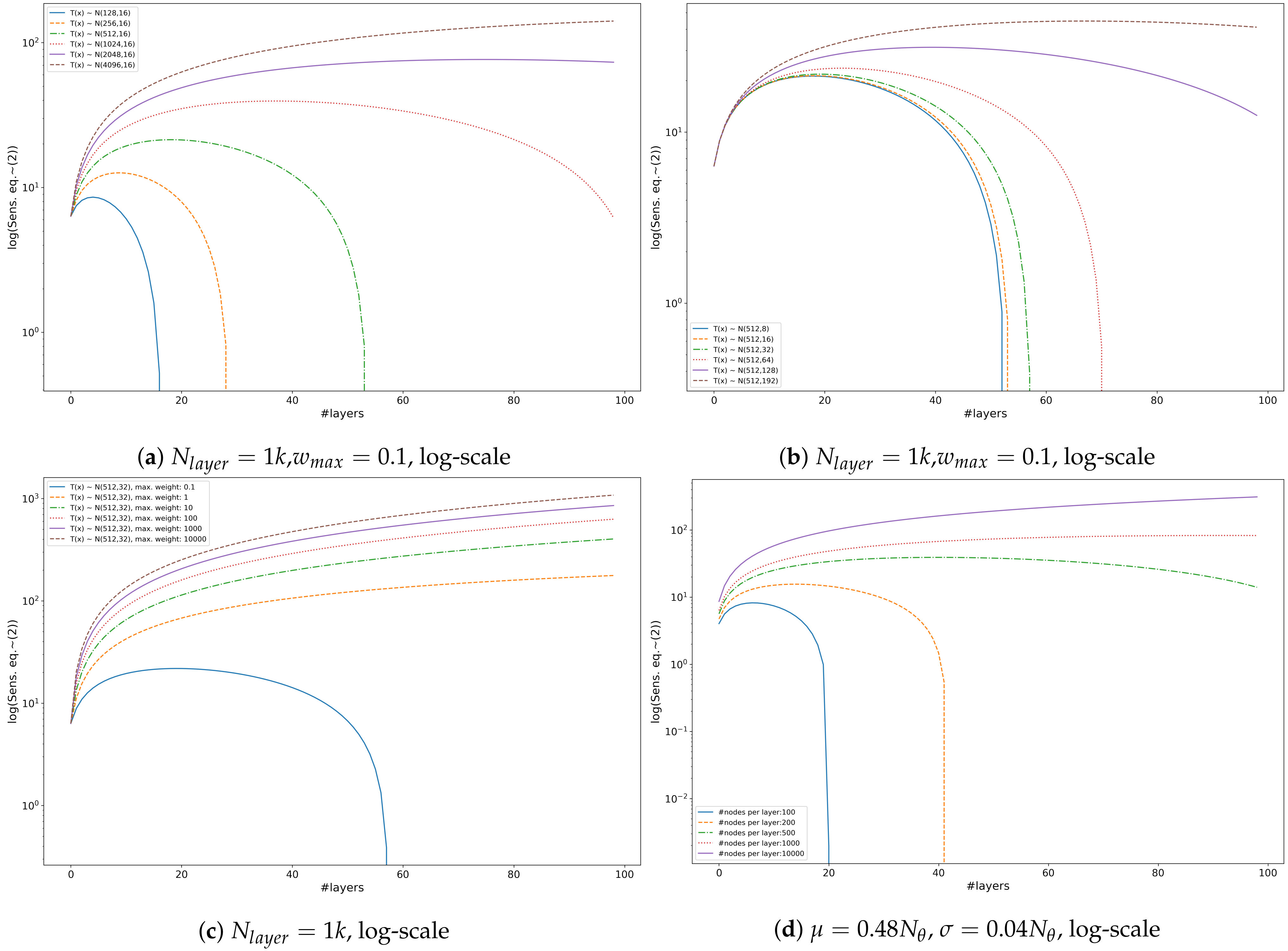
Building upon the discussion in Section 3.2 and Section 3.4, we experiment with feed-forward fully-connected ReLU networks. Based on the analysis of (Equations (1) and (2)) we observed that the most important factor in sensitivity is the depth of the network followed by the layer-wise norm of the parameters and the empirical variance of number of active neurons in the network, for details see Figure 2. Tangent sensitivity per sample depends on the number of active paths between the input and the output, and if we increase the number of nodes per layer we increase the possible number of active paths. The number of nodes per layer only affects the bounds via the number of parameters ($N_{\theta }$). Additionally, we found that the upper bound of the tangent sensitivity with proper regularisation (e.g., low norm) after reaching a certain depth starts to decrease, supporting one of the fundamental phenomena of deep learning; deeper networks may generalise better.

Furthermore, we investigated how empirical accuracy and cross-entropy loss related to tangent sensitivity in the case of feed-forward fully-connected ReLU networks with four hidden layers on the CIFAR-10 [38] dataset. The dataset consists 60k tiny images in ten different classes (airplanes, cars, birds, cats, deer, dogs, frogs, horses, ships, and trucks). The dataset has five 10k sized training batches and one 10k sized testing batch. Additional experiments with detailed description about the experiments and the implementation can be found in Appendix C. We implemented the measures in Section 3.4 and three additional measures:

• Input-output sensitivity [1]: In case of binary classification and for an input set X, input sensitivity is defined as

  $$S_{Jac}(X;\theta )=E_{x\in X}[\parallel \frac{\partial f(x;\theta )}{\partial x}{\parallel }_2]$$

  therefore we may estimate the loss at time t (learning step t) based on the sensitivity on the training and the test set and the loss measured on the training set at time t:

  $$l^4(X_{te};\theta ):=\frac{S_{Jac}(X_{te};\theta )}{S_{Jac}(X_{tr};\theta )}l(X_{tr},Y_{tr};\theta ).$$

  (9)
• Fisher-Rao norm [23]: The authors proposed a measure (Theorem 3.1) in case of smooth loss with known labeling as

  $$S_{FR}(X,Y;\theta )={(k+1)}^2{E}_{x,y}[<\frac{\partial l\left(f\right(x;\theta ),y)}{\partial f(x;\theta )},f(x;\theta ){>}^2].$$
  The measure depends on the input labels therefore we need a slight modification with replacing the loss with the sum of loss over all ten classes:

  $$S_{FR}(X;\theta )=\sum _{j=1}^{10}{E}_x[<\frac{\partial l\left(f\right(x;\theta ),j)}{\partial f(x;\theta )},f(x;\theta ){>}^2].$$
  We are only interested in the change of the measure therefore we also remove the constant part. We may estimate the loss on the test set by

  $$l^5(X_{te};\theta ):=\frac{S_{FR}(X_{te};\theta )}{S_{FR}(X_{tr};\theta )}l(X_{tr},Y_{tr};\theta ).$$

  (10)
• Spectral norm [14]: the authors suggest spectrally normalised margin complexity to measure generalisation in case of multiclass classification as

  $$S_{Spect}(X,Y;\theta )=\frac{f{(x;\theta )}_y-{max}_{i\ne y}f{(x;\theta )}_j}{S_{Spect}\left(\theta \right){\parallel X\parallel }_2/n}$$

  where $f{(x;\theta )}_y-maxi\ne yf{(x;\theta )}_j$ represents the margin of a sample with $f{(x;\theta )}_y$ as the y-th output of the network and with zero matrices as reference matrices (Equation (1.2) in [14])

  $$S_{Spect}\left(\theta \right)={\Pi }_{i=1}^k{\parallel W_i\parallel }_{\sigma }.$$
  As the measure depends on the input label we modified the measure by removing the margin motivated by the fact that on the training set the margin can be misleading as the models may reach high accuracy fast. Additionally, we are only interested in the change of the measure therefore we also remove the norm of the input as it is constant throughout our experiments. The final estimation is similarly to the layer-wise $l_{\infty }$ norm:

  $$l^6(X_{te};{\theta }^{\left(t\right)}):=\frac{S_{Spect}\left({\theta }^{(t-1)}\right))}{S_{Spect}\left({\theta }^{\left(t\right)}\right)}l\left(X_{tr},Y_{tr};{\theta }^{\left(t\right)}\right).$$

  (11)

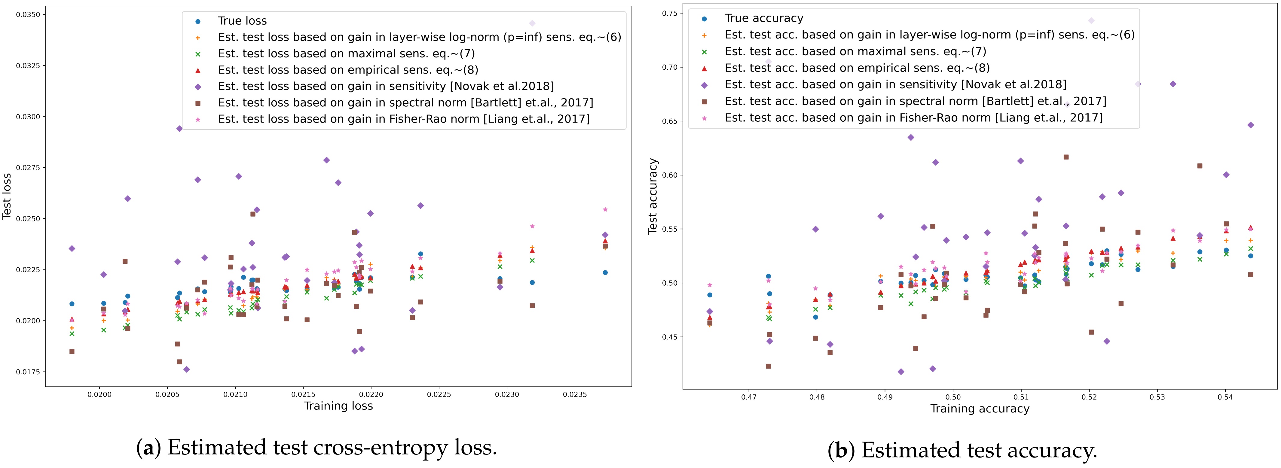
During the experiments we used the five training batches of CIFAR-10 as a training set and the test batch as a test set. The network parameters were optimised with stochastic gradient descent with weight decay. The results in Figure 3 show that our previously introduced measures may estimate changes in the empirical generalisation gap to some extent. We found that the upper bound of tangent sensitivity may indicate an exponentially large change in loss because of the layer-wise $l_{\infty }$ norm of the parameters thus we modified our estimation by taking the logarithm of sensitivity instead of simply taking (Equation (1)) in (Equation (6)). All estimations performed very similarly. The lowest Mean Absolute Error (MAE) for cross-entropy loss and accuracy were achieved by empirical sensitivity (Equation (8)) and layer-wise log-norm sensitivity (Equation (6)) respectively.

We measured the quality of the estimated test cross-entropy loss and test accuracy with Mean Absolute Error (MAE), for details see

Table 1. Mean Absolute Error (MAE) of estimated test cross-entropy loss and test accuracy of ReLU networks on different states on the CIFAR-10 dataset based on layer-wise log-norm ($l_{\infty })$ (Equation (6)), maximal (Equation (7)), empirical tangent sensitivity (Equation (8)), change in input–output sensitivity (Equation (9)), in Fisher-Rao norm (Equation (10)) and in spectral norm (Equation (11)).

Estimation	Cross-Entropy	Accuracy
Layer-wise log-norm (p = inf) sens. (Equation (6))	$5.3\times {10}^{-4}$	$9.2\times {10}^{-3}$
Maximal sens. (Equation (7))	$7.7\times {10}^{-4}$	$9.8\times {10}^{-3}$
Empirical sens. (Equation (8))	$4.2\times {10}^{-4}$	$1.1\times {10}^{-2}$
Change in sens. (Equation (9))	$2.7\times {10}^{-3}$	$7.3\times {10}^{-2}$
Change in spectral norm (Equation (11))	$1.2\times {10}^{-3}$	$3.3\times {10}^{-2}$
Change in Fisher-Rao norm (Equation (10))	$6.3\times {10}^{-4}$	$1.5\times {10}^{-2}$

. The lowest MAE cross-entropy loss and accuracy were achieved by empirical sensitivity (Equation (8)) and layer-wise log-norm sensitivity (Equation (6)) respectively. The Fisher–Rao norm outperformed both the spectral norm and the input–output sensitivity in both estimations and achieved a lower difference in estimating the cross-entropy than the maximal sensitivity.

5. Conclusions

In this paper we proposed measures of sensitivity to perturbations, to capture the connection between the input and the output regarding the gradient mapping, in feed-forward neural networks without considering any label. To calculate the sensitivity of the network, we estimated the change to small perturbations in the tangent vectors by taking the derivative of the tangent vectors with regard to the input. Our main hypothesis was that if the network was optimised with first order methods, the stability of optimisation is related to the gradient mapping. We found that tangent sensitivity in ReLU networks is related to the number of active paths between input–output pairs and the norm of the weight parameters. We also found that tangent sensitivity is constant inside activation regions and the expected sensitivity is related to the distribution of the activation regions. As was shown in the works [47,48,49,50], generalisation error is connected to the mutual information between the input and the output; therefore, our plan is to examine this connection to mutual information in a future work, e.g., the convergence of the distribution of activation regions during learning, and to generalise the results to activation functions with bounded first derivatives. In addition, our initial assumptions merit further investigation of residual, convolutional and recurrent network structures together with autoencoders. Furthermore, our work was limited to smooth transformations in input omitting important non smooth augmentation methods, e.g., image mirroring. A natural next step would be to connect tangent sensitivity with information geometry as feedforward neural networks usually have a Riemannian metric structure [8,23] and to examine generalisation induced by the differential structure while constructing regularisation methods to minimise tangent sensitivity, suggesting non-trivial network structures and exploiting invariance properties of Fisher information [11], among others.

References

- Novak, R.; Bahri, Y.; Abolafia, D.A.; Pennington, J.; Sohl-Dickstein, J. Sensitivity and generalisation in neural networks: An empirical study. In Proceedings of the ICLR’18, Vancouver, BC, Canada, 20 April–3 May 2018. [Google Scholar]
- Sontag, E.D. VC dimension of neural networks. NATO ASI Ser. F Comput. Syst. Sci. 1998, 168, 69–96. [Google Scholar]
- Bartlett, P.L.; Maass, W. Vapnik-Chervonenkis dimension of neural nets. In The Handbook of Brain Theory and Neural Networks; MIT Press: Cambridge, MA, USA, 2003; pp. 1188–1192. [Google Scholar]
- Liu, T.; Lugosi, G.; Neu, G.; Tao, D. Algorithmic stability and hypothesis complexity. In Proceedings of the 34th International Conference on Machine Learning, Sydney, Australia, 6–11 August 2017; Volume 70, pp. 2159–2167. [Google Scholar]
- Rolnick, D.; Tegmark, M. The power of deeper networks for expressing natural functions. arXiv 2017, arXiv:1705.05502. [Google Scholar]
- Lin, H.W.; Tegmark, M. Why does deep and cheap learning work so well? arXiv 2016, arXiv:1608.08225. [Google Scholar] [CrossRef] [Green Version]
- Stoudenmire, E.; Schwab, D.J. Supervised learning with tensor networks. In Advances in Neural Information Processing Systems, Proceedings of the NIPS 2016, Barcelona, Spain, 5–10 December 2016; Curran Associates Inc.: North Adams, MA, USA, 2016; pp. 4799–4807. [Google Scholar]
- Amari, S.I. Neural learning in structured parameter spaces-natural Riemannian gradient. In Advances in Neural Information Processing Systems, Proceedings of the NIPS 1996, Denver, CO, USA, 3–5 December 1996; MIT Press: Cambridge, MA, USA, 1996; pp. 127–133. [Google Scholar]
- Kanwal, M.; Grochow, J.; Ay, N. Comparing information-theoretic measures of complexity in Boltzmann machines. Entropy 2017, 19, 310. [Google Scholar] [CrossRef]
- Jacot, A.; Gabriel, F.; Hongler, C. Neural tangent kernel: Convergence and generalisation in neural networks. In Advances in Neural Information Processing Systems, Proceedings of the NIPS 2018, Montreal, QC, USA, 3–8 December 2018; MIT Press: Cambridge, MA, USA, 2018; pp. 8571–8580. [Google Scholar]
- Ay, N.; Jost, J.; Vân Lê, H.; Schwachhöfer, L. Information Geometry; Springer: Berlin/Heidelberg, Germany, 2017; Volume 64. [Google Scholar]
- Neyshabur, B.; Li, Z.; Bhojanapalli, S.; LeCun, Y.; Srebro, N. Towards understanding the role of over-parametrisation in generalisation of neural networks. In Proceedings of the ICLR 2018, Vancouver, BC, USA, 30 April–3 May 2018. [Google Scholar]
- Du, S.S.; Zhai, X.; Poczos, B.; Singh, A. Gradient descent provably optimises over-parameterised neural networks. arXiv 2018, arXiv:1810.02054. [Google Scholar]
- Bartlett, P.L.; Foster, D.J.; Telgarsky, M.J. Spectrally-normalised margin bounds for neural networks. In Advances in Neural Information Processing Systems 30, Proceedings of the NIPS 2017, Long Beach, CA, USA, 4–9 December 2017; Curran Associates Inc.: North Adams, MA, USA, 2017; pp. 6240–6249. [Google Scholar]
- Krogh, A.; Hertz, J.A. A simple weight decay can improve generalisation. In Advances in Neural Information Processing Systems, Proceedings of the NIPS 1992, Denver, CO, USA, 2–5 December 1992; Morgan Kaufmann Publishers Inc.: San Francisco, CA, USA, 1992; pp. 950–957. [Google Scholar]
- Neyshabur, B.; Tomioka, R.; Srebro, N. In search of the real inductive bias: On the role of implicit regularisation in deep learning. In Proceedings of the ICLR’14, Banff, AB, Canada, 14–16 April 2014. [Google Scholar]
- Zhang, C.; Bengio, S.; Hardt, M.; Recht, B.; Vinyals, O. Understanding deep learning requires rethinking generalisation. arXiv 2016, arXiv:1611.03530. [Google Scholar]
- Srivastava, N.; Hinton, G.; Krizhevsky, A.; Sutskever, I.; Salakhutdinov, R. Dropout: A simple way to prevent neural networks from overfitting. J. Mach. Learn. Res. 2014, 15, 1929–1958. [Google Scholar]
- Cao, Y.; Gu, Q. Generalisation bounds of stochastic gradient descent for wide and deep neural networks. In Advances in Neural Information Processing Systems 32, Proceedings of the NIPS 2019, Vancouver, BC, Canada, 8–14 December 2019; Curran Associates Inc.: North Adams, MA, USA, 2019; pp. 10835–10845. [Google Scholar]
- Perez, L.; Wang, J. The effectiveness of data augmentation in image classification using deep learning. arXiv 2017, arXiv:1712.04621. [Google Scholar]
- Wilson, A.C.; Roelofs, R.; Stern, M.; Srebro, N.; Recht, B. The marginal value of adaptive gradient methods in machine learning. In Advances in Neural Information Processing Systems 30, Proceedings of the NIPS 2017, Long Beach, CA, USA, 4–9 December 2017; Curran Associates Inc.: North Adams, MA, USA, 2017; pp. 4148–4158. [Google Scholar]
- Keskar, N.S.; Socher, R. Improving generalisation performance by switching from adam to sgd. arXiv 2017, arXiv:1712.07628. [Google Scholar]
- Liang, T.; Poggio, T.; Rakhlin, A.; Stokes, J. Fisher-rao metric, geometry, and complexity of neural networks. arXiv 2017, arXiv:1711.01530. [Google Scholar]
- Dinh, L.; Pascanu, R.; Bengio, S.; Bengio, Y. Sharp minima can generalise for deep nets. In Proceedings of the 34th International Conference on Machine Learning, Sydney, Australia, 6–11 August 2017; Volume 70, pp. 1019–1028. [Google Scholar]
- Jiang, Y.; Krishnan, D.; Mobahi, H.; Bengio, S. Predicting the generalisation gap in deep networks with margin distributions. In Proceedings of the ICLR’19, New Orleasns, LA, USA, 6–9 May 2019. [Google Scholar]
- Goodfellow, I.J.; Shlens, J.; Szegedy, C. Explaining and harnessing adversarial examples. arXiv 2014, arXiv:1412.6572. [Google Scholar]
- Nagarajan, V.; Kolter, J.Z. Uniform convergence may be unable to explain generalisation in deep learning. In Advances in Neural Information Processing Systems 32, Proceedings of the NIPS 2019, Vancouver, BC, Canada, 8–14 December 2019; Wallach, H., Larochelle, H., Beygelzimer, A., d’Alché-Buc, F., Fox, E., Garnett, R., Eds.; Curran Associates, Inc.: North Adams, MA, USA, 2019; pp. 11615–11626. [Google Scholar]
- Werpachowski, R.; György, A.; Szepesvári, C. Detecting overfitting via adversarial examples. In Advances in Neural Information Processing Systems 32, Proceedings of the NIPS 2019, Vancouver, BC, Canada, 8–14 December 2019; Curran Associates, Inc.: North Adams, MA, USA, 2019; pp. 7856–7866. [Google Scholar]
- Zhang, C.; Bengio, S.; Hardt, M.; Recht, B.; Vinyals, O. Understanding deep learning (still) requires rethinking generalisation. Commun. ACM 2021, 64, 107–115. [Google Scholar] [CrossRef]
- Beritelli, F.; Capizzi, G.; Sciuto, G.L.; Napoli, C.; Scaglione, F. Rainfall estimation based on the intensity of the received signal in a LTE/4G mobile terminal by using a probabilistic neural network. IEEE Access 2018, 6, 30865–30873. [Google Scholar] [CrossRef]
- Sciuto, G.L.; Napoli, C.; Capizzi, G.; Shikler, R. Organic solar cells defects detection by means of an elliptical basis neural network and a new feature extraction technique. Optik 2019, 194, 163038. [Google Scholar] [CrossRef]
- Hanin, B.; Rolnick, D. Deep relu networks have surprisingly few activation patterns. In Advances in Neural Information Processing Systems 32, Proceedings of the NIPS 2019, Vancouver, BC, Canada, 8–14 December 2019; Curran Associates, Inc.: North Adams, MA, USA, 2019; pp. 359–368. [Google Scholar]
- Raghu, M.; Poole, B.; Kleinberg, J.; Ganguli, S.; Dickstein, J.S. On the expressive power of deep neural networks. In Proceedings of the 34th International Conference on Machine Learning, Sydney, Australia, 6–11 August 2017; Volume 70, pp. 2847–2854. [Google Scholar]
- Arora, S.; Ge, R.; Neyshabur, B.; Zhang, Y. Stronger generalisation bounds for deep nets via a compression approach. arXiv 2018, arXiv:1802.05296. [Google Scholar]
- Neyshabur, B.; Salakhutdinov, R.R.; Srebro, N. Path-SGD: Path-Normalised Optimisation in Deep Neural Networks. In Advances in Neural Information Processing Systems, Proceedings of the NIPS 2015, Montreal, QC, Canada, 7–12 December 2015; Curran Associates, Inc.: North Adams, MA, USA, 2015. [Google Scholar]
- Neyshabur, B.; Bhojanapalli, S.; McAllester, D.; Srebro, N. Exploring generalisation in deep learning. In Advances in Neural Information Processing Systems 30, Proceedings of the NIPS 2017, Long Beach, CA, USA, 4–9 December 2017; Curran Associates Inc.: North Adams, MA, USA, 2017; pp. 5947–5956. [Google Scholar]
- Zhang, X.; Wu, D. Empirical Studies on the Properties of Linear Regions in Deep Neural Networks. arXiv 2020, arXiv:2001.01072. [Google Scholar]
- Krizhevsky, A.; Hinton, G. Learning Multiple Layers of Features from Tiny Images; Technical Report; MIT Press: Cambridge, MA, USA; NYU: New York, NY, USA, 2009. [Google Scholar]
- Devroye, L.; Györfi, L.; Lugosi, G. A Probabilistic Theory of Pattern Recognition; Springer Science & Business Media: Berlin/Heidelberg, Germany, 2013; Volume 31. [Google Scholar]
- Carlini, N.; Wagner, D. Adversarial examples are not easily detected: Bypassing ten detection methods. In Proceedings of the 10th ACM Workshop on Artificial Intelligence and Security, Dallas, TX, USA, 3 November 2017; pp. 3–14. [Google Scholar]
- LeCun, Y.; Bottou, L.; Bengio, Y.; Haffner, P. Gradient-based learning applied to document recognition. Proc. IEEE 1998, 86, 2278–2324. [Google Scholar] [CrossRef] [Green Version]
- Montufar, G.F.; Pascanu, R.; Cho, K.; Bengio, Y. On the number of linear regions of deep neural networks. In Advances in Neural Information Processing Systems, Proceedings of the NIPS 2014, Montreal, QA, Canada, 8–13 December 2014; Curran Associates Inc.: North Adams, MA, USA, 2014. [Google Scholar]
- Lovász, L.; Vempala, S. Simulated annealing in convex bodies and an O*(n4) volume algorithm. J. Comput. Syst. Sci. 2006, 72, 392–417. [Google Scholar] [CrossRef] [Green Version]
- Cousins, B.; Vempala, S. A practical volume algorithm. Math. Program. Comput. 2016, 8, 133–160. [Google Scholar] [CrossRef]
- Chakrabarti, S.; Childs, A.M.; Hung, S.H.; Li, T.; Wang, C.; Wu, X. Quantum algorithm for estimating volumes of convex bodies. arXiv 2019, arXiv:1908.03903. [Google Scholar]
- Hoeffding, W. Probability inequalities for sums of bounded random variables. In The Collected Works of Wassily Hoeffding; Springer: Berlin/Heidelberg, Germany, 1994; pp. 409–426. [Google Scholar]
- Russo, D.; Zou, J. Controlling bias in adaptive data analysis using information theory. In Artificial Intelligence and Statistics, Proceedings of the 19th International Conference on Artificial Intelligence and Statistics, Cadiz, Spain, 9–11 May 2016; PMLR: Westminster, UK, 2016; pp. 1232–1240. [Google Scholar]
- Russo, D.; Zou, J. How much does your data exploration overfit? Controlling bias via information usage. IEEE Trans. Inf. Theory 2019, 66, 302–323. [Google Scholar] [CrossRef] [Green Version]
- Xu, A.; Raginsky, M. Information-theoretic analysis of generalisation capability of learning algorithms. In Advances in Neural Information Processing Systems 30, Proceedings of the NIPS 2017, Long Beach, CA, USA, 4–9 December 2017; Curran Associates Inc.: North Adams, MA, USA, 2017. [Google Scholar]
- Neu, G.; Lugosi, G. Generalisation Bounds via Convex Analysis. arXiv 2022, arXiv:2202.04985. [Google Scholar]
- Winkelbauer, A. Moments and absolute moments of the normal distribution. arXiv 2012, arXiv:1209.4340. [Google Scholar]
- Ioffe, S.; Szegedy, C. Batch normalisation: Accelerating deep network training by reducing internal covariate shift. arXiv 2015, arXiv:1502.03167. [Google Scholar]
- Kingma, D.; Ba, J. Adam: A method for stochastic optimisation. arXiv 2014, arXiv:1412.6980. [Google Scholar]
Figure 1.
Histogram of active neurons per input (the number of active nodes in the network) after 50 epochs on the training and on the test set in a 4-layer feed-forward ReLU network with 100 neurons per layer on CIFAR-10 [38] and on MNIST [41].
Figure 2.
Change in upper bound (Equation (2)) induced by mean (a), variance (b), maximal norm (c) and width of layers (d).
Figure 3.
Estimated test cross-entropy loss (a) and test accuracy (b) on the CIFAR-10 dataset with the ReLU network on different states (trained with stochastic gradient descent with batch size of 64, learning rate with and weight decay with ) based on layer-wise log-norm ( (Equation (6)), maximal (Equation (7)), empirical tangent sensitivity (Equation (8)), input–output sensitivity (Equation (9)), Fisher–Rao norm (Equation (10)) and spectral norm (Equation (11)).