Article

The IRC Indices of Transformation and Derived Graphs

1
School of Intelligent Manufacturing, Zhanjiang University of Science and Technology, Zhanjiang 524300, China
2
School of Mathematics and Information Sciences, Guangzhou University, Guangzhou 510006, China
3
Department of Social Sciences, Maoming Polytechnic, Maoming 525000, China
4
Donát Bánki Faculty of Mechanical and Safety Engineering, Obuda University, Népszínház str. 8, H-1081 Budapest, Hungary
*
Author to whom correspondence should be addressed.
These authors contributed equally to this work.
Mathematics 2022, 10(7), 1111; https://doi.org/10.3390/math10071111
Submission received: 22 February 2022 / Revised: 23 March 2022 / Accepted: 28 March 2022 / Published: 30 March 2022
(This article belongs to the Special Issue Graph Theory and Applications)

Abstract

:
An irregularity index I R ( Γ ) of a graph Γ is a nonnegative numeric quantity (i.e., I R ( Γ ) 0 ) such that I R ( Γ ) = 0 iff Γ is a regular graph. In this paper, we show that I R C closely correlates with the normal boiling point T b p and the standard heat of formation Δ H f o of lower benzenoid hydrocarbons. The correlation models that fit the data efficiently for both T b p and Δ H f o are linear. We develop further mathematical properties of I R C by calculating its exact expressions for the recently introduced transformation graphs as well as certain derived graphs, such as the total graph, semi-total point graph, subdivision graph, semi-total line graph, double, strong double, and extended double cover graphs. Some open problems are proposed for further research on the I R C index of graphs.

1. Introduction

In modern chemistry, the dependence of the physicochemical properties of a compound on its chemical structure is a cornerstone idea. Studying this dependence up to its full potential is rather challenging [1]. Unavailability of experimental data is one of the common challenges encountered in unveiling this dependence. A lot of research [2,3,4,5,6] has been conducted so far to estimate the missing data. Modern tools such as machine learning [7] and graph signal processing (GSP) [8] have recently been employed to address this data retrieval. Molecular descriptors [9,10,11] are one of the contemporary tools to predict diverse psychochemical features of a chemical compound. Graph-theoretic descriptors are an important class of descriptors that transform a chemical compound into a graph; diverse graph-theoretic tools are then employed to retrieve the dependence. A lot of available research [12,13,14] shows that these graph-based invariants, which are easily computable, efficiently encrypt a significantly higher level of structural information of chemical compounds.
Diverse classes of topological indices include degree-based indices, which have significantly better efficiency. An irregularity index I R ( Γ ) of a graph Γ is a nonnegative numeric quantity (i.e., I R ( Γ ) 0 ), such that I R ( Γ ) = 0 iff Γ is a regular graph. Degree-based irregularity indices have diverse application in QSPR/QSAR modeling [15]. Thus, their mathematical properties have been studied extensively. For instance, Ascioglu and Cangul [16] studied the σ irregularity index and the forgotten index of subdivision and r-subdivision graphs. Réti [17] studied upper and lower bounds on various degree-based irregularity indices, such as the sigma index, irregularity indices based on Zagreb, forgotten topological indices, and so on. In the same work, Réti [17] introduced the I R C index. This paper presents its potential applicability in QSPR/QSAR modeling of compounds. We also studied the I R C index for various transformation and derived graphs.
This paper is organized as follows: Section 2 presents definitions and preliminary results required in later sections. Section 3 applies the I R C index in QSAR modeling of physicochemical properties of chemical compounds. Section 4 and Section 5 present results on the I R C index of transformation graphs and derived graphs, respectively. Section 6 concludes the paper and exhibits some open problems relating to the I R C index.

2. Preliminaries

A simple graph G is an ordered pair G = ( V , E ) , where V is the set of points called vertices and E V 2 is the set of lines called edges. The cardinality n = V (respectively, e = E ) of E is called the order (respective size) of G. Two vertices, u , v V ( G ) , respectively, (edges e , f E ( G ) ) are said to be adjacent if u v E ( G ) (respectively, e and f share a common end-vertex). In that case, we denote adjacency with y z or e f . A vertex u V ( G ) and an edge e E ( G ) are called incident and written as u e if u is one of the end-vertex of e. The number of vertices adjacent to a vertex u is known as the degree of u and written as d ( u ) . A graph is called bipartite if it contains no cycle of added length. We refer the reader to a book on molecular topology by Diudea et al. [18].
A topological invariant I R ( G ) of graph G is said to have an irregularity index if I R ( G ) 0 and I R ( G ) = 0 iff G is regular. Based on its defining structure, an irregularity index could either be eigenvalues-based or degree-based.
The first ever proposed irregularity index is eigenvalues-based and known as the Collatz–Sinogowitz irregularity index [19], which determines the irregularity of a graph. For a n-vertex e-edge graph G ( n , e ) , it is defined as follows:
C S ( G ) = λ ( G ) 2 e n ,
where λ is the spectral radius of the adjacency matrix of G. Because of the lower computational complexity, irregularity indices are mostly degree-based. In 1992, Bell [20] introduced a degree-based irregularity index known as the variance of degree V a r ( G ) , which has significant applications in chemistry. For a ( n , e ) graph G, it is defined as
V a r ( G ) = 1 n u V ( G ) ( d ( u ) ) 2 1 n 2 u V ( G ) d ( u ) 2 = 1 n u V ( G ) ( d ( u ) ) 2 2 e n 2 .
In 1997, Albertson introduced another degree-based irregularity index, known as Albertson’s irregularity index. It is defined as
A L ( G ) = u v E ( G ) d ( u ) d ( v ) .
By extending Albertson’s irregularity index, Gutman et al. [21] introduced the sigma index.
σ ( G ) = u v E ( G ) ( d ( u ) d ( v ) ) 2 .
A topological index T is a map from the set of simple connected graph ∑ to the real set (i.e., T : ), and it has significant applications in chemistry. One of the earliest degree-based topological indices are the Zagreb indices. Gutman and Trinajstić [22] introduced the two Zagreb indices back in 1972 while working on the total π -electronic energy of benzenoid hydrocarbons in theoretical chemistry. They have have been employed in various chemical application since then (see for instance, Gutman and Das [23] and Gutman [24]). For a graph G, the two Zagreb indices are defined as follows:
M 1 ( G ) = u v E ( G ) d ( u ) + d ( v ) = u V ( G ) d 2 ( u ) , M 2 ( G ) = u v E ( G ) d ( u ) d ( v ) .
Furtula and Gutman [25] proposed a degree-based structure descriptor, which they called the forgotten topological index. It is defined as:
F ( G ) = u V ( G ) d 3 ( u ) .
In connection with the Zagreb indices, several new irregularity indices have been established. Two of those Zagreb-related irregularity indices are the following [15,26]:
I R M 1 ( G ) = M 1 ( G ) n 2 e n = V a r ( G ) M 1 ( G ) n + 2 e n 1 .
I R M 2 ( G ) = M 2 ( G ) n 2 e n .
Moreover, based on a degree-based quantity proposed in [27], Réti [17] introduced the following irregularity index:
I R C ( G ) = u V ( G ) d 3 ( u ) 2 e n u V ( G ) d 2 ( u ) = F ( G ) 2 e n M 1 ( G ) 0 .
This paper focuses on this new irregularity index (i.e., I R C index) and presents its potential applicability in modeling physico-chemical properties of benzenoid hydrocarbons. Then, further mathematical properties of the I R C index are studied.
For an edge e = x y E ( G ) , the degree of e is defined as d ( e ) = d ( u ) + d ( v ) 2 . Based on degrees of edges, Ilić and Zhou [28] proposed the reformulated Zagreb indices. For a graph G, the reformulated first Zagreb index is defined as follows:
E M 1 ( G ) = f E ( G ) d 2 ( f ) .
The reformulated second Zagreb index is defined as follows:
E M 2 ( G ) = e , f E ( G ) , e f d ( e ) d ( f ) .
Similarly, an edge version of the forgotten index, also called the reformulated forgotten index, of G is defined as follows:
E F ( G ) = f E ( G ) d 3 ( f ) .
Recently, Ranjini et al. [29] introduced certain redefined versions of the Zagreb indices. The redefined first, second, and third Zagreb indices are defined as follows:
R e Z G 1 ( G ) = u v E ( G ) d ( u ) + d ( v ) d ( u ) d ( v ) , R e Z G 2 ( G ) = u v E ( G ) d ( u ) d ( v ) d ( u ) + d ( v ) , R e Z G 3 ( G ) = u v E ( G ) d ( u ) d ( v ) [ d ( u ) + d ( v ) ] .
Now we introduce some derived graphs based on different graph operations. The total graph T ( G ) of a graph G was introduced by Behzad [30] in 1967, and it has the vertex set V T ( G ) = V ( G ) E ( G ) , such that y z , y e , e f E T ( G ) iff y z , z e or e f are adjacent/incident in G.
Sampathkumar and Chikkodimath [31] extended the concept of the total graph and put forward two semi-total point and line graphs. The semi-total point graph T 1 ( G ) has the vertex set V T 1 ( G ) = V ( G ) E ( G ) , and any two vertices y , z V T 1 ( G ) are adjacent iff:
(i)
u , v V ( G ) such that u v in G, or;
(ii)
u V ( G ) , e E ( G ) or vice versa such that u e in G.
Similarly, the semi-total line graph T 2 ( G ) has the vertex set V T 2 ( G ) = V ( G ) E ( G ) , and any two vertices u , v V T 2 ( G ) are adjacent iff:
(i)
u , v E ( G ) such that u v in G, or;
(ii)
u V ( G ) , e E ( G ) or vice vera such that u e in G.
Independently, similar concepts were studied by Akiyama et al. [32], where they referred to these operations as “middled graphs”.
The subdivision S ( G ) of a graph G has the vertex set V S ( G ) = V ( G ) E ( G ) such that u v E S ( G ) iff u V ( G ) and v E ( G ) and vice versa. Informally, S ( G ) is built by adding a degree-two vertex on each edge of G.
The line graph L ( G ) of a graph G has the vertex set V L ( G ) = E ( G ) such that f , g V ( L ( G ) ) are adjacent in G iff f g in E ( G ) .
The double graph D ( G ) of G, having two copies G 1 and G 2 , has its vertex set V D ( G ) = V ( G 1 ) V ( G 1 ) , preserving E ( G i ) ( 1 i 2 ), and for any u v E ( G ) , we add two additional edges u 1 v 2 and v 1 u 2 in D ( G ) . Similarly, the strong double S D ( G ) of G is obtained from D ( G ) by additionally adding u i v i for every u v E ( G ) .
The extended double cover G * of G was introduced by Alon [33]. If V ( G ) = { v 1 , , v n } , then G * is a bipartite graph with partition ( X , Y ) , where X = { x 1 , x n } and Y = { y 1 , , y n } , in which x i y j iff either i = j or x i y i E ( G ) .
The definitions of some of the aforementioned derived graphs suggest the following lemma.
Lemma 1.
Let G be an ( n , e )-graph. Let x V ( G ) and f = u v E ( G ) . Then, the following relations hold:
(i)
d S ( G ) ( x ) = d G ( x ) and d S ( G ) ( f ) = 2 .
(ii)
d L ( G ) ( f ) = d G ( u ) + d G ( v ) 2 .
(iii)
d T 1 ( G ) ( x ) = 2 d G ( x ) and d T 1 ( G ) ( f ) = 2 .
(iv)
d T 2 ( G ) ( x ) = d G ( x ) and d T 2 ( G ) ( f ) = d L ( G ) ( f ) + 2 = d G ( u ) + d G ( v ) + 2 .
(v)
d T ( G ) ( x ) = 2 d G ( x ) and d T ( G ) ( f ) = d L ( G ) ( f ) + 2 = d G ( u ) + d G ( v ) + 2 .
Next, we introduce some transformation operations on graphs put forward by Wu and Meng [34] back in 2002. For a graph G and variables a , b , c { + , } , the transformation graph G x y z has the vertex set V ( G x y z ) = V ( G ) E ( G ) , and for any u v V ( G x y z ) , we have u v in G x y z iff
(i)
u , v V ( G ) , u v E ( G ) if x = + and u v E ( G ) if x = ;
(ii)
u , v E ( G ) , u v in G if y = + and u v in G if y = ;
(iii)
u V ( G ) , e E ( G ) , u e in G if z = + and u e in G if z = .
Alternatively, the vertex set of G x y z is partitioned into V x and V y , that is, V ( G x y z ) = V x V y , where
V x = { u u V ( G ) } and V y = { e e E ( G ) } .
Moreover, the edge set of G x y z can be partitioned into E x , E y , and E z , that is, E ( G x y z ) = E x E y E z , where
E x = { u v u , v V ( G ) } , E y = { e f e , f E ( G ) } , and E z = { u e u V ( G ) , e E ( G ) } .
Based on definitions of the transformation graphs, the following properties can be deduced.
Lemma 2.
Let G be an ( n , e )-graph. Let x V ( G ) and f = u v E ( G ) . Then, the following relations hold:
(i)
d G + + + ( x ) = 2 d G ( f ) and d G + + + ( f ) = d G ( u ) + d G ( v ) .
(ii)
d G + + ( x ) = e and d G + + ( f ) = d G ( u ) + d G ( v ) + n 4 .
(iii)
d G + + ( x ) = 2 d G ( f ) and d G + + ( f ) = e d G ( u ) d G ( v ) + 3 .
(iv)
d G + + ( x ) = n 1 and d G + + ( f ) = d G ( u ) + d G ( v ) .
(v)
d G ( x ) = n + e 2 d G ( x ) 1 and d G ( f ) = n + e d G ( u ) d G ( v ) 1 .
(vi)
d G + ( x ) = n 1 and d G + ( f ) = e d G ( u ) d G ( v ) + 3 .
(vii)
d G + ( x ) = n + e 1 2 d G ( x ) and d G + ( f ) = n + d G ( u ) + d G ( v ) 4 .
(viii)
d G + ( x ) = e and d G + ( f ) = e + n d G ( u ) d G ( v ) 1 .
Further mathematical properties of transformation graphs have been studied by Xu and Wu [35] and Yi and Wu [36].

3. Application of the IRC Index in QSAR Modeling

In order to investigate the potential applicability of the I R C irregularity index, we would have to compute it for lower benzenoid hydrocarbons. The next subsection explains the computational details, which will be carried out in subsequent subsections.

3.1. Computational Details

Although the defining structure of any degree-based irregularity index is simple enough to compute it on paper, using the computer saves a lot of time.
Here, we have devised a simple way of calculating any irregularity index for an arbitrary graph. Note that although we use this method only for computing the I R C index of lower benzenoid hydrocarbons, the method can be employed for any irregularity index and for any arbitrary graph.
Our simple two-step process employs newGraph [37] and MatLab [38] to compute an irregularity index I R of a graph G.
Step 1:
Draw G on newGraph and compute its adjacency matrix A.
Step 2:
Input A into our program in MatLab to compute I R .
Although our MatLab program only computes the I R C index, it is easily modifiable for any arbitrary irregularity index.
Our MatLab program with a README file is publicly available on GitHub. Access the webpage https://github.com/Sakander/Irregulaity-Indices.git (accessed on 21 February 2022) in order to access the code.

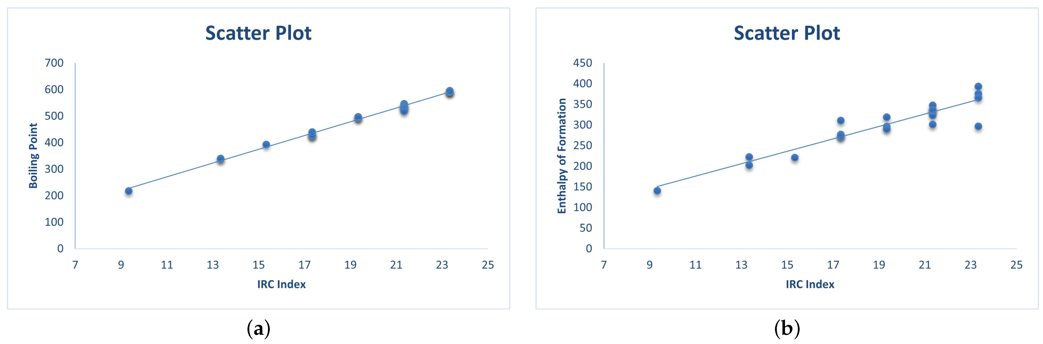
3.2. QSAR Modeling of Physicochemical Properties

Following a seminal work by Gutman et al. [39], in order to assess the efficiency of a topological descriptor, we choose two basic physicochemical properties known as the standard enthalpy of formation Δ H f o and the normal boiling point T b p . For the chemistry of the underlying chemical compounds, the enthalpy of formation exhibits the behavior of thermal properties, and the boiling point is supposed to constitute intermolecular and van der Waals interactions. The criterion to determine the performance of an irregularity index is simply the determination of the statistical correlation coefficient. The higher the value of the correlation coefficient is (i.e., closer to zero), the better the efficiency of the irregularity index.
Following the standard choice of chemical compounds, we regard lower benzenoid hydrocarbons, as they are supposed to represent both cyclic and acyclic chemical structures. For the sake of authenticity and reliability of the statistical inference, we use 22 lower benzenoid hydrocarbons. Public availability of experimental data is another considerable reason for choosing lower benzenoid hydrocarbons. Figure 1 depicts the 22 lower benzenoid hydrocarbons.
Experimental data of T b p for the lower PAHs considered here have been provided by the standard NIST databases [40]. On the other hand, the experimental data for Δ H f o have been retrieved from Allison and Burgess [2]. For tallying the data, we confirmed it with Nikolić et al. [41].
For the molecular graphs in Figure 1, we first employ the computational method in Section 3.1 to compute their I R C indices. Then, we conduct a detailed statistical analysis of the I R C index with the experimental data of T b p and Δ H f o for the PAHs in Figure 1. Corresponding statistical parameters, such as the correlation coefficient, the regression model with confidence interval, the standard error of fit, the determination coefficient, scatter plot, and so on, are computed to assess how closely the I R C index correlates with the experimental data. Table 1 exhibits the values of T b p , Δ H f o and the I R C indices of the 22 lower PAH graphs in Figure 1.
Let ρ be the correlation coefficient. Then, ρ ( Δ H f o ) and ρ ( T b p ) are presented in the following expression.
ρ ( T b p ) = 0.9967 , ρ ( Δ H f o ) = 0.9343 .
The corresponding linear regression models with 95 % confidence intervals for the slope and intercepts of the models, the determination coefficients, and the standard error of estimates are given as follows:
T b p = 25 . 937 ± 19.8399 I R C 13 . 847 ± 1.0223 , r 2 = 0.9933 , s = 8.3218 . Δ H f o = 15 . 003 ± 53.3614 I R C + 11 . 309 ± 2.7496 , r 2 = 0.8728 , s = 22.3824 .
Moreover, Figure 2 shows the scatter plot of two selected properties, that is, T b p and Δ H f o vs. IRC index.
The statistical analysis shows that the I R C index correlates well with the normal boiling point and fairly well with the enthalpy of formation for lower PAHs. Thus, based on the analysis in this section, we suggest that further applications of the I R C index in quantitative structure activity/property relationship models are warranted. This also suggests a window for exploring further mathematical properties of the I R C index.
Next, we derive some mathematical properties of the I R C index. First, we compute the I R C index of various transformation graphs introduced by Wu and Meng [34].

4. The IRC Indices of Transformation Graphs

First, we define some terminologies required later in this section. For a graph G, we define
ξ 4 ( G ) = u v E ( G ) d 3 ( u ) + d 3 ( v ) , χ α ( G ) = u v E ( G ) d ( u ) + d ( v ) α .
Next, we calculate the I R C indices of different transformation and total transformation graphs. The next theorem calculates the I R C index of G x y z , where x = y = z = + .
Theorem 1.
Let G be an ( n , e )-graph. Then, the I R C index of G + + + of G is
I R C ( G + + + ) = 8 F ( G ) + ξ 4 ( G ) + 3 R e Z G 3 ( G ) M 1 ( G ) + 4 e e + n 4 M 1 ( G ) + F ( G ) + 2 M 2 ( G ) .
Proof. 
By the definition of the I R C index, we have
I R C ( G ) = u V ( G ) d 3 ( u ) 2 e n u V ( G ) d 2 ( u ) .
Following the definition of the G + + + , we obtain
I R C ( G + + + ) = u V ( G + + + ) d 3 ( u ) 2 ( M 1 ( G ) 2 + 2 e ) e + n u V ( G + + + ) d 2 ( u ) .
By Lemma 2 and Equation (1), we obtain
I R C ( G + + + ) = u V x ( G + + + ) d 3 ( u ) + u V y ( G + + + ) d 3 ( u ) M 1 ( G ) + 4 e e + n u V x ( G + + + ) d 2 ( u ) + u V y ( G + + + ) d 2 ( u ) , = u V ( G ) 2 d ( u ) 3 + u v E ( G ) d ( u ) + d ( v ) 3 M 1 ( G ) + 4 e e + n 4 u V ( G ) 2 d ( u ) 2 + u v E ( G ) d ( u ) + d ( v ) 2 , = 8 F ( G ) + u v E ( G ) d 3 ( u ) + d 3 ( v ) + 3 u v E ( G ) d ( u ) d ( v ) d ( u ) + d ( v ) M 1 ( G ) + 4 e e + n 4 M 1 ( G ) + u v E ( G ) d 2 ( u ) + d 2 ( v ) + 2 u v E ( G ) d ( u ) d ( v ) , = 8 F ( G ) + ξ 4 ( G ) + 3 R e Z G 3 ( G ) M 1 ( G ) + 4 e e + n 4 M 1 ( G ) + F ( G ) + 2 M 2 ( G ) .
This implies that we obtain
I R C ( G + + + ) = 8 F ( G ) + ξ 4 ( G ) + 3 R e Z G 3 ( G ) M 1 ( G ) + 4 e e + n 4 M 1 ( G ) + F ( G ) + 2 M 2 ( G ) .
This completes the proof. □
The next theorem computes the I R C index of G x y z , where x = y = + , z = .
Theorem 2.
Let G be an ( n , e )-graph. Then, the I R C index of G + + of G is
I R C ( G + + ) = n m 3 + E F ( G ) + e ( n 2 ) 3 + 3 ( n 2 ) E M 1 ( G ) + 3 ( n 2 ) 2 ( M 1 ( G ) 2 e ) M 1 ( G ) + 2 e ( n 2 ) e + n n m 2 + E M 1 ( G ) + e ( n 2 ) 2 + 2 ( n 2 ) ( M 1 ( G ) 2 e ) .
Proof. 
Applying the definition of the I R C index, we have
I R C ( G ) = u V ( G ) d 3 ( u ) 2 e n u V ( G ) d 2 ( u ) .
Following the definition of the G + + , we obtain
I R C ( G + + ) = u V ( G + + ) d 3 ( u ) 2 ( M 1 ( G ) 2 + e ( n 2 ) ) e + n u V ( G + + ) d 2 ( u ) .
By Lemma 2 and Equation (1), we obtain
I R C ( G + + ) = u V x ( G + + ) d 3 ( u ) + u V y ( G + + ) d 3 ( u ) M 1 ( G ) + 2 e ( n 2 ) e + n u V x ( G + + ) d 2 ( u ) + u V y ( G + + ) d 2 ( u ) .
I R C ( G + + ) = u V ( G ) e 3 + f E ( G ) d ( f ) + n 2 3 M 1 ( G ) + 2 e ( n 2 ) e + n u V ( G ) e 2 + f E ( G ) d ( f ) + n 2 2 , = n m 3 + f E ( G ) d 3 ( f ) + f E ( G ) ( n 2 ) 3 + 3 ( n 2 ) f E ( G ) d ( f ) 2 + 3 ( n 2 ) 2 f E ( G ) d ( f ) M 1 ( G ) + 2 e ( n 2 ) e + n n m 2 + f E ( G ) d ( f ) + n 2 2 , = n m 3 + E F ( G ) + e ( n 2 ) 3 + 3 ( n 2 ) E M 1 ( G ) + 3 ( n 2 ) 2 ( M 1 ( G ) 2 e ) M 1 ( G ) + 2 e ( n 2 ) e + n n m 2 + f E ( G ) ( d ( f ) ) 2 + u v E ( G ) ( n 2 ) 2 + 2 ( n 2 ) f E ( G ) d ( f ) , = n m 3 + E F ( G ) + e ( n 2 ) 3 + 3 ( n 2 ) E M 1 ( G ) + 3 ( n 2 ) 2 ( M 1 ( G ) 2 e ) M 1 ( G ) + 2 e ( n 2 ) e + n n m 2 + E M 1 ( G ) + e ( n 2 ) 2 + 2 ( n 2 ) ( M 1 ( G ) 2 e ) .
Thus, we obtain
I R C ( G + + ) = n m 3 + E F ( G ) + e ( n 2 ) 3 + 3 ( n 2 ) E M 1 ( G ) + 3 ( n 2 ) 2 ( M 1 ( G ) 2 e ) M 1 ( G ) + 2 e ( n 2 ) e + n n m 2 + E M 1 ( G ) + e ( n 2 ) 2 + 2 ( n 2 ) ( M 1 ( G ) 2 e ) .
This completes the proof. □
The proofs of the remaining results in this section have structural similarities with the proofs of Theorems 1 and 2; therefore, we omit the remaining proofs. The following calculates the I R C index of G x y z , where x = + , y = z = .
Theorem 3.
Let G be an ( n , e )-graph. Then, the I R C index of G + of G is
I R C ( G + ) = n m 3 χ 3 ( G ) + e ( e + n 1 ) 3 + 3 ( e + n 1 ) χ 2 ( G ) 3 ( e + n 1 ) 2 M 1 ( G ) e 2 + 2 m n e M 1 ( G ) e + n n m 2 + e ( e + n 1 ) 2 + χ 2 ( G ) 2 ( e + n 1 ) M 1 ( G ) .
Next we calculate the I R C index of G x y z , where x = z = + , y = .
Theorem 4.
Let G be an ( n , e )-graph. Then, the I R C index of G + + of G is
I R C ( G + + ) = 8 F ( G ) χ 3 ( G ) + e ( e + 3 ) 3 + 3 ( e + 3 ) χ 2 ( G ) 3 ( e + 3 ) 2 M 1 ( G ) e 2 + 7 e M 1 ( G ) e + n 4 M 1 ( G ) + e ( e + 3 ) 2 + χ 2 ( G ) 2 ( e + 3 ) M 1 ( G ) .
Here, we calculate the I R C index of G x y z , where x = , y = z = + .
Theorem 5.
Let G be an ( n , e )-graph. Then, the I R C index of G + + of G is
I R C ( G + + ) = n ( n 1 ) 3 + χ 3 ( G ) M 1 ( G ) + n ( n 1 ) e + n n ( n 1 ) 2 + χ 2 ( G ) .
The next theorem computes the I R C index of G x y z , where x = y = , z = + .
Theorem 6.
Let G be an ( n , e )-graph. Then, the I R C index of G + of G is
I R C ( G + ) = n ( n 1 ) 3 χ 3 ( G ) + e ( e + 3 ) 3 + 3 ( e + 3 ) χ 2 ( G ) 3 ( e + 3 ) 2 M 1 ( G ) e 2 + n ( n 1 ) + 3 e M 1 ( G ) e + n n ( n 1 ) 2 + e ( e + 3 ) 2 + χ 2 ( G ) 2 ( e + 3 ) M 1 ( G ) .
Next, we find the I R C index of G x y z , where x = y = z = .
Theorem 7.
Let G be an ( n , e )-graph. Then, the I R C index of G of G is
I R C ( G ) = n ( e + n 1 ) 3 8 F ( G ) + 12 ( e + n 1 ) M 1 ( G ) 12 ( e + n 1 ) 2 e + e ( e + n 1 ) 3 χ 3 ( G ) + 3 ( e + n 1 ) χ 2 ( G ) 3 ( e + n 1 ) 2 M 1 ( G ) β ( n ( e + n 1 ) 2 β 4 M 1 ( G ) 8 e ( e + n 1 ) + e ( e + n 1 ) 2 + χ 2 ( G ) 2 ( e + n 1 ) M 1 ( G ) ,
where β = ( e + n ) 2 5 e n M 1 ( G ) e + n .
Finally, we calculate the I R C index of G x y z , where x = z = , y = + .
Theorem 8.
Let G be an ( n , e )-graph. Then, the I R C index of G + of G is
I R C ( G + ) = n ( e + n 1 ) 3 8 F ( G ) + 12 ( e + n 1 ) M 1 ( G ) 12 ( e + n 1 ) 2 e + e ( n 1 ) 3 + χ 3 ( G ) + 3 ( n 1 ) χ 2 ( G ) + 3 ( n 1 ) 2 M 1 ( G ) β ( n ( e + n 1 ) 2 β 4 M 1 ( G ) 8 e ( e + n 1 ) + e ( n 1 ) 2 + χ 2 ( G ) + 2 ( n 1 ) M 1 ( G ) ,
where β = M 1 ( G ) + 2 e ( n 4 ) + n ( n 1 ) e + n .
The next section calculates analytically closed formulas of the I R C for various derived graphs introduced in Section 2.

5. The IRC Indices of Derived Graphs

This section calculates the I R C indices of various derived graphs, including the subdivision graph, the line graph, the semi-total point graph, the semi-total line graph, the total graph, the double graph, the strong double graph, and the extended double cover graph.
Next, we calculate the I R C index of the subdivision graph.
Theorem 9.
Let G be an ( n , e )-graph. Then, the I R C index of the subdivision graph S ( G ) of G is
I R C ( S ( G ) = F ( G ) + 8 e 4 m M 1 ( G ) e + n 8 e 2 e + n .
Proof. 
By definition of the I R C index, we have
I R C ( G ) = u V ( G ) d 3 ( u ) 2 e n u V ( G ) d 2 ( u ) .
By definition of the subdivision graph, we have
V L ( G ) = n + e , E L ( G ) = 2 e .
Employing this for I R C ( G ) , we obtain
I R C ( S ( G ) ) = u V ( S ( G ) ) d 3 ( u ) 2 e n u V ( S ( G ) ) d 2 ( u ) .
By Lemma 1, we obtain
I R C ( S ( G ) ) = u V ( G ) d 3 ( u ) + u E ( G ) 2 3 2 e n u V ( G ) d 2 ( u ) + u E ( G ) 2 2 , = F ( G ) + 8 e 2 e n M 1 ( G ) + 4 e , = F ( G ) + 8 e 2 e n M 1 ( G ) 8 e 2 n .
Thus, we have
I R C ( S ( G ) ) = F ( G ) + 8 e 2 e n M 1 ( G ) 8 e 2 n .
This completes the proof. □
The following theorem computes the I R C index of the line graph.
Theorem 10.
Let G be an ( n , e )-graph. Then, the I R C index of the line graph L ( G ) of G is
I R C ( L ( G ) ) = E F ( G ) M 1 ( G ) 2 e e E M 1 ( G ) .
Proof. 
By definition of the I R C index, we have
I R C ( G ) = u V ( G ) d 3 ( u ) 2 e n u V ( G ) d 2 ( u ) .
By definition of the line graph, we have
V ( L ( G ) ) = e , E L ( G ) = M 1 ( G ) 2 e .
Using this information for I R C ( G ) , we obtain
I R C ( L ( G ) ) = u V ( L ( G ) ) d 3 ( u ) 2 ( M 1 ( G ) 2 e ) e u V ( L ( G ) ) d 2 ( u ) .
By Lemma 1, we obtain
I R C ( L ( G ) ) = f E ( G ) d 3 ( f ) M 1 ( G ) 2 e e f E ( G ) d 2 ( f ) , = E F ( G ) M 1 ( G ) 2 e e E M 1 ( G ) .
Therefore, we obtain
I R C ( S ( G ) ) = E F ( G ) M 1 ( G ) 2 e e E M 1 ( G ) .
This completes the proof. □
Next, we calculate the exact expression of the the I R C index of the semi-total point graph.
Theorem 11.
Let G be an ( n , e )-graph. Then, the I R C index of the semi-total point graph T 1 ( G ) of G is
I R C T 1 ( G ) = 8 F ( G ) + 8 e 24 e n + e M 1 ( G ) e .
Proof. 
By definition of the I R C index, we have
I R C ( G ) = u V ( G ) d 3 ( u ) 2 e n u V ( G ) d 2 ( u ) .
By definition of the semi-total point graph, we have
V T 1 ( G ) = n + e , E T 1 ( G ) = 3 e .
Using this information for I R C ( G ) , we obtain
I R C T 1 ( G ) = u V ( S ( G ) ) d 3 ( u ) 2 · 3 e n + e u V ( S ( G ) ) d 2 ( u ) .
By Lemma 1, we obtain
I R C T 1 ( G ) = u V ( G ) ( 2 d ( u ) ) 3 + u E ( G ) 2 3 6 e n + e ( u V ( G ) ( 2 d ( u ) ) 2 + u E ( G ) 2 2 ) , = 8 F ( G ) + 8 e 6 e n + e ( 4 M 1 ( G ) + 4 e ) , = 8 F ( G ) + 8 e 24 e n + e M 1 ( G ) 24 e 2 n + e .
This shows that
I R C ( G 1 ( G ) ) = 8 F ( G ) + 8 e 24 e n + e M 1 ( G ) e .
This completes the proof. □
The next theorem calculates the the I R C index of the semi-total line graph.
Theorem 12.
Let G be an ( n , e )-graph. Then, the I R C index of the semi-total line graph T 2 ( G ) of G is
I R C T 2 ( G ) = F ( G ) + χ 3 ( G ) 2 e + M 1 ( G ) n + e M 1 ( G ) + F ( G ) + 2 M 2 ( G ) .
Proof. 
By definition of the I R C index, we have
I R C ( G ) = u V ( G ) d 3 ( u ) 2 e n u V ( G ) d 2 ( u ) .
By definition of the semi-total line graph, we have
V T 2 ( G ) = n + e , E T 2 ( G ) = e + M 1 ( G ) 2 .
Using this information for I R C ( G ) , we obtain
I R C T 2 ( G ) = u V T 2 ( G ) d 3 ( u ) 2 ( e + M 1 ( G ) 2 ) n + e u V T 2 ( G ) d 2 ( u ) .
By Lemma 1, we obtain
I R C T 2 ( G ) = u V ( G ) ( d 3 ( u ) ) + v = v 1 v 2 E ( G ) d ( v 1 ) + d ( v 2 ) 3 2 e + M 1 ( G ) n + e u V T 2 ( G ) d 2 ( u ) , = F ( G ) + χ 3 ( G ) 2 e + M 1 ( G ) n + e u V ( G ) d 2 ( u ) + v = v 1 v 2 E ( G ) d ( v 1 ) + d ( v 2 ) 2 , = F ( G ) + χ 3 ( G ) 2 e + M 1 ( G ) n + e M 1 ( G ) + F ( G ) + 2 M 2 ( G ) .
Thus, we have
I R C ( G 2 ( G ) ) = 3 F ( G ) + 3 M 1 ( G ) M 2 ( G ) 2 e + M 1 ( G ) n + e ( M 1 ( G ) + F ( G ) + 2 M 2 ( G ) ) .
This completes the proof. □
The following theorem calculates the the I R C index of the total graph.
Theorem 13.
Let G be an ( n , e )-graph. Then, the I R C index of the total graph T ( G ) of G is
I R C T ( G ) = 8 F ( G ) + χ 3 ( G ) 4 e + M 1 ( G ) n + e 4 M 1 ( G ) + F ( G ) + 2 M 2 ( G ) .
Proof. 
By definition of the I R C index, we have
I R C ( G ) = u V ( G ) d 3 ( u ) 2 e n u V ( G ) d 2 ( u ) .
By definition of the total graph, we have
V T ( G ) = n + e , E T ( G ) = 2 e + M 1 ( G ) 2 .
Using this information for I R C ( G ) , we obtain
I R C T ( G ) = u V T ( G ) d 3 ( u ) 2 2 e + M 1 ( G ) 2 n + e u V T ( G ) d 2 ( u ) .
By Lemma 1, we obtain
I R C T ( G ) = u V ( G ) 2 d ( u ) 3 + v = v 1 v 2 E ( G ) d ( v 1 ) + d ( v 2 ) 3 4 e + M 1 ( G ) n + e u V T ( G ) d 2 ( u ) , = 8 F ( G ) + χ 3 ( G ) 4 e + M 1 ( G ) n + e u V ( G ) 2 d ( u ) 2 + v = v 1 v 2 E ( G ) d ( v 1 ) + d ( v 2 ) 2 , = 8 F ( G ) + χ 3 ( G ) 4 e + M 1 ( G ) n + e u V ( G ) 2 d ( u ) 2 + v = v 1 v 2 E ( G ) d ( v 1 ) + d ( v 2 ) 2 , = 8 F ( G ) + χ 3 ( G ) 4 e + M 1 ( G ) n + e 4 M 1 ( G ) + F ( G ) + 2 M 2 ( G ) .
Thus, we obtain
I R C ( T ( G ) ) = 10 F ( G ) + 3 M 1 ( G ) M 2 ( G ) 4 e + M 1 ( G ) n + e ( 4 M 1 ( G ) + F ( G ) + 2 M 2 ( G ) ) .
This completes the proof. □
Next, we calculate the exact expression of the the I R C index of the double graph.
Theorem 14.
Let G be an ( n , e )-graph. Then, the I R C index of the double graph D ( G ) of G is
I R C D ( G ) = 16 F ( G ) 32 m M 1 ( G ) n .
Proof. 
By definition of the I R C index, we have
I R C ( G ) = u V ( G ) d 3 ( u ) 2 e n u V ( G ) d 2 ( u ) .
By definition of the double graph, we have
I R C D ( G ) = u V D ( G ) d 3 ( u ) 2 × 4 e 2 n u V D ( G ) d 2 ( u ) = 2 u V ( G ) 2 d ( u ) 3 4 e n 2 u V ( G ) 2 d ( u ) 2 , = 16 F ( G ) 4 e n 8 M 1 ( G ) , = 16 F ( G ) 32 e n M 1 ( G ) .
Thus, we obtain
I R C ( D ( G ) ) = 16 F ( G ) 32 e n M 1 ( G ) .
This completes the proof. □
The following theorem computes the I R C index of the strong double graph.
Theorem 15.
Let G be an ( n , e )-graph. Then, the I R C index of the strong double graph S D ( G ) of G is
I R C S D ( G ) = 16 F ( G ) + 2 n + 24 M 1 ( G ) M 2 ( G ) + 24 e 5 e n 8 M 1 ( G ) + 2 n + 16 e .
Proof. 
By definition of the I R C index, we have
I R C ( G ) = u V ( G ) d 3 ( u ) 2 e n u V ( G ) d 2 ( u ) .
By definition of the strong double graph, we have
I R C ( S D ( G ) ) = u V S D ( G ) d 3 ( u ) 2 × 5 e 2 n u V S D ( G ) d 2 ( u ) = 2 u V ( G ) 2 d ( u ) + 1 3 5 e n ( 2 u V ( G ) 2 d ( u ) + 1 2 = 2 8 F ( G ) + n + 12 M 1 ( G ) + 12 e 5 e n 2 4 M 1 ( G ) + n + 8 e = 16 F ( G ) + 2 n + 24 M 1 ( G ) + 24 e 5 e n 8 M 1 ( G ) + 2 n + 16 e .
Thus, we have
I R C S D ( G ) = 16 F ( G ) + 2 n + 24 M 1 ( G ) + 24 e 5 e n ( 8 M 1 ( G ) + 2 n + 16 e ) .
This completes the proof. □
The next theorem calculates the I R C index of the extended double cover graph.
Theorem 16.
Let G be an ( n , e )-graph. Then, the I R C index of the extended double cover graph G * of G is
I R C ( G * ) = 2 F ( G ) + 2 n + 6 M 1 ( G ) M 2 ( G ) + 12 e 3 e n ( 2 M 1 ( G ) + 2 n + 8 e ) .
Proof. 
By definition of the I R C index, we have
I R C ( G ) = u V ( G ) d 3 ( u ) 2 e n u V ( G ) d 2 ( u )
By definition of the extended double cover graph, we have
I R C ( G * ) = u V ( G * ) d 3 ( u ) 2 · 3 e 2 n u V ( G * ) d 2 ( u ) = 2 u V ( G ) ( d ( u ) + 1 ) 3 3 e n ( 2 u V ( G ) ( d ( u ) + 1 ) 2 = 2 F ( G ) + n + 3 M 1 ( G ) + 6 e 3 e n 2 M 1 ( G ) + n + 4 e = 2 F ( G ) + 2 n + 6 M 1 ( G ) + 12 e 3 e n 2 M 1 ( G ) + 2 n + 8 e .
Thus, we have
I R C ( G ) = 2 F ( G ) + 2 n + 6 M 1 ( G ) + 12 e 3 e n ( 2 M 1 ( G ) + 2 n + 8 e ) .
This completes the proof. □

6. Conclusions

This paper employs a recently introduced irregularity index (i.e., the I R C index) in QSAR modeling of physicochemical properties of chemical compounds. The results show that the I R C index correlates closely with certain physicochemical properties of benzenoid hydrocarbons. A detailed statistical analysis has been conducted to propose appropriate regression models, which in our case are linear. Considering this as a motivation to study the I R C index further, we calculate the I R C indices for various transformation and derived graphs. Moreover, further mathematical investigation of this I R C index is proposed herein.

Author Contributions

H.L. and S.H. contributed equally to this work. Conceptualization, H.L. and S.H.; methodology, H.L. and S.H.; software, Z.P.; validation, H.L., Z.P. and Y.Z.; formal analysis, T.R.; investigation, H.L. and S.H.; resources, Z.P..; data curation, H.L. and Z.P.; writing—original draft preparation, H.L., S.H. and Z.P.; writing—review and editing, Z.P. and T.R.; visualization, S.H.; supervision, Y.Z.; project administration, T.R.; funding acquisition, Z.P. All authors have read and agreed to the published version of the manuscript.

Funding

This research received no external funding.

Institutional Review Board Statement

Not applicable.

Informed Consent Statement

Not applicable.

Data Availability Statement

There is no data associated with this manuscript.

Conflicts of Interest

The authors declare no conflict of interest.

References

  1. Roy, K.; Kar, S.; Das, R.N. A Primer on QSAR/QSPR Modeling: Fundamental Concepts; Springer: Berlin/Heidelberg, Germany, 2015. [Google Scholar]
  2. Allison, T.C.; Burgess, D.R., Jr. First-principles prediction of enthalpies of formation for polycyclic aromatic hydrocarbons and derivatives. J. Phys. Chem. A 2015, 119, 11329–11365. [Google Scholar] [CrossRef] [Green Version]
  3. Estrada, E.; Torres, L.; Rodríguez, L.; Gutman, I. An atom-bond connectivity index: Modelling the enthalpy of formation of alkanes. Indian J. Chem. 1998, 37A, 849–855. [Google Scholar]
  4. Redžepović, I.; Marković, S.; Furtula, B. On structural dependence of enthalpy of formation of catacondensed benzenoid hydrocarbons. MATCH Commun. Math. Comput. Chem. 2019, 82, 663–678. [Google Scholar]
  5. Yu, J.; Sumathi, R.; Green, W.H. Accurate and efficient method for predicting thermochemistry of polycyclic aromatic hydrocarbons-bond-centered group additivity. J. Am. Chem. Soc. 2004, 126, 12685–12700. [Google Scholar] [CrossRef] [PubMed]
  6. Zavitsas, A.A.; Matsunaga, N.; Rogers, D.W. Enthalpies of formation of hydrocarbons by hydrogen atom counting. Theoretical implications. J. Phys. Chem. A 2008, 112, 5734–5741. [Google Scholar] [CrossRef] [PubMed]
  7. Teixeira, A.L.; Leal, J.P.; Falcao, A.O. Random forests for feature selection in QSPR models–an application for predicting standard enthalpy of formation of hydrocarbons. J. Cheminf. 2013, 5, 9–24. [Google Scholar] [CrossRef]
  8. Song, X.; Chai, L.; Zhang, J. Graph signal processing approach to QSAR/QSPR model learning of compounds. IEEE Trans. Pattern Anal. Mach. Intell. 2020, in press. [Google Scholar] [CrossRef]
  9. Dudek, A.Z.; Arodz, T.; Galvez, J. Computational methods in developing quantitative structure-activity relationships (QSAR): A review. Comb. Chem. High Throughput Screen. 2006, 9, 213–228. [Google Scholar] [CrossRef] [PubMed]
  10. Mauri, A.; Consonni, V.; Todeschini, R. Molecular Descriptors. Handbook of Computational Chemistry; Springer: Cham, Switzerland, 2016. [Google Scholar]
  11. Todeschini, R.; Consonni, V. Molecular Descriptors for Chemoinformatics; Wiley-VCHL: Weinheim, Germany, 2009; Volume 1–2. [Google Scholar]
  12. Dearden, J.C. Advances in QSAR Modeling-Applications in Pharmaceutical, Chemical, Food, Agricultural and Environmental Sciences; Roy, K., Ed.; Springer: Cham, Switzerland, 2017. [Google Scholar]
  13. Devillers, J.; Balaban, A.T. Topological Indices and Related Descriptors in QSAR and QSPR; Gordon & Breach: Amsterdam, The Netherlands, 1999. [Google Scholar]
  14. Talevi, A.; Bellera, C.L.; Di Ianni, M.; Duchowicz, P.R.; Bruno-Blanch, L.E.; Castro, E.A. An integrated drug development approach applying topological descriptors. Curr. Comput. Aided Drug Des. 2012, 8, 172–181. [Google Scholar] [CrossRef] [PubMed]
  15. Réti, T.; Sharafdini, R.; Dregelyi-Kiss, A.; Haghbin, H. Graph irregularity indices used as molecular descriptor in QSPR studies. MATCH Commun. Math. Comput. Chem. 2018, 79, 509–524. [Google Scholar]
  16. Ascioglu, M.; Cangul, I.N. Sigma index and forgotten index of the subdivision and r-subdivision graphs. Proc. Jangjeon Math. 2018, 21, 375–383. [Google Scholar]
  17. Réti, T. On some properties of graph irregularity indices with a particular regard to the σ-index. Appl. Math. Comput. 2019, 344–345, 107–115. [Google Scholar] [CrossRef]
  18. Diudea, M.V.; Gutman, I.; Lorentz, J. Molecular Topology; Nova Science Publishers: New York, NY, USA, 2001. [Google Scholar]
  19. Collatz, L.; Sinogowitz, U. Spektren endlicher grafen. Abh. Math. Sem. Univ. Hamburg. 1957, 21, 63–77. [Google Scholar] [CrossRef]
  20. Bell, F.K. A note on the irregularity of a graph. Linear Algebra Appl. 1992, 161, 45–54. [Google Scholar] [CrossRef] [Green Version]
  21. Gutman, I.; Togan, M.; Yurttas, A.; Cevik, A.S.; Cangul, I.N. Inverse problem for sigma index. MATCH Commun. Math. Comput. Chem. 2018, 79, 491–508. [Google Scholar]
  22. Gutman, I.; Trinajstić, N. Graph theory and molecular orbitals: Total π-electron energy of alternant hydrocarbons. Chem. Phys. Lett. 1972, 17, 535–538. [Google Scholar] [CrossRef]
  23. Gutman, I.; Das, K.C. The first Zagreb index 30 years after. MATCH Commun. Math. Comput. Chem. 2004, 50, 83–92. [Google Scholar]
  24. Gutman, I. Degree-based topological indices. Croat. Chem. Acta 2013, 86, 351–361. [Google Scholar] [CrossRef]
  25. Furtula, A.; Gutman, I. A forgotten topological index. J. Math. Chem. 2015, 53, 1184–1190. [Google Scholar] [CrossRef]
  26. Réti, T.; Toth-Laufer, E. On the construction and comparison of graph irregularity indices. Kragujevac J. Sci. 2017, 39, 53–75. [Google Scholar] [CrossRef] [Green Version]
  27. Cioabă, S.M. Sums of powers of the degrees of a graph. Discrete Math. 2006, 306, 1959–1964. [Google Scholar] [CrossRef] [Green Version]
  28. Ilić, A.; Zhou, B. On reformulated Zagreb indices. Discret. Appl. Math. 2012, 160, 204–209. [Google Scholar] [CrossRef] [Green Version]
  29. Ranjini, P.S.; Lokesha, V.; Usha, A. Relation between phenylene and hexagonal squeeze using harmonic index. Int. J. Graph Theory 2013, 1, 116–121. [Google Scholar]
  30. Behzad, M. A criterion for the planarity of a total graph. Proc. Cambridge Philos. Soc. 1967, 63, 679–681. [Google Scholar] [CrossRef]
  31. Sampathkumar, E.; Chikkodimath, S.B. The semi-total graphs of a graph-I. J. Karnatak Univ.-Sci. 1973, 18, 274–280. [Google Scholar]
  32. Akiyama, J.; Hamada, T.; Yoshimura, I. Miscellaneous properties of middle graphs. TRU Math. 1974, 10, 41–53. [Google Scholar]
  33. Alon, N. Eigenvalues and expanders. Combinatorica 1986, 6, 83–89. [Google Scholar] [CrossRef]
  34. Wu, B.; Meng, J. Basic properties of total transformation graphs. J. Math. Study 2001, 34, 109–116. [Google Scholar]
  35. Xu, L.; Wu, B. Transformation graph G−+−. Discrete Math. 2008, 308, 5144–5148. [Google Scholar] [CrossRef] [Green Version]
  36. Yi, L.; Wu, B. The transformation graph G++−. Aust. J. Comb. 2009, 44, 37–42. [Google Scholar]
  37. Stevanović, D.; Brankov, V.; Cvetković, D.; Simić, S. newGRAPH: A Fully Integrated Environment used for Research Process in Graph Theory. Available online: http://www.mi.sanu.ac.rs/newgraph/index.html (accessed on 21 February 2022).
  38. MATLAB 8.0 and Statistics Toolbox 8.1; The MathWorks, Inc.: Natick, MA, USA, 2022.
  39. Gutman, I.; Tošović, J. Testing the quality of molecular structure descriptors. Vertex-degree-based topological indices. J. Serb. Chem. Soc. 2013, 78, 805–810. [Google Scholar] [CrossRef]
  40. NIST Standard Reference Database. Available online: http://webbook.nist.gov/chemistry/ (accessed on 21 February 2022).
  41. Nikolić, S.; Trinajstić, N.; Baučić, I. Comparison between the vertex- and edge-connectivity indices for benzenoid hydrocarbons. J. Chem. Inf. Comput. Sci. 1998, 38, 42–46. [Google Scholar] [CrossRef]
Figure 1. The 22 lower benzenoid hydrocarbon graphs.
Mathematics 10 01111 g001aMathematics 10 01111 g001b
Figure 2. Scatter plots between the I R C index and the two selected properties (i.e., T b p and Δ H f o ). (a) A scatter plot between I R C and T b p . (b) A scatter plot between I R C and Δ H f o .
Mathematics 10 01111 g002
Table 1. The experimental data of T b p , Δ H f o , and the I R C index of the 22 lower PAHs.
Molecule T bp in °C Δ H f o in kJ/mol IRC
Benzene80.175.20
Naphthalene2181419.3333
Phenanthrene338202.713.3333
Anthracene340222.613.3333
Chrysene431271.117.3333
Benzo[a]anthracene425277.117.3333
Triphenylene429275.117.3333
Tetracene440310.517.3333
Benzo[a]pyrene49629619.3333
Benzo[e]pyrene493289.919.3333
Perylene497319.219.3333
Anthanthrene54732321.3333
Benzo[ghi]perylene542301.221.3333
Dibenzo[a,c]anthracene53534821.3333
Dibenzo[a,h]anthracene53533521.3333
Dibenzo[a,j]anthracene531336.321.3333
Picene519336.921.3333
Coronene590296.723.3333
Dibenzo(a,h)pyrene596375.623.3333
Dibenzo(a,i)pyrene59436623.3333
Dibenzo(a,l)pyrene595393.323.3333
Pyrene393221.315.3333
Publisher’s Note: MDPI stays neutral with regard to jurisdictional claims in published maps and institutional affiliations.

