Certain New Models of the Multi-Space Fractal-Fractional Kuramoto-Sivashinsky and Korteweg-de Vries Equations

Abstract

The main objective of this paper is to introduce and study the numerical solutions of the multi-space fractal-fractional Kuramoto-Sivashinsky equation (MSFFKS) and the multi-space fractal-fractional Korteweg-de Vries equation (MSFFKDV). These models are obtained by replacing the classical derivative by the fractal-fractional derivative based upon the generalized Mittag-Leffler kernel. In our investigation, we use the spectral collocation method (SCM) involving the shifted Legendre polynomials (SLPs) in order to reduce the new models to a system of algebraic equations. We then use one of the known numerical methods, the Newton-Raphson method (NRM), for solving the resulting system of the nonlinear algebraic equations. The efficiency and accuracy of the numerical results are validated by calculating the absolute error as well as the residual error. We also present several illustrative examples and graphical representations for the various results which we have derived in this paper.

1. Introduction

Many researchers have been attracted to study the behavior of solutions for many mathematical models, which are closely related to the real-world problems in (for example) biological, chemical and physical sciences, as well as in economic models (see, for example [1,2,3,4,5,6,7,8]). For most of these models, it is difficult to find the exact analytical solutions to them. This difficulty is among the many challenges facing researchers in the applied sciences (see, for example [9,10]). Hence, this challenge has attracted many researchers to this field, who are in search of appropriate numerical methods to find approximate and numerical solutions for these models (see [11,12]). In the existing literature, one can find simulations which were made by means of such familiar computer programs such as Mathematica, Matlab, Maple, and others. This procedure, in fact, has become remarkably useful for researchers in such applied scientific fields as biology, chemistry, physics and economics (see, for example [13,14,15]). Thus, by using these models and numerical solutions together with computer simulations, it is possible to simulate many laboratory experiments.

Our presentation in this article is organized as follows. In Section 2, the basic definitions and main theory are presented. In Section 3, a method based upon, and the relevant properties of, the familiar Legendre polynomials are presented and also the scheme of the two equations are considered. In Section 4, the numerical results are studied and a convincingly good agreement is found. Finally, in Section 5, we include some remarks and observations.

2. Basic Definitions and the Main Theorems

We first define the one-parameter Mittag-Leffler function $E_{\beta }\left(\xi \right)$.

Definition 1.

The Mittag-Leffler function $E_{\beta }\left(\xi \right)$ of the parameter β is given by

$$\begin{array}{c}\hfill E_{\beta }\left(\xi \right)=\sum _{k=0}^{\infty }\frac{{\xi }^k}{\mathsf{\Gamma }(\beta k+1)}(\xi \in \mathbb{R};\beta >0),\end{array}$$

(1)

and

$$\begin{array}{c}\hfill E_{\beta ,\alpha }\left(\xi \right)=\sum _{k=0}^{\infty }\frac{{\xi }^k}{\mathsf{\Gamma }(\beta k+\alpha )}(\xi \in \mathbb{R};\beta ,\alpha >0).\end{array}$$

(2)

Based on the definitions in [16,17,18], we can introduce the following definitions.

Definition 2.

Let $\psi \in H^1(a,b)(a<b)$ and $\beta ,r\in (0,1)$. Then the fractal-fractional derivative of order $(\beta ,r)$ of the continuous function $\psi \left(\xi \right)$ via the Mittag-Leffler kernel in the left-sided Riemann-Liouville sense is given by

$$\begin{array}{c}\hfill \left({}_a^{\mathrm{FFM}}{D}_r^{\beta }\psi \right)\left(\xi \right)=\frac{M\left(\beta \right)}{1-\beta }\frac{d}{d{\xi }^r}{\int }_a^{\xi }\psi \left(\tau \right)E_{\beta }\left(-\beta \frac{{(\xi -\tau )}^{\beta }}{1-\beta }\right)d\tau .\end{array}$$

(3)

We now define the higher-order fractal-fractional derivative as follows.

Definition 3.

The fractal-fractional derivative of order $(\nu ,r)$ of the continuous function $\psi \left(\xi \right)$ via the Mittag-Leffler kernel in the left-sided Riemann-Liouville sense, denoted by ${}_a^{\mathrm{FFM}}{D}_r^{\nu }$, is given by

$${}_a^{\mathrm{FFM}}{D}_r^{\nu }\psi \left(x\right)=\frac{M\left(\beta \right)}{1-\beta }\frac{d}{d{\xi }^r}{\int }_a^{\xi }{\psi }^{(n+1)}\left(\tau \right)E_{\beta }\left(-\beta \frac{{(\xi -\tau )}^{\beta }}{1-\beta }\right)d\tau$$

(4)

$$(n<\nu \leqq n+1;0<r<1)$$

or, equivalently,

$${}_a^{\mathrm{FFM}}{D}_r^{\nu }\psi \left(x\right)=\frac{M\left(\beta \right){\xi }^{1-r}}{(1-\beta )r}\frac{d}{d\xi }{\int }_a^{\xi }{\psi }^{(n+1)}\left(\tau \right)E_{\beta }\left(-\beta \frac{{(\xi -\tau )}^{\beta }}{1-\beta }\right)d\tau$$

(5)

$$(n<\nu \leqq n+1;0<r<1).$$

In Definitions 1 and 2 above, we have

$$\frac{d}{d{\eta }^r}\left\{\psi \left(\eta \right)\right\}=\underset{\tau \to \eta }{lim}\frac{\psi \left(\tau \right)-\psi \left(\eta \right)}{{\tau }^r-{\eta }^r}.$$

(6)

We also have $n=\lfloor \nu \rfloor$ (that is, the integer part of $\nu$), $\beta =\lceil \nu \rceil$ (that is, the decimal part of $\nu$) and $M\left(\beta \right)$ is the normalization function such that $M\left(0\right)=M\left(1\right)=1$,

Theorem 1.

The left-sided FFM of order $(\nu ,r),$ where $\nu \in (n,n+1]$ and $r\in (0,1),$ of the function $\psi \left(\xi \right)={\xi }^{\gamma }(\gamma >1;\gamma \geqq \lceil \nu \rceil )$ is given by

$$\begin{array}{cc}\hfill {}_a^{\mathrm{FFM}}{D}_r^{\nu }{\xi }^{\gamma }& =\frac{M\left(\beta \right)\mathsf{\Gamma }(\gamma +1){\xi }^{1-r}}{(1-\beta )r\mathsf{\Gamma }\left(\lambda \right)}\sum _{k=0}^{\infty }{\beta }^{\beta k}\left[a{\xi }^{\alpha -1}{\left(1-\frac{a}{\xi }\right)}^{\beta k}{\left(\frac{a}{\xi }\right)}^{\gamma -n}\right.\hfill \\ \hfill & \left.+(\alpha +1){\xi }^{\alpha }\left(\frac{\mathsf{\Gamma }\left(\lambda \right)\mathsf{\Gamma }(k\beta +1)}{\mathsf{\Gamma }(\alpha +2)}-B_{\frac{a}{\xi }}(\lambda ,k\beta +1)\right)\right],\hfill \end{array}$$

(7)

where $\alpha =\gamma +\beta k-n$ and $\lambda =\gamma -n+1$.

Proof. 

According to Equation (5), we have

$$\begin{array}{cc}\hfill {}_a^{\mathrm{FFM}}{D}_r^{\nu }{\xi }^{\gamma }& =\frac{M\left(\beta \right){\xi }^{1-r}}{(1-\beta )r}\frac{d}{d\xi }{\int }_a^{\xi }{D}^{(n+1)}{\tau }^{\gamma }{E}_{\beta }\left(-\frac{\beta {(\xi -\tau )}^{\beta }}{1-\beta }\right)d\tau \hfill \\ \hfill & =\frac{M\left(\beta \right)\mathsf{\Gamma }(\gamma +1){\xi }^{1-r}}{(1-\beta )r\mathsf{\Gamma }\left(\lambda \right)}\frac{d}{d\xi }{\int }_a^{\xi }{\tau }^{\gamma -n-1}\sum _{k=0}^{\infty }\frac{{\beta }^{\beta k}{(\xi -\tau )}^{\beta k}}{\mathsf{\Gamma }(k\beta +1)}d\tau \hfill \\ \hfill & =\frac{M\left(\beta \right)\mathsf{\Gamma }(\gamma +1){\xi }^{1-r}}{(1-\beta )r\mathsf{\Gamma }\left(\lambda \right)}\frac{d}{d\xi }\sum _{k=0}^{\infty }\frac{{\beta }^{\beta k}\left[{\xi }^{\alpha +1}\left(\frac{\mathsf{\Gamma }\left(\lambda \right)\mathsf{\Gamma }(k\beta +1)}{\mathsf{\Gamma }(\alpha +2)}-B_{\frac{a}{\xi }}(\lambda ,k\beta +1)\right)\right]}{\mathsf{\Gamma }(k\beta +1)}\hfill \\ \hfill & =\frac{M\left(\beta \right)\mathsf{\Gamma }(\gamma +1){\xi }^{1-r}}{(1-\beta )r\mathsf{\Gamma }\left(\lambda \right)}\sum _{k=0}^{\infty }{\beta }^{\beta k}\left[a{\xi }^{\alpha -1}{\left(1-\frac{a}{\xi }\right)}^{\beta k}{\left(\frac{a}{\xi }\right)}^{\gamma -n}\right.\hfill \\ \hfill & \left.+(\alpha +1){\xi }^{\alpha }\left(\frac{\mathsf{\Gamma }\left(\lambda \right)\mathsf{\Gamma }(k\beta +1)}{\mathsf{\Gamma }(\alpha +2)}-B_{\frac{a}{\xi }}(\lambda ,k\beta +1)\right)\right],\hfill \end{array}$$

which completes the proof of Theorem 1. □

Upon setting $r=0$ in Theorem 1, we obtain the result derived in [19]. Moreover, for $n=0$ and $a=0$, Theorem 1 yields the result given in [20].

3. Legendre Polynomials and Numerical Scheme

Orthogonal functions and spectral methods have attracted the interest of many researchers and have become an important performer for solving differential equations. Recently, these methods have also been employed in finding numerical solutions of fractional differential equations (see, for example [21,22]).

3.1. The Shifted Legendre Polynomials

We begin by defining the shifted Legendre polynomials on the interval $[0,1]$ with the variable $z=2\xi -1$. These polynomials possess the following property:

$${\varphi }_k\left(\xi \right)={\varphi }_k(2\xi -1)={\varphi }_{2k}\left(\sqrt{\xi }\right),$$

where the set ${\left\{{\varphi }_k\left(\xi \right)\right\}}_{k\in {\mathbb{N}}_0}$ forms a family of orthogonal Legendre polynomials on the interval $[-1,1]$ (see, for details [23]), ${\mathbb{N}}_0:=\mathbb{N}\cup \left\{0\right\}$ being the set of non-negative integers. The analytic form of the shifted Legendre polynomials of degree s is given by

$${\overline{\varphi }}_i\left(\xi \right)=\sum _{k=0}^i\frac{{(-1)}^{i+k}(i+k)!}{{(k!)}^2(i-k)!}{\xi }^k({\overline{\varphi }}_0\left(\xi \right)=1;{\overline{\varphi }}_1\left(\xi \right)=2\xi -1;i\in \mathbb{N}\backslash \left\{1\right\}).$$

(8)

The function $\psi \left(\xi \right)\in {\mathcal{L}}_2[0,1]$ can be expressed and approximated as a linear combination of the first $m+1$ terms of ${\overline{\varphi }}_i\left(\xi \right)$ as follows:

$$\psi \left(\xi \right)\simeq {\psi }_{\iota }\left(\xi \right)=\sum _{i=0}^{\iota }{\upsilon }_i{\overline{\varphi }}_i\left(\xi \right)(\iota \in \mathbb{N}),$$

(9)

where the coefficients ${\upsilon }_i$ are given by

$${\upsilon }_i=(2i+1){\int }_0^1\psi \left(\xi \right){\overline{\varphi }}_i\left(\xi \right)d\xi (i\in {\mathbb{N}}_0).$$

We now state and prove the main approximation formula of ${}_0^{\mathrm{FFM}}{D}^{\nu }{\psi }_{\iota }\left(\xi \right)$ as Theorem 2 below.

Theorem 2.

For the FFM-derivative operator ${}_0^{\mathrm{FFM}}{D}_r^{\nu }\left({\psi }_{\iota }\left(\xi \right)\right),$ it is asserted that

$${}_0^{\mathrm{FFM}}{D}_r^{\nu }\left({\psi }_{\iota }\left(\xi \right)\right)=\sum _{i=\lceil \nu \rceil }^{\iota }\sum _{k=\lceil \nu \rceil }^i{a}_i{\mathsf{\Pi }}_{i,k,\beta }{\mathsf{{\rm Y}}}_{i,k}^{\beta }\left(\xi \right),$$

(10)

where

$${\mathsf{\Pi }}_{i,k,\beta }=\frac{{(-1)}^{i+k}}{(i-k)!{(k!)}^2}\frac{M\left(\beta \right)\mathsf{\Gamma }(k+1){\xi }^{-r+1}}{(1-\beta )r}$$

and

$${\mathsf{{\rm Y}}}_{i,k}^{\beta }\left(\xi \right)=\sum _{l=0}^{\infty }\frac{{\rho }^l{\xi }^{k+l\beta -n}}{\mathsf{\Gamma }(k+l\beta -n+1)}.$$

Proof. 

Making use of the approximation (9) and the linearization property of the FFM-derivative, we find that

$${}_0^{\mathrm{FFM}}{D}_r^{\nu }\left({\psi }_{\iota }\left(\xi \right)\right)=\sum _{i=0}^{\iota }{a}_i{}_0^{\mathrm{FFM}}{D}_r^{\nu }\left({\overline{\varphi }}_i\left(\xi \right)\right).$$

(11)

If we now apply the Equations (7), (8) and (11), we obtain the following results:

$${}_0^{\mathrm{FFM}}{D}_r^{\nu }\left({\overline{\varphi }}_i\left(\xi \right)\right)=0(i=0,1,\cdots ,\lceil \nu \rceil -1),$$

(12)

and

$$\begin{array}{cc}\hfill {}_0^{\mathrm{FFM}}{D}_r^{\nu }\left({\overline{\varphi }}_i\left(\xi \right)\right)& =\sum _{k=\lceil \nu \rceil }^i\frac{{(-1)}^{i+k}}{(i-k)!{(k!)}^2}\frac{M\left(\beta \right)\mathsf{\Gamma }(k+1){\xi }^{-r+1}}{(1-\beta )r}\hfill \\ \hfill & ·\left(\sum _{l=0}^{\infty }\frac{{\rho }^l{\xi }^{k+l\kappa -n}}{\mathsf{\Gamma }(k+l\beta -n+1)}\right)(i=\lceil \nu \rceil ,\cdots ,m).\hfill \end{array}$$

(13)

In order to complete the proof of Theorem 2, we combine the Equations (11)–(13). This leads to the desired result (10). □

Theorem 3.

The FFM-derivative operator ${}_0^{\mathrm{FFM}}{D}_r^{\nu }\left({\overline{\varphi }}_i\left(\xi \right)\right)$ for the SLPs can be expressed in SLPS as follows:

$$\begin{array}{c}\hfill {}_0^{\mathrm{FFM}}{D}_r^{\nu }\left({\overline{\varphi }}_i\left(\xi \right)\right)=\sum _{k=\lceil \nu \rceil }^i\sum _{j=0}^{k-\lceil \nu \rceil }{\mathsf{\Lambda }}_{i,j,k}^{\beta ,n}{\overline{\varphi }}_j\left(\xi \right),\end{array}$$

(14)

where

$${\mathsf{\Lambda }}_{i,j,k}^{\beta ,n}=\frac{{(-1)}^{i+k}M\left(\beta \right)\mathsf{\Gamma }(k+1)E_{\beta ,\alpha }\left(\rho \right)}{(i-k)!{(k!)}^2(1-\beta )r}·\sum _{s=0}^j\frac{{(-1)}^{j+s}(2j+1)(j+s)!}{(j-s)!{(s!)}^2(k+\ell \beta -n-r+k+2)}.$$

Proof. 

We can expand ${\xi }^{k+\ell \beta -n-r+k+2}$ by using the properties of the shifted Legendre polynomials (see [23]). We thus obtain

$$\begin{array}{c}\hfill {\xi }^{k+\ell \beta -n-r+k+1}\cong \sum _{j=0}^{k-\lceil \nu \rceil }{v}_{kj}{\overline{\varphi }}_j\left(\xi \right),\end{array}$$

(15)

$$v_{kj}=(2j+1){\int }_0^1{\xi }^{k+\ell \beta -n-r+k+1}{\overline{\varphi }}_j\left(\xi \right)d\xi (j=0,1,2,\cdots ).$$

For $j=0$, we have

$$v_{k0}=\frac{1}{k+\ell \beta -n-r+k+2},$$

and for $j=1,2,\cdots$, we obtain

$$v_{kj}=(2j+1)\sum _{s=0}^j\frac{{(-1)}^{j+s}(j+s)!}{(j-s)!{(s!)}^2(k+\ell \beta -n-r+k+2)}.$$

In view of (13) and (15), we get (14). □

3.2. Convergence Analysis

In this subsection, we introduce some important theorems for convergence analysis and for estimating the upper bound of the error of the approximations.

Lemma 1.

(see [24]). If $\psi \left(\xi \right):[0,1]\to R$ and $|{\psi }^{{}^{″}}\left(\xi \right)|\leqq \vartheta$ for some constant $\vartheta ,$ then

$$|v_i|\leqq \frac{\vartheta \sqrt{6}}{\sqrt{2i-3}(2i-1)}.$$

Theorem 4.

(see [24]). If $\psi \left(\xi \right)$ is continuous function on $[0,1]$ and $|{\psi }^{{}^{″}}\left(\xi \right)|\leqq \vartheta ,$ then

$$\underset{\iota \to \infty }{lim}{\psi }_{\iota }\left(\xi \right)=\psi \left(\xi \right)$$

and the estimator is given by

$$\parallel \psi \left(\xi \right)-{\psi }_{\iota }\left(\xi \right)\parallel \leqq \vartheta \sqrt{6}{\left(\sum _{i=\iota +1}^{\infty }\frac{1}{{(2i-3)}^4}\right)}^{1/2}.$$

Theorem 5.

(see [24]). The estimated error of the approximation ${}_0^{\mathrm{FFM}}{D}_r^{\nu }{\psi }_{\iota }\left(\xi \right),$ denoted by $E_T\left(\iota \right),$ is given by

$$E_T\left(\iota \right)={|}_0^{\mathrm{FFM}}{D}_r^{\nu }\psi \left(\xi \right){-}_0^{\mathrm{FFM}}{D}_r^{\nu }{\psi }_{\iota }\left(\xi \right)|\leqq \sum _{i=\iota +1}^{\infty }{v}_i\left(\sum _{k=\lceil \nu \rceil }^i\sum _{j=0}^{k-\lceil \nu \rceil }{\mathsf{\Lambda }}_{i,j,k}^{\beta ,n}\right).$$

3.3. Construction of the Numerical Scheme of MSFFKS and MSFFKDVE

In this subsection, we present a detailed explanation for the construction of the formula for finding numerical solutions of the multi-space fractal-fractional Kuramoto-Sivashinsky equation and the multi-space fractal-fractional Korteweg-de Vries equation.

Example 1.

Multi-Space Fractal-Fractional Kuramoto-Sivashinsky Equation.

The generalized Kuramoto-Sivashinsky equation (GKS) is often encountered when studying connected media, and this equation is a model involving nonlinear partial differential equations (NLPDE) whose solutions appear in the form of chaotic behavior (see [25]). The GKS can be written in the terms of the fractal-fractional derivative with a generalized Mittag-Leffler kernel as follows:

$${\psi }_{\eta }{+}_0^{\mathrm{FFM}}{D}_r^{\alpha }\psi +b{}_0^{\mathrm{FFM}}{D}_r^{\beta }\psi +c{}_0^{\mathrm{FFM}}{D}_r^{\vartheta }\psi =0(0<\xi <1;0\leqq \eta \leqq T)$$

(16)

$$(0<\alpha \leqq 1;1<\beta \leqq 2;3<\vartheta \leqq 4;b>0;c>0).$$

The mid-1970s was the beginning of the study of the KS equation (see [26]). In fact, Kuramato [26] studied and analyzed his investigation of the phase turbulence in the Belousov-Zhabotinsky reaction-diffusion systems. Subsequently, this equation was extended in two or more spatial dimensions by Sivashinsky [27,28] in the modeling of small thermal diffusive instability. It was also used as a model for the problem of Bénard convection in one dimension, and also as a model to describe long waves. In dynamical systems, these models are known for their chaotic solutions and complex behavior. In addition, the GKS has been studied extensively (see [29,30]). In the case when $\alpha =1,$ $\beta =2$ and $\vartheta =4$, the exact solution is given by (see [31,32])

$$\psi (\xi ,\eta )=c+\frac{15}{19}\sqrt{\frac{11}{19}}\left[11{tanh}^3\left(\omega \left(\phi \right)\right)-9tanh\left(\omega \left(\phi \right)\right)\right],$$

(17)

where $\phi =-c\eta +\xi -{\xi }_0.$

The initial and boundary conditions of GKS are given by

$$\begin{array}{c}\hfill \psi (\xi ,0)=g\left(\xi \right),0<\xi <1,\end{array}$$

(18)

$$\begin{array}{c}\hfill \psi (0,\eta )=f_1\left(\xi \right),\end{array}$$

(19)

$$\begin{array}{c}\hfill \psi (1,\eta )=f_2\left(\xi \right),\end{array}$$

(20)

$$\begin{array}{c}\hfill {\psi }_{\xi }(0,\eta )=f_3\left(\xi \right)\end{array}$$

(21)

and

$$\begin{array}{c}\hfill {\psi }_{\xi }(1,\eta )=f_4\left(\xi \right).\end{array}$$

(22)

We now explain the basic steps in order to get the approximate solution of the MSFKDVBE as detailed below:

(1)

We can approximate the function $\psi (\xi ,\eta )$ by taking the first $(\iota +1)$ terms of the sum of the shifted Legendre polynomials ${\overline{\varphi }}_s\left(\xi \right)$ as follows:

$${\psi }_{\iota }(\xi ,\eta )=\sum _{i=0}^{\iota }{\upsilon }_i\left(\eta \right){\overline{\varphi }}_i\left(\xi \right).$$

(23)

(2)

Upon substituting from the Equations (23) and (11) into Eqquation (16), we get the following system of differential equations:

$$\begin{array}{cc}\hfill & \sum _{i=0}^m\frac{d{\upsilon }_i\left(\eta \right)}{dt}{\overline{\varphi }}_i\left(\xi \right)+\left(\sum _{i=0}^m{\upsilon }_i\left(\eta \right){\overline{\varphi }}_i\left(\xi \right)\right)\left(\sum _{i=\lceil \alpha \rceil }^m\sum _{j=\lceil \alpha \rceil }^i{\upsilon }_i\left(\eta \right){\mathsf{{\rm Y}}}_{i,j}^{\alpha }\left(\xi \right)\right)\hfill \\ \hfill & +a\left(\sum _{i=\lceil \beta \rceil }^m\sum _{j=\lceil \beta \rceil }^i{\upsilon }_i\left(\eta \right){\mathsf{{\rm Y}}}_{i,j}^{\beta }\left(\xi \right)\right)+b\left(\sum _{i=\lceil \vartheta \rceil }^m\sum _{j=\lceil \vartheta \rceil }^i{\upsilon }_i\left(\eta \right){\mathsf{{\rm Y}}}_{i,j}^{\vartheta }\left(\xi \right)\right)=0.\hfill \end{array}$$

(24)

(3)

At $m+1-\lceil \vartheta \rceil$ points ${\xi }_r$, we collocate the Equation (24) as given below:

$$\begin{array}{cc}\hfill & \sum _{i=0}^m\frac{d{\upsilon }_i\left(\eta \right)}{dt}{\overline{\varphi }}_i\left({\xi }_r\right)+\left(\sum _{i=0}^m{\upsilon }_i\left(\eta \right){\overline{\varphi }}_i\left({\xi }_r\right)\right)\left(\sum _{i=\lceil \alpha \rceil }^m\sum _{j=\lceil \alpha \rceil }^i{\upsilon }_i\left(\eta \right){\mathsf{{\rm Y}}}_{i,j}^{\alpha }\left({\xi }_r\right)\right)\hfill \\ \hfill & +a\left(\sum _{i=\lceil \beta \rceil }^m\sum _{j=\lceil \beta \rceil }^i{\upsilon }_i\left(\eta \right){\mathsf{{\rm Y}}}_{i,j}^{\beta }\left({\xi }_r\right)\right)+b\left(\sum _{i=\lceil \vartheta \rceil }^m\sum _{j=\lceil \vartheta \rceil }^i{\upsilon }_i\left(\eta \right){\mathsf{{\rm Y}}}_{i,j}^{\vartheta }\left({\xi }_r\right)\right)=0.\hfill \end{array}$$

(25)

(4)

By substituting from Equation (23) into the Equations (18)–(21), we obtain the following related initial and boundary conditions of this system:

$$\begin{array}{c}\hfill \sum _{i=0}^m{\overline{\varphi }}_i\left(0\right){\upsilon }_i\left(\eta \right)=f_1\left(\eta \right),\end{array}$$

(26)

$$\begin{array}{c}\hfill \sum _{i=0}^m{\overline{\varphi }}_i\left(1\right){\upsilon }_i\left(\eta \right)=f_2\left(\eta \right),\end{array}$$

(27)

$$\begin{array}{c}\hfill \sum _{i=0}^m{\overline{\varphi }}_i^{{}^{\prime }}\left(0\right){\upsilon }_i\left(\eta \right)=f_3\left(\eta \right)\end{array}$$

(28)

and

$$\begin{array}{c}\hfill \sum _{i=0}^m{\overline{\varphi }}_i^{{}^{\prime }}\left(1\right){\upsilon }_i\left(\eta \right)=f_4\left(\eta \right)\end{array}$$

(29)

We thus get the roots and we find the solution of the following equation:

$${\overline{\varphi }}_{\iota +1-\lceil \vartheta \rceil }\left(\xi \right)=0$$

and we then set it as the collocation points.

(5)

We solve the set of the ordinary differential Equations (25)–(28) for getting the unknowns ${\upsilon }_i\left(\eta \right)(i=0,1,\cdots ,\iota ).$ By setting the following points $0={\eta }_0\leqq {\eta }_1\leqq {\eta }_2\leqq \cdots \leqq {\eta }_s=T,$ $s=0,1,\cdots ,N,$ ${\eta }_s=\tau s,\tau =T/N(N\in \mathbb{N})$ and putting $a_i^s={\upsilon }_i\left({\eta }_s\right)$, we divide the interval $[0,T]$ into subintervals of equal length. Hence, clearly, the system involving the Equations (25)–(28) transforms to a set of nonlinear algebraic equations as follows:

$$\begin{array}{cc}\hfill & \sum _{i=0}^m\left(\frac{{\upsilon }_i^s-{\upsilon }_i^{s-1}}{\tau }\right){\overline{\varphi }}_i\left({\xi }_r\right)+\left(\sum _{i=0}^m{\upsilon }_i^s{\overline{\varphi }}_i\left({\xi }_r\right)\right)\left(\sum _{i=\lceil \alpha \rceil }^m\sum _{j=\lceil \alpha \rceil }^i{\upsilon }_i^s{\mathsf{{\rm Y}}}_{i,j}^{\alpha }\left({\xi }_r\right)\right)\hfill \\ \hfill & +a\left(\sum _{i=\lceil \beta \rceil }^m\sum _{j=\lceil \beta \rceil }^i{\upsilon }_i^s{\mathsf{{\rm Y}}}_{i,j}^{\beta }\left({\xi }_r\right)\right)+b\left(\sum _{i=\lceil \vartheta \rceil }^m\sum _{j=\lceil \vartheta \rceil }^i{\upsilon }_i^s{\mathsf{{\rm Y}}}_{i,j}^{\vartheta }\left({\xi }_r\right)\right)=0\hfill \end{array}$$

(30)

under the initial and boundary conditions given by

$$\begin{array}{c}\hfill \sum _{i=0}^m{\overline{\varphi }}_i\left(0\right){\upsilon }_i^s=f_1^s,\end{array}$$

(31)

$$\begin{array}{c}\hfill \sum _{i=0}^m{\overline{\varphi }}_i\left(1\right){\upsilon }_i^s=f_2^s,\end{array}$$

(32)

$$\begin{array}{c}\hfill \sum _{i=0}^m{\overline{\varphi }}_i^{{}^{\prime }}\left(0\right){\upsilon }_i^s=f_3^s,\end{array}$$

(33)

and

$$\begin{array}{c}\hfill \sum _{i=0}^m{\overline{\varphi }}_i^{{}^{\prime }}\left(1\right){\upsilon }_i^s=f_4^s.\end{array}$$

(34)

(6)

Before applying the Newton-Raphson iteration method with $\iota =4$, we set the system such as (30)–(33) in matrix form given by

$$\begin{array}{c}\hfill F^{s+1}=F^s-J^{-1}\left(F^s\right)S\left(F^s\right)\mathrm{and}{F}^s={\left(a_0^s,a_1^s,a_2^s,a_3^s,a_4^s\right)}^T,\end{array}$$

(35)

where $S\left(F^s\right)$ and $J^{-1}\left(F^s\right)$ are the nonlinear terms and the inverse of the Jacobian matrix, respectively. We set $s=0$ and, in view of (26) and (28), we can get the initial solution $F^0$.

(a)

In order to obtain

$$\begin{array}{c}\hfill \psi (\xi ,0)=g\left(\xi \right)\simeq \sum _{i=0}^4{\upsilon }_i\left(0\right){\overline{\varphi }}_i\left(\xi \right),\end{array}$$

(36)

we substitute from (23) into the initial condition (18).

(b)

The collocation Equation (36) is given by

$$\begin{array}{c}\hfill f\left({\xi }_r\right)\simeq \sum _{i=0}^4{\upsilon }_i\left(0\right){\overline{\varphi }}_i\left({\xi }_r\right)(r=0,1,2,3,4),\end{array}$$

(37)

where the ${\xi }_r$ are the roots of ${\overline{\varphi }}_5\left(\xi \right).$ Now, for finding the components of the initial solution ${\psi }^0$, we solve the set of the Equation (37).

Finally, by evaluating the numerical approximate solutions of the Equation (16), we solve this system and then substitute into (23).

Example 2.

Multi-Space Fractal-Fractional Korteweg-de Vries Equation.

The first appearance of the KdV equation as a one-dimensional evolution equation to describe the propagation of the surface gravity in a shallow water channel in 1895 (see, for details [33]; see also a recent work [34]). It also appeared in various physical phenomena such as plasma physics, sound ion waves, and so on. The KdV equation also provides a mathematical model of waves on shallow water surfaces (see [35]). Here, in this example, we write the KdV equation in a concept of fractal-fractional with a generalized Mittag-Leffler kernel as follows:

$${\psi }_{\eta }+\psi D_{\xi }^{\alpha }\psi +\frac{1}{2}{D}_{\xi }^{\beta }\psi =0(0\leqq \eta \leqq T)$$

(38)

$$(0<\xi <1;0<\alpha \leqq 1;2<\beta \leqq 3).$$

The initial and boundary conditions are given by

$$\begin{array}{c}\hfill \psi (\xi ,0)=f\left(\xi \right),\end{array}$$

(39)

$$\begin{array}{c}\hfill \psi (0,\eta )=B_1\left(\eta \right),\end{array}$$

(40)

$$\begin{array}{c}\hfill \psi (1,\eta )=B_2\left(\eta \right)\end{array}$$

(41)

and

$$\begin{array}{c}\hfill {\psi }_{\xi }(0,\eta )=B_3\left(\eta \right).\end{array}$$

(42)

In the classical derivative case, according to Zabusky and Kruskal [36], the soliton solution of (38) is given by

$$\psi (\xi ,\eta )=6{\sigma }^2{\mathrm{sech}}^2\left(\sigma \xi -2{\sigma }^3\eta \right),$$

(43)

where $6{\sigma }^2$ is the amplitude and $\sigma >0.$

We now approximate the solution of (38) by taking $\phi (\xi ,\eta )$ as follows:

$${\phi }_m(\xi ,\eta )=\sum _{i=0}^m{u}_i\left(\eta \right){\overline{\varphi }}_i\left(\xi \right),$$

(44)

We can then numerically solve Equation (38) as in Example 1, by using the Legendre collocation method with FDM.

If we substitute from the Equations (43) and (44) into Equation (38), we get

$$\begin{array}{cc}\hfill & \sum _{i=0}^m\frac{d{u}_i\left(\eta \right)}{d\eta }{\overline{\varphi }}_i\left(\xi \right)+\left(\sum _{i=0}^m{c}_i\left(\eta \right){\overline{\varphi }}_i\left(\xi \right)\right)\left(\sum _{i=\lceil \alpha \rceil }^m\sum _{j=\lceil \alpha \rceil }^i{u}_i\left(\eta \right){\mathsf{{\rm Y}}}_{i,j}^{\alpha }\left(\xi \right)\right)\hfill \\ \hfill & +\frac{1}{2}\left(\sum _{i=\lceil \beta \rceil }^m\sum _{j=\lceil \beta \rceil }^i{u}_i\left(\eta \right){\mathsf{{\rm Y}}}_{i,j}^{\beta }\left(\xi \right)\right)=0.\hfill \end{array}$$

(45)

By applying the same procedure as in Example 1, we can get the set of algebraic equations as follows:

$$\begin{array}{cc}\hfill & \sum _{i=0}^m\left(\frac{u_i^s-u_i^{s-1}}{\tau }\right){\overline{\varphi }}_i\left({\xi }_r\right)+\left(\sum _{i=0}^m{u}_i^s{\overline{\varphi }}_i\left({\xi }_r\right)\right)\left(\sum _{i=\lceil \alpha \rceil }^m\sum _{j=\lceil \alpha \rceil }^i{u}_i^s{\mathsf{{\rm Y}}}_{i,j}^{\alpha }\left(\xi \right)\right)\hfill \\ \hfill & +\frac{1}{2}\left(\sum _{i=\lceil \beta \rceil }^m\sum _{j=\lceil \beta \rceil }^i{u}_i^s{\mathsf{{\rm Y}}}_{i,j}^{\beta }\left(\xi \right)\right)=0.\hfill \end{array}$$

(46)

Now, in view of (46), the numerical solutions of (38) can be obtained by using NRM.

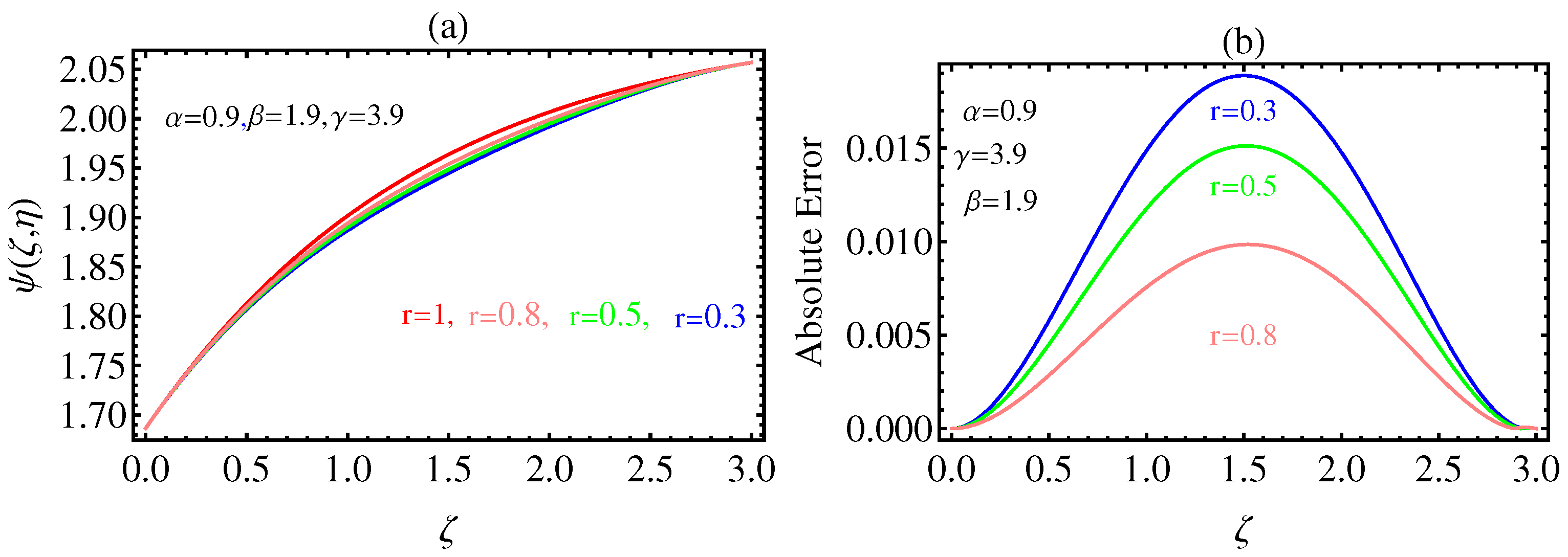
4. Numerical Results and Graphical Illustrations

In this section, we present the numerical results of the multi-space fractal-fractional Kuramoto-Sivashinsky equation and the multi-space fractal-fractional Korteweg-de Vries equation based on the generalized Mittag-Leffler kernel.

We first study the numerical results for the multi-space fractal-fractional Kuramoto-Sivashinsky equation. We focus on investigating two cases; the first case via the different values of the fractional order and the second case via different values of the fractional parameters. Figure 1a shows the comparison between the numerical solutions and the exact solutions of (17) for different values of fractional order with the fractal order fixed. In this figure, we set the fractional order as $\alpha =0.7,$ $\beta =1.7,$ $\vartheta =3.7$ and $\alpha =0.8,$ $\beta =1.8,$ $\vartheta =3.8$ and $\alpha =0.9,$ $\beta =1.9,$ $\vartheta =3.9$. This is illustrated by pink line, green line and blue line, respectively. For the exact solution, we illustrate by red line the case when $c=1,$ ${\xi }_0=-10,$ $\omega =\frac{1}{2}\sqrt{\frac{11}{9}},$ $m=5$ and $\tau ={10}^{-3}.$ In addition, in Figure 1b, the absolute error between the exact solution and the numerical solution for different values of the fractional order is represented for the same parameters as in Figure 1a. It can be seen from these two figures that the numerical solution approaches the exact solution as r approaches 1. This is evident in Figure 1b, where the value of the absolute error decreases as r approaches 1.

Figure 2a displays the comparison between the numerical solutions and the exact solutions of (17). In this case, we consider the values of $\alpha ,$$\beta$ and $\gamma$ as $0.9,$ $1.9$ and $3.9,$ respectively, for different values of r and with $c=1,$ ${\xi }_0=-11,$ $\omega =\frac{1}{2}\sqrt{\frac{11}{9}},$ $m=5$ and $\tau ={10}^{-3}.$ Figure 2b represents the absolute error between the numerical solutions and the exact solutions of (17) for the same data as in Figure 2a. The results for these figures show the qualitative behavior for the numerical solutions and the absolute errors in both cases. The error decreases significantly as the fractal and fractional orders approach the classical case.

In Figure 3, the residual error function in the fractal-fractional case for different values of r is represented. In this figure, the values are $r=0.4, 0.6$ and $0.9$ with $\alpha =0.9,$ $\beta =1.9,$ $\gamma =3.9,$ $c=1,$ ${\xi }_0=-10,$ $\omega =\frac{1}{2}\sqrt{\frac{11}{9}},$ $m=5$ and $\tau ={10}^{-3}.$ Also, from this figure, we derive the same conclusion as in Figure 1 and Figure 2, but here with the fractal-fractional order.

In a similar manner as we described above, we study the numerical results of the multi-space fractal-fractional Korteweg-de Vries equation. Figure 4a shows a comparison between the exact solution and the numerical solutions of the multi-space fractal-fractional Korteweg-de Vries equation for different values of r with $\alpha =0.7,$ $\beta =2.7,$ $\sigma =0.5,$ $m=4$ and $\tau ={10}^{-3}.$ while Figure 4b shows the absolute error between the exact solution and the numerical solutions for the same parameters as in Figure 4a.

Figure 5 displays the residual error function in the fractal-fractional case for different values of r for the multi-space fractal-fractional Korteweg-de Vries equation. Just as in the previous cases, there is a good agreement between the numerical results for the exact solution as well as an approximate solution. Although the numerical solutions are taken in the fractal and fractional cases, there is a good agreement. The clarification increases when the residual error function is represented in Figure 5.

5. Conclusions

In this paper, we have studied the multi-space fractal-fractional Kuramoto-Sivashinsky equation and the multi space fractal-fractional Korteweg-de Vries equation in the presence of a generalized Mittag-Leffler kernel. We have first introduced the fractal-fractional derivative by means of a generalized Mitag-Leffler kernel. We have then investigated its application on power functions. The case that we have studied here is a generalization of several previously-studied cases. The numerical results have been obtained by using the spectral collocation method with the aid of the shifted Legendre polynomials. With a view to verifying the numerical results, the absolute error between the exact and numerical solutions of the multi-space fractal-fractional Kuramoto-Sivashinsky equation and the multi space fractal-fractional Korteweg-de Vries equation have been calculated and we have thereby found a good agreement. In addition, the residual error function has been calculated for both of the above-mentioned equations. The error order has been shown to be small and it decreases as we go to the classical case for each of these equations. All of the numerical solutions have been obtained by using the computer program package Mathematica.

References

1. Kilbas, A.A.; Srivastava, H.M.; Trujillo, J.J. Theory and Applications of Fractional Differential Equations. In North-Holland Mathematical Studies; Elsevier (North-Holland) Science Publishers: Amsterdam, The Netherlands; London, UK; New York, NY, USA, 2006; Volume 204. [Google Scholar]
2. Podlubny, I. Fractional Differential Equations, to Methods of Their Solution and Some of Their Applications. In Mathematics in Science and Engineering; Academic Press: New York, NY, USA; London, UK; Sydney, Australia; Tokyo, Japan; Toronto, ON, Canada, 1999; Volume 198. [Google Scholar]
3. Srivastava, H.M. An introductory overview of fractional-calculus operators based upon the Fox-Wright and related higher transcendental functions. J. Adv. Eng. Comput. 2021, 5, 135–166. [Google Scholar] [CrossRef]
4. Alderremy, A.A.; Gómez-Aguilar, J.F.; Aly, S.; Saad, K.M. A fuzzy fractional model of coronavirus (COVID-19) and its study with Legendre spectral method. Results Phys. 2021, 21, 103773. [Google Scholar] [CrossRef] [PubMed]
5. Izadi, M.; Srivastava, H.M. A novel matrix technique for multi-order pantograph differential equations of fractional order. Proc. R. Soc. A Math. Phys. Eng. Sci. 2021, 477, 2021031. [Google Scholar] [CrossRef]
6. Saad, K.M.; Alqhtani, M. Numerical simulation of the fractal-fractional reaction diffusion equations with general nonlinear. AIMS Math. 2021, 6, 3788–3804. [Google Scholar] [CrossRef]
7. Kumar, S.; Pandey, R.K.; Srivastava, H.M.; Singh, G.N. A convergent collocation approach for generalized fractional integro-differential equations using Jacobi poly-fractonomials. Mathematics 2021, 9, 979. [Google Scholar] [CrossRef]
8. He, J.-H. Variational iteration method: A kind of nonlinear analytical technique: Some examples. Int. J. Non-Linear Mech. 1999, 34, 708–799. [Google Scholar] [CrossRef]
9. Saad, K.M.; Al-Sharif, E.H.F. Analytical study for time and time-space fractional Burgers equation. Adv. Differ. Equ. 2017, 2017, 300. [Google Scholar] [CrossRef] [Green Version]
10. Shi, X.-C.; Huang, L.-L.; Zeng, Y. Fast Adomian decomposition method for the Cauchy problem of the time-fractional reaction diffusion equation. Adv. Mech. Eng. 2016, 8, 1687814016629898. [Google Scholar] [CrossRef]
11. Bueno-Orovio, A.; Kay, D.; Burrage, K. Fourier spectral methods for fractional-in-space reaction-diffusion equations. BIT Numer. Math. 2014, 54, 937954. [Google Scholar] [CrossRef]
12. Takeuchi, Y.; Yoshimoto, Y.; Suda, R. Second order accuracy finite difference methods for space-fractional partial differential equations. J. Comput. Appl. Math. 2017, 320, 101–119. [Google Scholar] [CrossRef]
13. Cenesiz, Y.C.; Keskin, Y.; Kurnaz, A. The solution of the Bagley-Torvik equation with the generalized Taylor collocation method. J. Frankl. Inst. 2010, 347, 452–466. [Google Scholar] [CrossRef]
14. Srivastava, H.M.; Aomari, A.-K.N.; Saad, K.M.; Hamanah, W.M. Some dynamical models involving fractional-order derivatives with the Mittag-Leffler type kernels and their applications based upon the Legendre spectral collocation method. Fractal Fract. 2021, 5, 131. [Google Scholar] [CrossRef]
15. Saad, K.M. New fractional derivative with non-singular kernel for deriving Legendre spectral collocation method. Alex. Eng. J. 2020, 59, 1909–1917. [Google Scholar] [CrossRef]
16. Abdeljawad, T. A Lyapunov type inequality for fractional operators with nonsingular Mittag-Leffler kernel. J. Inequalities Appl. 2017, 2017, 130. [Google Scholar] [CrossRef]
17. Atangana, A. Fractal-fractional diferentiation and integration: Connecting fractal calculus and fractional calculus to predict complex system. Chaos Solitons Fractals 2017, 102, 396–406. [Google Scholar] [CrossRef]
18. Atangana, A.; Qureshi, S. Modeling attractors of chaotic dynamical systems with fractal-fractional operators. Chaos Solitons Fractals 2019, 123, 320–337. [Google Scholar] [CrossRef]
19. Saad, K.M.; Khader, M.M.; Gómez-Aguilar, J.F.; Baleanu, D. Numerical solutions of the fractional Fisher’s type equations with Atangana-Baleanu fractional derivative by using spectral collocation methods. Chaos Interdiscip. J. Nonlinear Sci. 2019, 29, 023116. [Google Scholar] [CrossRef]
20. Hosseininia, M.; Heydari, M.H.; Avazzadeh, Z. The numerical treatment of nonlinear fractal-fractional 2D Emden-Fowler equation utilizing 2D Chebyshkov polynomials. Fractals 2020, 28, 2040042. [Google Scholar] [CrossRef]
21. Khalil, H.; Khan, R.A.; Al-Smadi, M.H.; Freihat, A.A.; Shawagfeh, N. New operational matrix for shifted Legendre polynomials and fractional differential equations with variable coefficients. Punjab Univ. J. Math. 2015, 47, 1–23. [Google Scholar]
22. Srivastava, H.M.; Saad, K.M. A comparative study of the fractional-order clock chemical model. Mathematics 2020, 8, 1436. [Google Scholar] [CrossRef]
23. Lebedev, N.N. Special Functions and Their Applications; Silverman, R.A., Translator; Dover Publications: New York, NY, USA, 1972. [Google Scholar]
24. Khader, M.M. On the numerical solution and convergence study for system of non-linear fractional diffusion equations. Can. J. Phys. 2014, 92, 1658–1666. [Google Scholar] [CrossRef]
25. Khater, A.H.; Temsah, R.S. Numerical solutions of the generalized Kuramoto-Sivashinsky equation by Chebyshev spectral collocation methods. Comput. Math. Appl. 2008, 56, 1465–1472. [Google Scholar] [CrossRef] [Green Version]
26. Kuramoto, Y. Diffusion-induced chaos in reaction systems. Prog. Theor. Phys. Suppl. 1978, 64, 346–367. [Google Scholar] [CrossRef]
27. Sivashinsky, G.I. Nonlinear analysis of hydrodynamic instability in laminar flames. I. Derivation of basic equations. Acta Astronaut. 1977, 4, 1177–1206. [Google Scholar] [CrossRef]
28. Sivashinsky, G.I. On flame propagation under conditions of stoichiometry. SIAM J. Appl. Math. 1980, 39, 67–82. [Google Scholar] [CrossRef]
29. Liu, X. Gevrey class regularity and approximate inertial manifolds for the Kuramoto-Sivashinsky equation. Physica D Nonlinear Phenom. 1991, 50, 135–151. [Google Scholar] [CrossRef]
30. Grimshaw, R.; Hooper, A.P. The non-existence of a certain class of travelling wave solutions of the Kuramoto-Sivashinsky equation. Physica D Nonlinear Phenom. 1991, 50, 231–238. [Google Scholar] [CrossRef]
31. Baldwin, D.; Goktas, U.; Hereman, W.; Hong, L.; Martino, R.S.; Miller, J.C. Symbolic computation of exact solutions expressible in hyperbolic and elliptic functions for nonlinear PDEs. J. Symb. Comput. 2004, 37, 669–705. [Google Scholar] [CrossRef] [Green Version]
32. Parkes, E.J.; Duffy, B.R. An automated tanh-function method for finding solitary wave solutions to non-linear evolution equations. Comput. Phys. Commun. 1996, 98, 288–300. [Google Scholar] [CrossRef]
33. Korteweg, D.J.; de Vries, G. On the change of form of long waves advancing in a rectangular canal and on a new type of long stationary waves. Philos. Mag. 1895, 539, 422–443. [Google Scholar] [CrossRef]
34. Yang, X.-J.; Hristov, J.; Srivastava, H.M.; Ahmad, B. Modelling fractal waves on shallow water surfaces via local fractional Korteweg-de Vries equation. Abstr. Appl. Anal. 2014, 2014, 278672. [Google Scholar] [CrossRef] [Green Version]
35. Fung, M.-K. KdV equation as an Euler-Poincaré equation. Chin. J. Phys. 1997, 35, 789–796. [Google Scholar]
36. Zabusky, N.J.; Kruskal, M.D. Interaction of “Solitons” in a collisionless plasma and the recurrence of initial states. Phys. Rev. Lett. 1965, 15, 240–243. [Google Scholar] [CrossRef] [Green Version]
Figure 1. (a) Comparison Between the Exact Solution and the Numerical Solutions of (17) for Different Values of α , β and γ with r = 1 , c = 1 , ξ 0 = 11 , ω = 1 2 11 9 , m = 5 and τ = 10 3 . (b) Absolute Error Between the Exact Solution and the Numerical Solutions for the Same Parameters as in (a). (Red Line: Exact Solution).
Mathematics 10 01089 g001
Figure 2. (a) Comparison Between the Exact Solution and the Numerical Solutions of the Multi-Space Fractal-Fractional Kuramoto-Sivashinsky Equation for Different Values of r with α = 0.9 , β = 1.9 , γ = 3.9 , c = 1 , ξ 0 = 10 , ω = 1 2 11 9 , m = 5 and τ = 10 3 . (b) Absolute Error Between the Exact Solution and the Numerical Solutions for the Same Parameters as in (a). (Red Line: Exact Solution).
Mathematics 10 01089 g002
Figure 3. Residual Error Function of the Multi-Space Fractal-Fractional Kuramoto-Sivashinsky Equation for r = 0.4 ,   0.6 and 0.9 with α = 0.9 , β = 1.9 , γ = 3.9 , c = 1 , ξ 0 = 10 , ω = 1 2 11 9 , m = 5 and τ = 10 3 .
Mathematics 10 01089 g003
Figure 4. (a) Comparison Between the Exact Solution and the Numerical Solutions of the Multi-Space Fractal-Fractional Korteweg-de Vries Equation for Different Values of r with α = 0.7 , β = 2.7 , σ = 0.5 , m = 4 and τ = 10 3 . (b) Absolute Error Between the Exact Solution and the Numerical Solutions for the Same Parameters as in (a). (Red line: Exact solution).
Mathematics 10 01089 g004
Figure 5. Residual Error Function of the Multi-Space Fractal-Fractional Korteweg-de Vries Equation for r = 0.7 ,   0.8 ,   0.9 with α = 0.7 , β = 2.7 , σ = 0.5 , m = 4 and τ = 10 2 .
Mathematics 10 01089 g005
Publisher’s Note: MDPI stays neutral with regard to jurisdictional claims in published maps and institutional affiliations.