Probabilistic Linguistic Matrix Game Based on Fuzzy Envelope and Prospect Theory with Its Application

Abstract

Game theory is a powerful tool in modeling strategic interaction among rational players. However, as practical problems become more complex, uncertainty inevitably appears in the game. Due to the advantages of probabilistic linguistic term sets (PLTSs) in comprehensively and flexibly portraying uncertainty, fuzziness and hesitancy, this paper uses PLTSs to express players’ payoff values, and aims to develop an integrated method based on fuzzy envelope and prospect theory (PT) under a probabilistic linguistic environment for solving matrix games. In this method, an improved probabilistic ordered weighted averaging (POWA) operator is defined. Then, a novel trapezoidal fuzzy envelope for PLTSs is proposed and some related theorems are analyzed. Next, based on the defined cosine distance measure for PLTSs, the players’ psychological behavior in the game is considered by establishing the prospect value function. Besides, the applicability and practicability of the proposed method is verified with an example from the development strategy of Sanjiangyuan National Nature Reserve (SNNR) in China. Finally, some comparative analyses are carried out to illustrate the superiority of the proposed method. In order to improve the application of this proposed method, a decision support system (DSS) based on it is designed.

1. Introduction

Nowadays, human society is faced with a variety of decision-making problems, which are usually characterized by complexity, diversity and uncertainty. Fortunately, game theory has a powerful ability to handle such complex decision-making problems. Compared with other theories, game theory is prominent in revealing the inherent laws of socio-economic phenomena and the essential characteristics of human behavior. Game theory is a useful tool in studying the interaction between groups, individuals or players [1]. It has been widely applied in many fields, such as politics [2], economics [3], military [4] and environmental decision-making [1]. As we all know, to create a game model, some assumptions are required about the type of game, the strategies of players and the payoff values. With the increase in the number of players and strategies, the number of payoff values given by players in a game will increase significantly, which will undoubtedly bring a heavy burden to them [5]. Moreover, due to the increasing complexity of the game environment and the inevitable uncertainty that arises in the game, finding a suitable method to describe inaccuracy is urgent [6]. This research focuses on a matrix game with uncertain information.

Generally, there are three commonly-used representations that can depict the inaccuracy of the payoff values in a matrix game model: intervals [7], fuzzy information [8,9,10,11,12,13,14,15,16] and linguistic information [5,6,17,18,19]. Considering the ambiguity of human thinking and the lack of available information, players may prefer to express their opinions with linguistic information rather than interval numbers or fuzzy numbers [20]. For example, teachers prefer to use linguistic terms (e.g., “medium”, “good” and “excellent”) to evaluate children’s performance in kindergarten. In fact, a single linguistic term is insufficient to perfectly express the decision-makers’ (DMs’) evaluation. To handle this shortcoming, Rodríguez et al. [21] put forward the concept of the hesitant fuzzy linguistic term set (HFLTS), which can improve the richness and flexibility of linguistic information acquisition. However, HFLTS does not reflect the probability of linguistic terms, which may result in the loss of original information. To overcome this issue, Pang et al. [22] proposed the concept of the probabilistic linguistic term set (PLTS).A PLTS permits players to select multiple linguistic terms from a linguistic term set (LTS) and assign them with probabilities, which can describe players’ judgments more exactly [23]. A PLTS combines fuzziness, hesitancy and accurate information in a comprehensive form. Therefore, it is appropriate to use PLTSs to represent the payoff values of a matrix game. PLTS has been widely used by investigators [24,25,26,27,28] since it was proposed. However, to the best of our knowledge, probabilistic linguistic information is rarely used to depict the payoff values of matrix games. This is the first of the research gaps intended to be narrowed.

There are many defuzzification techniques which deal with uncertain information in matrix games, such as membership function [5], membership function and non-membership function [12], similarity degree [13], value function and fuzzy function [14], ranking function [15], cut sets [16], etc. For matrix games with linguistic information, the semantics of linguistic terms may be lost by substituting symbolic computation for the operation of membership functions during computation [5]. The use of membership function is very important in the defuzzification of probabilistic linguistic information [6], but these methods [18,29] integrate the linguistic terms in the game without introducing the membership function. However, as far as we know, there is no research on the trapezoidal membership function of probabilistic linguistic information. This is the second research gap intended to be covered.

Prospect theory (PT) [30] was used to portray the psychological behavior of DMs under risk. Although the PT has been extended into various fuzzy environments [31,32,33,34] to solve multi-attribute decision making (MADM) problems, the PT was first studied in [6] to solve a matrix game under a hesitant fuzzy linguistic environment. However, to the best of our knowledge, there is no research on introducing PT under a probabilistic linguistic environment to solve a matrix game problem. This is the third research gap that needs to be filled.

There are three challenges to overcome in the process of filling the above research gaps: (i) how to build a matrix game model under a probabilistic linguistic environment is the first challenge; (ii) how to defuzzify the probabilistic linguistic information with trapezoidal membership function is the second challenge; (iii) how to introduce the PT to solve a matrix game under probabilistic linguistic environment is the third challenge.

Motivated by the aforesaid analysis, this study aims to propose a probabilistic linguistic matrix game (PLMG) method based on fuzzy envelope and PT, and the effectiveness and practicality of the proposed method is verified by an example from the development strategy of Sanjiangyuan National Nature Reserve (SNNR).It is essential to propose such a method due to the following reasons. Firstly, the study of matrix games under a probabilistic linguistic environment expands the scope of application of game theory. Secondly, the definition of trapezoidal fuzzy envelop for probabilistic linguistic information enriches the defuzzification technology for linguistic information. Moreover, the fusion of PT commendably captures the DMs’ psychological behavior regarding gain and loss, which makes the proposed method more suitable for solving practical decision-making problems. In addition, the proposed method provides feasibility for solving MADM problems without weight information from the perspective of the game between DM and Nature. Finally, the proposed method not only fills the aforementioned research gaps, but has important practical value.

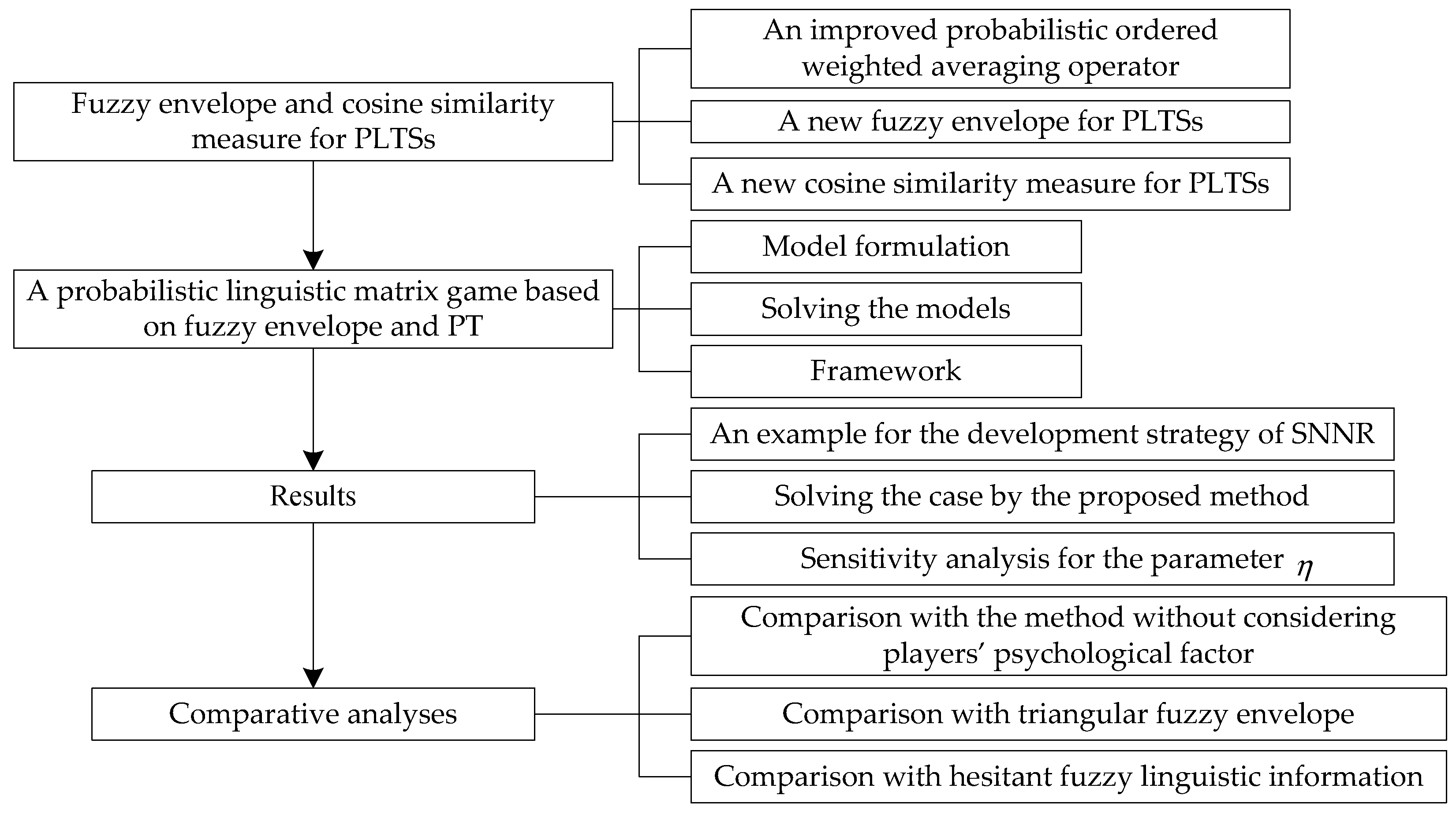
The rest of the paper is organized as follows: Section 2 briefly recalls the literature review of fuzzy matrix games, PLTSs and prospect theory (PT), and extracts the research gaps dealt with in this paper. Section 3 provides the essential preliminaries on trapezoidal fuzzy number (TrFN), HFLTS, PLTS, ordered weighted averaging (OWA) operators and PT; a research flow is also provided in this section. Section 4 gives the definitions of improved probabilistic ordered weighted averaging (POWA) operator, fuzzy envelope and cosine similarity measure for PLTSs, and then their related theorems are analyzed. Section 5 develops a probabilistic linguistic matrix game method based on fuzzy envelope and PT. Section 6 deals with an example fromthe development strategy of SNNR. Section 7 ends this paper with concluding remarks and prospects for the future research.

2. Literature Review and Research Gaps

This section recalls the reported progress on fuzzy matrix games, PLTSs and prospect theory. Afterwards, the research gaps dealt with in this paper are sketched.

2.1. Fuzzy Matrix Games

Up to now, fuzzy matrix games have been widely considered by scholars. Li [7,8,9] extended the matrix game into intervals, triangular fuzzy numbers and trapezoidal fuzzy numbers, separately. Yang et al. [10] developed a parametric linear programming method to deal with an intuitionistic fuzzy matrix game. Li [11] extended the matrix game method into an interval-valued intuitionistic fuzzy environment, and proved that each interval-valued intuitionistic fuzzy matrix game has a solution, which can be obtained through solving a pair of auxiliary linear/nonlinear programming models. Based on the definition of novel similarity measure, Jana and Roy [12] proposed four algorithms to seek the optimal value of the dual hesitant fuzzy matrix game with one restriction. Karmakar et al. [13] developed a matrix game under a type-2 intuitionistic fuzzy environment based on a new distance measure. Xue et al. [14] proposed the Ambika method of hesitant fuzzy matrix games to find the optimal solutions of mixed strategies by solving the converted linear programming models. As for matrix games with linguistic information, Singh et al. [18] put forward a two-tuple linguistic matrix game method to solve a MADM problem, which can generate the optimal weights for the attributes in an intermediate step. Verma and Aggarwal [19] developed a two-tuple intuitionistic fuzzy linguistic matrix game and gave the solution method. Xue et al. [6] studied the hesitant fuzzy linguistic matrix game method and solved it by constructing a two-objective programming model, which filled the theoretical gap in the game theory under a hesitant fuzzy linguistic environment. Although the above achievements have extended matrix games into various fuzzy and linguistic environments, there are few studies on extending matrix games into a probabilistic linguistic environment. Thus, the first research gap emerges.

2.2. PLTSs

PLTS was originally defined by Pang et al. [22] in 2016, and can provide players with multiple possible linguistic terms and corresponding probability information. So far, the research on PLTS has achieved fruitful results. As for the applications of PLTSs, Lin et al. [23] proposed a new score function for PLTSs (named as ScoreC-PLTS), based on which, the VIKOR and TOPSIS methods were respectively developed. You and Hou [24] put forward a novel feedback mechanism for probabilistic linguistic preference relations to solve a group decision-making problem. Xian et al. [25] developed an improved approach to comparing PLTSs and proposed a new decision-making method for solving the selection of a public opinion monitoring system. In addition, PLTSs have also been extended into numerous classical MADM methods to solve practical decision-making problems, such as TODIM [26], MULTIMOORA [27], ELECTRE [28], etc. In the applications of PLTS, the biggest challenge is how to address probabilistic linguistic information while minimizing the loss of original information. To overcome this challenge, the defuzzification techniques of PLTSs play a crucial role. Methods in [14,24,25,26,27] adopted the approach of ranking function by defining the score function, distance measure or similarity measure. Mi et al. [6] studied the defuzzification technology of PLTS by using a triangular fuzzy membership function. Based on the above analysis, it can be found that there is no research on the trapezoidal fuzzy membership function of probabilistic linguistic information. Therefore, the second research gap appears.

2.3. Prospect Theory

In many practical decision-making problems, the DMs’ psychological behavior regarding loss and gain is often ignored. Prospect theory (PT) [30] is an appropriate tool to portray the DMs’ psychological behavior under risk. The PT has been widely used by investigators since it was put forward. Metzger and Rieger [35] studied a framework for non-cooperative games in normal form where players have behavioral preferences following PT. To study the issue of watershed ecological compensation in Taihu Lake Basin, Shen et al. [36] established an evolutionary game model between local government and polluting enterprises based on PT. However, the above-mentioned research was conducted in a precise environment. In order to enrich the application of PT, it has been extended into various fuzzy environments, such as intuitionistic fuzzy environment [31], hesitant fuzzy environment [32], hesitant fuzzy linguistic environment [6,33], probabilistic linguistic environment [34], etc. Based on the above review, it can be found that there is no research on introducing PT under a probabilistic linguistic environment to solve matrix game problems. Thus, the third research gap arises.

2.4. Research Gaps

Although the abovementioned achievements are powerful in dealing with real decision problems, some research gaps still exist as follows:

• PLTS permits players to select multiple linguistic terms from a linguistic term set (LTS) and assign them with probabilities, which can describe players’ judgments more exactly [23]. A PLTS combines fuzziness, hesitancy and accurate information in a comprehensive form. Although PLTSs have been widely used by investigators [24,25,26,27,28] since they were proposed, probabilistic linguistic information is rarely used to depict the payoffs in matrix games. This is the first research gap intended to be narrowed.
• There are many defuzzification techniques [5,12,13,14,15,16,18,29] to address uncertain information. For matrix games with linguistic information, the semantics of linguistic terms may be lost by substituting symbolic computation for the operation of membership functions during computation [5]. The use of membership function is very important in the defuzzification of probabilistic linguistic information [6], but these methods [18,29] integrated the linguistic terms in the game without introducing the membership function. However, to the best of our knowledge, there is no research on the trapezoidal membership function of probabilistic linguistic information. This is the second research gap intended to be filled.
• Although PT has been extended into many fuzzy environments [6,31,32,33,34], most of them [31,32,33,34] are applied to solve MADM problems. The PT applied to solve a matrix game problem was first studied in [6]. However, as far as we know, there is no research on introducing PT under a probabilistic linguistic environment to solve a matrix game problem. This is the third research gap intended to be filled.

3. Methodology

This section recalls the basic concepts related to TrFNs, HFLTSs, PLTSs and the ordered weighted averaging (OWA) operator. Then, the prospect theory is also outlined.

3.1. Preliminaries

3.1.1. Related Concepts for TrFNs, HFLTSs and PLTSs

Definition 1

([37]). A TrFN can be represented by a four-tuple $\tilde{e}=(e_1,e_2,e_3,e_4)$, where $e_i$ $(i=1,2,3,4)$ are real numbers and meet $e_1\le e_2\le e_3\le e_4$. According to cut set theory, a TrFN $\tilde{e}=(e_1,e_2,e_3,e_4)$ is equivalent to the following interval:

$$\tilde{e}(\alpha )=[e^{-}(\alpha ),e^{+}(\alpha )]=[e_1+(e_2-e_1)\alpha ,e_4-(e_4-e_3)\alpha ]\alpha \in [0,1]$$

(1)

It can be observed that if $e_1=e_2=e_3=e_4=e$, then TrFN $\tilde{e}$ reduces to a crisp number $e$; If $e_2=e_3$, then TrFN $\tilde{e}$ generates to a triangular fuzzy number (TFN) $\tilde{e}=(e_1,e_2,e_4)$. Hence, TrFNs have the ability to generalize TFNs and crisp numbers.

Definition 2

([21]). Let $S=\{s_0,s_1,\cdots ,s_{\tau }\}$ be a linguistic term set. A HFLTS (denoted by $H_S$) is an ordered subset of the consecutive linguistic terms in $S$.

The following example is used to further understand the meaning of HFLTSs as defined above.

Example 1.

Let S = {s₀: extremely bad, s₁: very bad, s₂: bad, s₃: medium, s₄: good, s₅: very good, s₆: extremely good} be a linguistic term set. Then, $H_S^1=\left\{s_2\right\}$, $H_S^2=\{s_0,s_1,s_2\}$, $H_S^3=\{s_3,s_4,s_5\}$ and $H_S^4=\{s_4,s_5,s_6\}$ are four HFLTSs.

Although Rodríguez et al. [21] proposed a context-free grammar $G_H=(V_N,V_T,I,P)$ to produce comparative linguistic expressions, $G_H$ is not available in the computational process. Thus, a transformation function is defined as $T_{G_H}:S_{ll}\to H_S$ to transform linguistic expressions into HFLTSs, where $S_{ll}$ is the term domain yielded by $G_H$. Hence, four types of HFLTSs can be defined as follows:

• $T_{G_H}(s_i)=\left\{s_i\right|s_i\in S\}$;
• $T_{G_H}(\mathrm{at}\mathrm{most}{s}_i)=\left\{s_j\right|s_j\in S\mathrm{and}{s}_j\le s_i\}=\{s_0,s_1,\cdots ,s_{i-1},s_i\}$;
• $T_{G_H}(\mathrm{at}\mathrm{least}{s}_i)=\left\{s_j\right|s_j\in S\mathrm{and}{s}_j\ge s_i\}=\{s_i,s_{i+1},\cdots ,s_{\tau }\}$;
• $T_{G_H}(\mathrm{between}{s}_i\mathrm{and}{s}_j)=\left\{s_k\right|s_k\in S\mathrm{and}{s}_i\le s_k\le s_j\}=\{s_i,s_{i+1},\cdots ,s_{j-1},s_j\}$.

Definition 3

([22]). Let $S=\{s_0,s_1,\cdots ,s_{\tau }\}$ be a linguistic term set. A PLTS is defined as

$$P{L}_S=\{s_k(p_k)|s_k\in S,k=1,2,\cdots ,\#P{L}_S,0\le p_k\le 1,{\displaystyle {\sum }_{k=1}^{\#P{L}_S}{p}_k\le 1}\}$$

(2)

where $s_k(p_k)$ denotes the linguistic term $s_k$ assigned with a probability $p_k$, $\#P{L}_S$ is the number of linguistic terms in $P{L}_S$.

In order to facilitate subsequent calculations, this paper assumes that the linguistic terms in PLTSs are consecutive and have corresponding probabilities. Therefore, based on Definition 3 and four types of HFLTSs defined in [21], the four types of PLTSs also can be defined as follows.

Definition 4.

PLTSs can be divided into the following four types according to the implications of linguistic expressions

• $P{T}_{G_H}(s_i)=\{s_i(p_i)|s_i\in S,0\le p_i\le 1\}$;
• $\begin{array}{ll}P{T}_{G_H}(\mathrm{at}\mathrm{most}{s}_i)& =\{s_j(p_j)|s_j\in S,s_j\le s_i,0\le p_j\le 1,{\displaystyle {\sum }_{j=0}^i{p}_j\le 1}\}\\ & =\{s_0(p_0),\cdots ,s_{i-1}(p_{i-1}),s_i(p_i)\}\end{array}$;
• $\begin{array}{ll}P{T}_{G_H}(\mathrm{at}\mathrm{least}{s}_i)& =\{s_j(p_j)|s_j\in S,s_j\ge s_i,0\le p_j\le 1,{\displaystyle {\sum }_{j=i}^{\tau }{p}_j\le 1}\}\\ & =\{s_i(p_i),s_{i+1}(p_{i+1}),\cdots ,s_{\tau }(p_{\tau })\}\end{array}$;
• $\begin{array}{ll}P{T}_{G_H}(\mathrm{between}{s}_i\mathrm{and}{s}_j)& =\{s_k(p_k)|s_k\in S,s_i\le s_k\le s_j,0\le p_k\le 1,{\displaystyle {\sum }_{k=i}^j{p}_k\le 1}\}\\ & =\{s_i(p_i),\cdots ,s_j(p_j)\}\end{array}$.

3.1.2. Ordered Weighted Averaging Operator

Definition 5

([38]). Let $U=\{u_1,u_2,\cdots ,u_n\}$ be a set of arguments and $a_k$ be the k-th largest argument among set $U$. An ordered weighted averaging (OWA) operator can be defined as

$$OW{A}_W(u_1,u_2,\cdots ,u_n)={\displaystyle {\sum }_{k=1}^n{w}_k}{a}_k$$

(3)

where $w_k$ is the weight of $a_k$, meeting $0\le w_k\le 1$ and ${\displaystyle {\sum }_{k=1}^n{w}_k}=1$.

Definition 6

([39]). Let $\lambda \in [0,1]$ be a parameter. The first and second kinds of OWA weight vectors $W^o={(w_1^o,w_2^o,\cdots ,w_n^o)}^T$ and $W^p={(w_1^p,w_2^p,\cdots ,w_n^p)}^T$ are respectively defined as $w_1^o=\lambda ,w_2^o=\lambda (1-\lambda ),\cdots ,w_k^o=\lambda {(1-\lambda )}^{k-1},\cdots ,w_n^o={(1-\lambda )}^{n-1}$ and $w_1^p={\lambda }^{n-1},w_2^p=(1-\lambda ){\lambda }^{n-2},\cdots ,w_k^p=(1-\lambda ){\lambda }^{n-k},\cdots ,w_n^p=1-\lambda$.

Especially, when $n>2$, the orness degrees of $W^o$ and $W^p$ are respectively higher and lower than the value of the parameter $\lambda$. Filev and Yager [39] termed the $W^o$ and $W^p$ as optimistic and pessimistic exponential OWA operators, respectively.

3.1.3. Prospect Theory

In order to make up the shortage that DMs are entirely rational in the traditional “expected utility theory”, Kahneman and Tversky [30] first put forward PT to portray the psychological behavior of DMs under risk. PT is a descriptive model based on the hypothesis of bounded rationality, which validly reveals the practical decision-making behavior of individuals under risk and uncertainty.

PT is normally divided into editing and assessing stages. In the editing phase, DMs judge gains and losses by comparing the evaluation value with the reference point. A change in the reference point will result in a change in the DM’s perception of gains or losses. In the assessing phase, the gains and losses are converted into prospect values by the prospect value function. The prospect value function in the form of a power law is given as follows:

$$v(x)=\{\begin{array}{ll}{x}^{\varphi },& \mathrm{if}x\ge 0\\ -\epsilon {(-x)}^{\phi },& \mathrm{if}x<0\end{array}$$

(4)

where $x$ can be seen as the deviation between the reference point and assessment value. $x\ge 0$ means that the assessment value is greater than the reference point, and DMs will perceive gains. Conversely, $x<0$ indicates that the assessment value is smaller than the reference point, and DMs will perceive losses. $v(x)$ stands for the prospect value. Exponent parameters $\varphi$ $(\varphi \in [0,1])$ and $\phi$ $(\phi \in [0,1])$ are the risk aversion coefficient and risk preference coefficient, respectively. $\epsilon$ $(\epsilon \ge 1)$ represents the individual’s risk aversion grade, the larger the value of $\epsilon$, the higher the individual’s aversion to risk. It has been verified that when $\varphi =\phi =0.88$ and $\epsilon =2.25$, the experimental results are consistent with the original data [40,41].

3.2. Research Flow

In order to give readers a general understanding of the proposed method, this paper provides a flowchart of the proposed method as shown in Figure 1.

4. Fuzzy Envelope and Cosine Similarity Measure for PLTSs

In this section, an improved POWA operator is defined. Then, based on the improved POWA operator, an approach is developed to generate a fuzzy envelope for PLTS by using trapezoidal fuzzy membership functions. Ultimately, a cosine similarity measure for PLTSs is put forward.

4.1. An Improved Probabilistic Ordered Weighted Averaging Operator

Based on Definition 5 and inspired by the POWA operator [42], an improved POWA operator is defined as follows:

Definition 7.

Let$U=\{u_1,u_2,\cdots ,u_n\}$be a set of arguments and$a_k$be the k-th largest argument among set$U$. An improved POWA operator can be defined as

$$POW{A}_{\widehat{W}}(u_1,u_2,\cdots ,u_n)={\displaystyle {\sum }_{k=1}^n{\widehat{w}}_k}{a}_k$$

(5)

where${\widehat{w}}_k=w_k{p}_k/{\displaystyle {\sum }_{k=1}^n{w}_k{p}_k}$,$w_k$($p_k$) is the weight (probability) associated with argument$a_k$.

In order to apply Equation (5) to aggregate the arguments, the values of $p_k$ and $w_k$ should be determined first. Generally, the former can be derived from DMs’ subjective judgments, and the latter can be calculated by using a series of approaches. Since the OWA operator weight-determining approach in [39] has the powerful ability to identify the pessimistic and optimistic OWA operator weights by orness measure, this paper intends to employ it to determine the OWA operator weights with probability information (called POWA weights hereafter).

For the convenience of the following calculation, denote ${\widehat{W}}^o={({\widehat{w}}_1^o,{\widehat{w}}_2^o,\cdots ,{\widehat{w}}_n^o)}^T$ with ${\widehat{w}}_k^o=w_k^o{p}_k/{\displaystyle {\sum }_{k=1}^n{w}_k^o{p}_k}$ and ${\widehat{W}}^p={({\widehat{w}}_1^p,{\widehat{w}}_2^p,\cdots ,{\widehat{w}}_n^p)}^T$ with ${\widehat{w}}_k^p=w_k^p{p}_k/{\displaystyle {\sum }_{k=1}^n{w}_k^p{p}_k}$ $(k=1,2,\cdots ,n)$, where the $w_k^o$ and $w_k^p$ are decided by Definition 6.

Remark 1.

Merigo and Wei [42] proposed a POWA operator by introducing ${\widehat{w}}_k=\beta w_k+(1-\beta )p_k$. When the probabilities of all arguments are equal, the POWA operator (see Equation (2) in [42]) should be reduced into the classical OWA operator (see Equation (3) in Definition 5), namely, for all $k=1,2,\cdots ,n$ it holds that ${\widehat{w}}_k=w_k$ if $p_k$ is a non-zero constant. However, it cannot be deduced ${\widehat{w}}_k=w_k$ from ${\widehat{w}}_k=\beta w_k+(1-\beta )p_k$, which indicates that Merigo and Wei’s [42] POWA operator failed to consider the case that the probabilities of all arguments are equal. Fortunately, the proposed improved POWA operator can tackle this issue perfectly, since ${\widehat{w}}_k=w_k{p}_k/{\displaystyle {\sum }_{k=1}^n{w}_k{p}_k}$ can reduce to ${\widehat{w}}_k=w_k$ when all $p_k$ $(k=1,2,\cdots ,n)$ equal a non-zero constant.

Remark 2.

In the traditional methods [24,25,26,27,28], the probability information is incomplete (i.e., ${\displaystyle {\sum }_{k=1}^n{p}_k}<1$), yet it is required to normalize the PLTSs for further calculation. However, in the proposed improved POWA operator, there is no need to normalize the PLTSs in this paper, which can preserve more of the initial information from the DMs.

4.2. A New Fuzzy Envelope for PLTSs

PLTSs have powerful capability to tackle linguistic decision-making problems flexibly. To facilitate the calculation process based on PLTSs, a new fuzzy envelop of PLTS employing trapezoidal fuzzy membership function is proposed. To achieve such a fuzzy representation, the following factors should be considered:

• The different probabilities of linguistic terms imply the different importance of such terms.
• Trapezoidal fuzzy membership function has strong ability to portray the fuzziness of the comparative linguistic terms.
• The parameters of the trapezoidal fuzzy membership function are calculated by an aggregation operator, which can embody the different importance of the linguistic terms in PLTS.

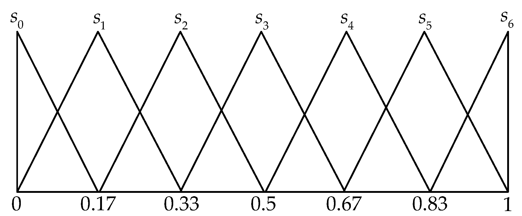
A LTS can be defined as $S=\left\{s_i\right|i=0,1,\cdots ,\tau \}$, where $s_i$ stands for a possible value for a linguistic variable and $\tau$ is an even and positive integer. Let S = {s₀: extremely bad, s₁: very bad, s₂: bad, s₃: medium, s₄: good, s₅: very good, s₆: extremely good} be a LTS (i.e., $\tau =6$). Afterwards, S with its semantics depicted by triangular fuzzy membership function can be visually displayed in Figure 2 [43].

Presume that all the linguistic terms $s_k\in S$ can be represented as a triangular fuzzy number $\tilde{A}=\{a_k^l,a_k^m,a_k^u\}$ ($k=0,1,\cdots ,\tau$). Particularly when $\tau =6$, the linguistic terms can be shown in Figure 2. Hence, PLTS $P{H}_S$ can be formed as $\tilde{A}=\{a_0^l,a_0^m,a_1^l,a_0^u,a_1^m,a_2^l,\cdots ,a_{\tau }^l,a_{\tau -1}^u,a_{\tau }^m,a_{\tau }^u\}$. The elements contained in $\tilde{A}$ can be further simplified as $\tilde{A}=\{a_0^l,a_0^m,a_1^m,a_2^m,\cdots ,a_{\tau }^m,a_{\tau }^u\}$ due to $a_{k-1}^u=a_k^m=a_{k+1}^l$. Then, a fuzzy envelope of PLTS based on the proposed improved POWA operator is defined as follows.

Definition 8.

For a PLTS$P{L}_S$, its fuzzy envelope$env(P{L}_S)$can be defined as a trapezoidal fuzzy membership function$Tr(b_1,b_2,b_3,b_4)$, i.e.,$env(P{L}_S)=Tr(b_1,b_2,b_3,b_4)$.

In order to obtain the fuzzy envelope $env(P{L}_S)$, it is required to determine the values of the parameters $b_1$, $b_2$, $b_3$ and $b_4$. Next, the following laws are presented to determine the values of the parameters $b_1$, $b_2$, $b_3$ and $b_4$ for different situations.

• Fuzzy envelope for $P{T}_{G_H}(s_i)$. The parameters $b_1$, $b_2$, $b_3$ and $b_4$ are determined as $(b_1,b_2,b_3,b_4)=(a_i^l,a_i^m,a_i^m,a_i^u)$;
• Fuzzy envelope for $P{T}_{G_H}(\mathrm{at}\mathrm{most}{s}_i)$. $T_{G_H}(\mathrm{at}\mathrm{most}{s}_i)$ can be transformed into $\tilde{A}=\{a_0^l,a_0^m,a_1^m,\cdots ,a_i^m,a_i^u\}$. The parameters $b_1$, $b_2$, $b_4$ and $b_3$ are determined as $b_1=b_2=\min \{a_0^l,a_0^m,a_1^m,\cdots ,a_i^m,a_i^u\}=a_0^l$, $b_4=\max \{a_0^l,a_0^m,a_1^m,\cdots ,a_i^m,a_i^u\}=a_i^u$ and

  $$b_3=POW{A}_{{\widehat{W}}^o}(a_0^m,a_1^m,\cdots ,a_i^m)$$

  (6)

Herein, $n=i+1$. Then, $w_1^o=\lambda ,w_2^o=\lambda (1-\lambda ),\cdots ,w_k^o=(1-\lambda ){\lambda }^{k-1},\cdots ,w_{i+1}^o={(1-\lambda )}^i$.

Theorem 1.

Parameter$b_3$determined by Equation (6) owns the following properties.

• $0=a_0^m\le b_3\le a_i^m\le 1$;
• For fixed$s_i$and$W^o$, if the probability of$a_i^m$is closer to 1, then$b_3$is closer to$a_i^m$; if the probability of$a_0^m$is closer to 1, then$b_3$is closer to$a_0^m$;
• Let$p_k=r$$(k=0,1,2,\cdots ,i)$, where$0<r<1$. For a fixed$s_i$, if$\lambda \to 0$, then$b_3\to a_0^m$; if$\lambda \to 1$, then$b_3\to a_i^m$.

Proof of Theorem 1.

• Since $\min \{a_0^m,a_1^m,\cdots ,a_i^m\}=a_0^m=0$, $\max \{a_0^m,a_1^m,\cdots ,a_i^m\}=a_i^m\le 1$ and $b_3$ is derived by the operator $POW{A}_{{\widehat{W}}^o}$, $b_3$ is between the minimum and maximum aggregated values (i.e., $a_0^m$ and $a_i^m$).
• For convenience, the probability of $a_i^m$ is denoted by $p_0$. For a fixed weight vector $W^o={(w_1^o,w_2^o,\cdots ,w_n^o)}^T$, the closer the value of $p_0$ is to 1, the larger the value of ${\widehat{w}}_0^o$, which will result in the value of ${\widehat{w}}_0^o{a}_i^m$ being closer to $a_i^m$. Hence, for fixed $s_i$ and $W^o$, if $p_0$ is closer to 1, then $b_3$ is closer to $a_i^m$. It can be deduced that the property “for fixed $s_i$ and $W^o$, if $p_{i+1}$ is closer to 1, then $b_3$ is closer to $a_0^m$” also holds.
• Since $p_k=r$ $(k=0,1,2,\cdots ,i)$, where $0<r<1$, it holds that ${\widehat{w}}_k^o=w_k^o$. In this case, if $\lambda \to 0$, then ${\widehat{w}}_1^o\to 0,{\widehat{w}}_2^o\to 0,\cdots ,{\widehat{w}}_i^o\to 0$ and ${\widehat{w}}_{i+1}^o\to 1$, which indicates that $b_3\to {\widehat{w}}_{i+1}^o{a}_0^m\to a_0^m$. The property “if $\lambda \to 1$, then $b_3\to a_i^m$” can be proven similarly.

This completes the proof of Theorem 1. □

• Fuzzy envelope for $P{T}_{G_H}(\mathrm{at}\mathrm{least}{s}_i)$. $T_{G_H}(\mathrm{at}\mathrm{least}{s}_i)$ can be transformed into $\tilde{A}=\{a_i^l,a_i^m,a_{i+1}^m,\cdots ,a_{\tau }^m,a_{\tau }^u\}$. The parameters $b_1$, $b_3$, $b_4$ and $b_2$ are determined as $b_1=\min \{a_i^l,a_i^m,a_{i+1}^m,\cdots ,a_{\tau }^m,a_{\tau }^u\}=a_i^l$, $b_3=b_4=\max \{a_i^l,a_i^m,a_{i+1}^m,\cdots ,a_{\tau }^m,a_{\tau }^u\}=a_{\tau }^u$,

  $$b_2=POW{A}_{{\widehat{W}}^p}(a_i^m,a_{i+1}^m,\cdots ,a_{\tau }^m)$$

  (7)

  Herein, $n=\tau -i+1$. Then, $w_1^p={\lambda }^{\tau -i}$, $w_2^p=(1-\lambda ){\lambda }^{\tau -i-1}$, $\cdots ,$ $w_k^p=(1-\lambda ){\lambda }^{\tau -i-k+1},\cdots ,$ $w_{\tau -i+1}^p=1-\lambda$.

Theorem 2.

Parameter$b_2$determined by Equation (7) owns the following properties:

• $0\le a_i^m\le b_2\le a_{\tau }^m=1$;
• For fixed$s_i$and$W^p$, if the probability of$a_{\tau }^m$is closer to 1, then $b_2$ is closer to $a_{\tau }^m$ ; if the probability of $a_i^m$ is closer to 1, then $b_2$ is closer to $a_i^m$;
• Let$p_k=r$$(k=0,1,2,\cdots ,\tau -i)$, where$0<r<1$. For a fixed$s_i$, if$\lambda \to 0$, then$b_2\to a_i^m$; if$\lambda \to 1$, then$b_2\to a_{\tau }^m$.

Proof of Theorem 2.

• Since $\min \{a_i^m,a_{i+1}^m,\cdots ,a_{\tau }^m\}=a_i^m\ge 0$, $\max \{a_i^m,a_{i+1}^m,\cdots ,a_{\tau }^m\}=a_{\tau }^m=1$ and $b_2$ is obtained by the $POW{A}_{{\widehat{W}}^p}$ operator, $b_2$ is between the minimum and maximum aggregated values.
• For convenience, the probability of $a_{\tau }^m$ is denoted by $p_0$. For a fixed weight vector $W^p={(w_1^p,w_2^p,\cdots ,w_n^p)}^T$, the closer the value of $p_0$ is to 1, the larger the value of ${\widehat{w}}_0^p$, which will cause the value of ${\widehat{w}}_0^p{a}_{\tau }^m$ to be closer to $a_{\tau }^m$. Hence, for fixed $s_i$ and $W^p$, if $p_0$ is closer to 1, then $b_2$ is closer to $a_{\tau }^m$. It also can be inferred that the property “for fixed $s_i$ and $W^p$, if $p_{\tau -i+1}$ is closer to 1, then $b_2$ is closer to $a_i^m$”.
• Since $p_k=r$ $(k=0,1,2,\cdots ,\tau -i)$, where $0<r<1$, it holds that ${\widehat{w}}_k^p=w_k^p$. In this case, if $\lambda \to 0$, then ${\widehat{w}}_1^p\to 0,{\widehat{w}}_2^p\to 0,\cdots ,{\widehat{w}}_{\tau -i}^p\to 0$ and ${\widehat{w}}_{\tau -i+1}^p\to 1$, which shows that $b_2\to {\widehat{w}}_{\tau -i+1}^p{a}_i^m\to a_i^m$. The property “if $\lambda \to 1$, then $b_2\to a_{\tau }^m$” can also be proven.

This completes the proof of Theorem 2. □

• Fuzzy envelope of $P{T}_{G_H}(\mathrm{between}{s}_i\mathrm{and}{s}_j)$. $T_{G_H}(\mathrm{between}{s}_i\mathrm{and}{s}_j)$ can be transformed into $\tilde{A}=\{a_i^l,a_i^m,a_{i+1}^m,\cdots ,a_j^m,a_j^u\}$. The parameters $b_1$ and $b_4$ are determined as $b_1=\min \{a_i^l,a_i^m,a_{i+1}^m,\cdots ,a_j^m,a_j^u\}=a_i^l$ and $b_4=\max \{a_i^l,a_i^m,a_{i+1}^m,\cdots ,a_j^m,a_j^u\}=a_j^u$; For determination for the parameters $b_2$ and $b_3$, it is required to consider the parity of $i+j$.

  (i)

  If $i+j$ is odd, then

  $$b_2=POW{A}_{{\widehat{W}}^p}(a_i^m,a_{i+1}^m\cdots ,a_{\frac{i+j-1}{2}}^m)\mathrm{and}{b}_3=POW{A}_{{\widehat{W}}^o}(a_{\frac{i+j+1}{2}}^m,a_{\frac{i+j+1}{2}+1}^m\cdots ,a_j^m)$$

  (8)

  (ii)

  If $i+j$ is even, then

  $$b_2=POW{A}_{{\widehat{W}}^p}(a_i^m,a_{i+1}^m\cdots ,a_{\frac{i+j}{2}}^m)\mathrm{and}{b}_3=POW{A}_{{\widehat{W}}^o}(a_{\frac{i+j}{2}}^m,a_{\frac{i+j}{2}+1}^m\cdots ,a_j^m)$$

  (9)

Theorem 3.

Parameters$b_2$ and $b_3$ determined by Equation (8) or Equation (9) own the following properties:

• $a_i^m\le b_2\le b_3\le a_j^m$;
• For fixed$s_i$,$s_j$,$W^o$and$W^p$, it holds that

  (i) 

  If the probability of$a_{\frac{i+j-1}{2}}^m$(or$a_{\frac{i+j}{2}}^m$) is closer to 1, then $b_2$ is closer to $a_{\frac{i+j-1}{2}}^m$ (or $a_{\frac{i+j}{2}}^m$);

  (ii) 

  If the probability of$a_i^m$is closer to 1, then $b_2$ is closer to $a_i^m$;

  (iii) 

  If the probability of$a_{\frac{i+j+1}{2}}^m$(or$a_{\frac{i+j}{2}}^m$) is closer to 1, then$b_3$is closer to$a_{\frac{i+j+1}{2}}^m$(or$a_{\frac{i+j}{2}}^m$);

  (iv) 

  If the probability of$a_j^m$is closer to 1, then $b_3$ is closer to $a_j^m$;

• For fixed$s_i$and$s_j$, if both arguments$a_i^m,a_{i+1}^m\cdots ,a_{\frac{i+j-1}{2}}^m$(or$a_i^m,a_{i+1}^m\cdots ,a_{\frac{i+j}{2}}^m$) and arguments$a_{\frac{i+j+1}{2}}^m,a_{\frac{i+j+1}{2}+1}^m\cdots ,a_j^m$(or$a_{\frac{i+j}{2}}^m,a_{\frac{i+j}{2}+1}^m\cdots ,a_j^m$) have the same probabilities, respectively, then it holds that

  (i) 

  If$\lambda \to 0$, then$b_2\to a_i^m$; if$\lambda \to 1$, then$b_2\to a_{\frac{i+j-1}{2}}^m$(or$a_{\frac{i+j}{2}}^m$);

  (ii) 

  If$\lambda \to 0$, then$b_3\to a_{\frac{i+j+1}{2}}^m$(or$a_{\frac{i+j}{2}}^m$); if$\lambda \to 1$, then$b_3\to a_j^m$.

Proof of Theorem 3.

• Since $\min \{a_i^m,a_{i+1}^m,\cdots ,a_j^m\}=a_i^m\ge 0$, $\max \{a_i^m,a_{i+1}^m,\cdots ,a_j^m\}=a_j^m\le 1$ and $b_2$ is obtained by the $POW{A}_{{\widehat{W}}^p}$ operator, $b_3$ is obtained by the $POW{A}_{{\widehat{W}}^o}$ operator, $b_2$ and $b_3$ are between the minimum and maximum aggregated values.
• For convenience, the probability of $a_{\frac{i+j-1}{2}}^m$ (or $a_{\frac{i+j}{2}}^m$) is denoted by $p_0$. For fixed weight vectors $W^p$, the closer the value of $p_0$ is to 1, the larger the value of ${\widehat{w}}_0^p$, which will cause the value of ${\widehat{w}}_0^p{a}_{\frac{i+j-1}{2}}^m$(or ${\widehat{w}}_0^p{a}_{\frac{i+j}{2}}^m$) to be closer to $a_{\frac{i+j-1}{2}}^m$ (or $a_{\frac{i+j}{2}}^m$). Hence, for fixed $s_i$, $s_j$ and $W^p$, if $p_0$ is closer to 1, then $b_2$ is closer to $a_{\frac{i+j-1}{2}}^m$ (or $a_{\frac{i+j}{2}}^m$). Similarly, (ii)–(iv) also can be proven.
• Since all the arguments have the same probabilities, if $\lambda \to 0$, then ${\widehat{w}}_1^p\to 0,$ ${\widehat{w}}_2^p\to 0,\cdots ,{\widehat{w}}_{\frac{j-i-1}{2}}^p(or{\widehat{w}}_{\frac{j-i}{2}}^p)\to 0$ and ${\widehat{w}}_{\frac{j-i+1}{2}}^p(or{\widehat{w}}_{\frac{j-i+2}{2}}^p)\to 1$, which shows that $b_2\to {\widehat{w}}_{\frac{j-i+1}{2}}^p{a}_i^m(or{\widehat{w}}_{\frac{j-i+2}{2}}^p{a}_i^m)\to a_i^m$. If $\lambda \to 1$, then ${\widehat{w}}_1^p\to 1,{\widehat{w}}_2^p\to 0,\cdots ,$ ${\widehat{w}}_{\frac{j-i-1}{2}}^p(or{\widehat{w}}_{\frac{j-i}{2}}^p)\to 0$, ${\widehat{w}}_{\frac{j-i+1}{2}}^p(or{\widehat{w}}_{\frac{j-i+2}{2}}^p)\to 0$, which indicates that $b_2\to {\widehat{w}}_1^p{a}_{\frac{i+j-1}{2}}^m$ (or ${\widehat{w}}_1^p{a}_{\frac{i+j}{2}}^m$)$\to a_{\frac{i+j-1}{2}}^m$ (or $a_{\frac{i+j}{2}}^m$). (ii) can be also proven similarly.

This completes the proof of Theorem 3. □

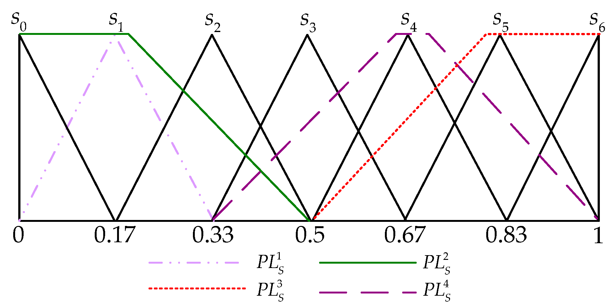
In the sequel, a numerical example is given to understand the aforesaid process of obtaining the fuzzy envelope for the PLTSs.

Example 2.

Let$S=\{s_0,s_1,\cdots ,s_6\}$be a linguistic term set with its triangular fuzzy membership function shown in Figure 2. In order to grasp the proposed fuzzy envelope determining approach, an example is conducted as follows:

• Fuzzy envelope for PLTS$P{L}_S^1=\{s_1(1)\}$can be obtained as$env(P{L}_S^1)=Tr(0,0.17,0.17,0.33)$.
• Fuzzy envelope for PLTS$P{L}_S^2=\{s_0(0.2),s_1(0.3),s_2(0.4)\}$is obtained as follows:
  $b_1=b_2=\min \{a_0^l,a_0^m,a_1^m,a_2^m,a_2^u\}=a_0^l=0$,$b_4=\max \{a_0^l,a_0^m,a_1^m,a_2^m,a_2^u\}=a_2^u=0.5$. Since$s_i=s_2$, according to [43], $\lambda =2/6$, then

  $$b_3=\frac{1}{\frac{2}{6}\times 0.4+\frac{2}{6}(1-\frac{2}{6})\times 0.3+{(1-\frac{2}{6})}^2\times 0.2}(\frac{2}{6}\times 0.4\times a_2^m+\frac{2}{6}(1-\frac{2}{6})\times 0.3\times a_1^m+{(1-\frac{2}{6})}^2\times 0.2\times a_0^m)=0.192.$$

  Therefore, $env(P{L}_S^2)=Tr(0,0,0.192,0.5)$.
• Fuzzy envelope for PLTS$P{L}_S^3=\{s_4(0.5),s_5(0.2),s_6(0.3)\}$is obtained as follows:
  $b_1=\min \{a_4^l,a_4^m,a_5^m,a_6^m,a_6^u\}=a_4^l=0.5$,$b_3=b_4=\max \{a_4^l,a_4^m,a_5^m,a_6^m,a_6^u\}=a_6^u=1$. Since$s_i=s_4$, according to [43], $\lambda =4/6$, then

  $$b_2=\frac{1}{{(\frac{4}{6})}^2\times 0.3+\frac{4}{6}(1-\frac{4}{6})\times 0.2+(1-\frac{4}{6})\times 0.5}({(\frac{4}{6})}^2\times 0.3\times a_6^m+\frac{4}{6}(1-\frac{4}{6})\times 0.2\times a_5^m+(1-\frac{4}{6})\times 0.5\times a_4^m)=0.818.$$

  Thus, $env(P{L}_S^3)=Tr(0.5,0.818,1,1)$.
• Fuzzy envelope for PLTS$P{L}_S^4=\{s_3(0.2),s_4(0.3),s_5(0.5)\}$is obtained as follows:
  $b_1=\min \{a_3^l,a_3^m,a_4^m,a_5^m,a_5^u\}=a_3^l=0.33$,$b_4=\max \{a_3^l,a_3^m,a_4^m,a_5^m,a_5^u\}=a_5^u=1$. Since$s_i=s_3$and$s_j=s_5$, according to [43], ${\lambda }_1=4/5$ (for determining $b_2$) and ${\lambda }_2=1/5$ (for determining $b_3$), then $b_2=\frac{1}{\frac{4}{5}\times 0.3+(1-\frac{4}{5})\times 0.2}(\frac{4}{5}\times 0.3\times a_4^m+(1-\frac{4}{5})\times 0.2\times a_3^m)=0.646$ and $b_3=\frac{1}{\frac{1}{5}\times 0.5+(1-\frac{1}{5})\times 0.3}(\frac{1}{5}\times 0.5\times a_5^m+(1-\frac{1}{5})\times 0.3\times a_4^m)=0.717$.

Thus,$env(P{L}_S^4)=Tr(0.33,0.646,0.717,1)$.

The fuzzy envelopes obtained above are shown inFigure 3.

When the probabilities of all linguistic terms in $P{L}_S^i$ $(i=2,3,4)$ are equal and continue, then $P{L}_S^i$ $(i=2,3,4)$ can be regarded as the hesitant fuzzy linguistic term sets (HFLTSs). In this case, the fuzzy envelopes for $P{L}_S^i$ $(i=2,3,4)$ are exactly the same as those presented in [43], namely, $env(P{L}_S^2)=Tr(0,0,0.15,0.5)$, $env(P{L}_S^3)=Tr(0.5,0.85,1,1)$ and $env(P{L}_S^4)=Tr(0.33,0.64,0.7,1)$.

Hence, the approach to determining the fuzzy envelope for PLTS proposed by this paper can generalize that proposed by [43], which shows the effectiveness and flexibility of the proposed approach.

4.3. A New Cosine Similarity Measure for PLTSs

Currently, the cosine similarity measure has received popular attention in retrieving information and collecting data. Liao and Xu [44] defined a cosine similarity measure for HFLTSs, as shown in Definition 9.

Definition 9

([44]). Let $S^{\prime }=\{s_{-\tau },\cdots ,s_{-1},s_0,s_1,\cdots ,s_{\tau }\}$ be a subscript-symmetric linguistic term set. Given any two HFLTSs $H_{S^{\prime }}^i=\left\{s_{{\gamma }_l^i}\right|s_{{\gamma }_l^i}\in S^{\prime },l=1,2,\cdots ,\#H_{S^{\prime }}^i\}$ $(i=1,2)$, the cosine similarity measure between them is formulated as

$$S_{\cos }(H_{S^{\prime }}^1,H_{S^{\prime }}^2)=\frac{{\displaystyle {\sum }_{l=1}^{\#H_{S^{\prime }}}\frac{\left|{\gamma }_l^1\right|}{2\tau +1}\cdot \frac{\left|{\gamma }_l^2\right|}{2\tau +1}}}{\sqrt{{\displaystyle {\sum }_{l=1}^{\#H_{S^{\prime }}}{(\frac{\left|{\gamma }_l^1\right|}{2\tau +1})}^2{\displaystyle {\sum }_{l=1}^{\#H_{S^{\prime }}}(\frac{\left|{\gamma }_l^2\right|}{2\tau +1}}{)}^2}}}$$

(10)

where $\#H_{S^{\prime }}=\max \{\#H_{S^{\prime }}^1,\#H_{S^{\prime }}^2\}$. If $\#H_{S^{\prime }}^1>\#H_{S^{\prime }}^2$, $H_{S^{\prime }}^2$ should be converted to a new one with the same length as $\#H_{S^{\prime }}^1$ by adding the smallest ones in $H_{S^{\prime }}^2$ and the probabilities of them are zero.

Inspired by Definition 9 and according to the fuzzy envelopes for PLTSs, the cosine similarity measure for PLTSs is defined as follows.

Definition 10.

Let$P{L}_S^i$$(i=1,2)$be any two PLTSs and$env(P{L}_S^i)=Tr(b_{i1},b_{i2},b_{i3},b_{i4})$$(i=1,2)$be their fuzzy envelopes. The cosine similarity measure between$P{L}_S^1$and$P{L}_S^2$is formulated as

$$S_{\cos }(P{L}_S^1,P{L}_S^2)=\frac{{\displaystyle {\sum }_{k=1}^4{b}_{1k}{b}_{2k}}}{\sqrt{{\displaystyle {\sum }_{k=1}^4{(b_{1k})}^2}{\displaystyle {\sum }_{k=1}^4{(b_{2k})}^2}}}$$

(11)

According to the relationship between distance and similarity measure mentioned in [44], the corresponding cosine distance measure can be defined as

$$d_{\cos }(P{L}_S^1,P{L}_S^2)=1-S_{\cos }(P{L}_S^1,P{L}_S^2)=1-\frac{{\displaystyle {\sum }_{k=1}^4{b}_{1k}{b}_{2k}}}{\sqrt{{\displaystyle {\sum }_{k=1}^4{(b_{1k})}^2}{\displaystyle {\sum }_{k=1}^4{(b_{2k})}^2}}}$$

(12)

The above Equations (11) and (12) satisfy boundness (i.e., $0\le S_{\cos }(P{L}_S^1,P{L}_S^2)\le 1$) and reflexivity (i.e., $S_{\cos }(P{L}_S^1,P{L}_S^2)=S_{\cos }(P{L}_S^2,P{L}_S^1)$). Generally, the greater the cosine similarity measure between two PLTSs, the more analogous they are, and the smaller the distance.

Based on the relative repetition degree and the diversity degree of probabilities for linguistic terms, Xian et al. [25] proposed a similarity measure for PLTSs. In order to compare with the similarity measure defined in [25], a numerical example is given as follows.

Example 3.

Let$P{L}_S^1=\{s_5(1)\}$,$P{L}_S^2=\{s_3(0.1),s_4(0.4),s_5(0.5)\}$and$P{L}_S^3=\{s_4(0.4),s_5(0.5),s_6(0.1)\}$be three PLTSs. Their fuzzy envelopes can be calculated as$env(P{L}_S^1)=Tr(0.67,0.83,0.83,1)$,$env(P{L}_S^2)=Tr(0.33,0.66,0.708,1)$and$env(P{L}_S^3)=Tr(0.5,0.782,1,1)$. Then, in the light of Equation (11), the cosine similarity measures between them can be computed as$S_{\cos }(P{L}_S^1,P{L}_S^2)=0.98$and$S_{\cos }(P{L}_S^1,P{L}_S^3)=0.99$. By using the formula of Xian et al. [24], it can be calculated that $S_{\cos }(P{L}_S^1,P{L}_S^2)=S_{\cos }(P{L}_S^1,PL{H}_S^3)=0.861$.

Due to the fact that $s_6$ is closer to $s_5$ than $s_3$, it is more in line with humanintuition that the similarity between $P{L}_S^1$ and $P{L}_S^3$ is higher than that between $P{L}_S^1$ and $P{L}_S^2$. In addition, it was mentioned that there is no need to normalize the PLTSs when determining their fuzzy envelopes. Thus, the proposed similarity measure has strong ability to preserve more initial information from the PLTSs. Nevertheless, it is necessary to normalize the PLTSs when using the similarity measure of Xian et al. [25]. Hence, the similarity measure proposed in this paper is more reasonable than the one proposed in [25].

5. A Probabilistic Linguistic Matrix Game Based on Fuzzy Envelope and PT

In this section, a probabilistic linguistic matrix game (PLMG) is formulated. Afterwards, based on fuzzy envelope and considering the player’s psychological behavior, an effective method is developed to solve the PLMG. The framework of the proposed method is also presented.

5.1. Model Formulation

Due to the fact that PLTSs have the strong ability to describe uncertain and imprecise payoff values, the formal description of the PLMG is given to construct the programming models. In this PLMG, the pure strategy spaces of players $P_I$ and $P_{II}$ are denoted as $S_{P_I}=\{{\xi }_1,{\xi }_2,\cdots ,{\xi }_r\}$ and $S_{P_{II}}=\{{\varsigma }_1,{\varsigma }_2,\cdots ,{\varsigma }_t\}$, respectively. The vectors $\mathit{y}={(y_1,y_2,\cdots ,y_r)}^{{\rm T}}$ and $\mathit{z}={(z_1,z_2,\cdots ,z_t)}^{{\rm T}}$ are the mixed strategies of players $P_I$ and $P_{II}$, where the $y_i(i=1,2,\cdots ,r)$ and $z_j(j=1,2,\cdots ,t)$ are the probabilities for players $P_I$ and $P_{II}$ that choose pure strategies ${\xi }_i\in S_{P_I}(i=1,2,\cdots ,r)$ and ${\varsigma }_j\in S_{P_{II}}(j=1,2,\cdots ,t)$, separately. The mixed strategy spaces for player $P_I$ is $Y=\left\{\mathit{y}\right|{\displaystyle {\sum }_{i=1}^r{y}_i}=1,y_i\ge 0\}$ and the mixed strategy spaces for player $P_{II}$ is $Z=\left\{\mathit{z}\right|{\displaystyle {\sum }_{j=1}^t{z}_j}=1,z_j\ge 0\}$. Suppose that the player $P_I$ takes the pure strategy ${\xi }_i$ to maximize his/her benefit, and the player $P_{II}$ selects the pure strategy ${\varsigma }_j$ to minimize his/her loss (i.e., at situation $({\xi }_i,{\varsigma }_j)$), the profit of player $P_I$ is $P{L}_S^{ij}$, where $P{L}_S^{ij}$ is a PLTS defined in Definition 4. Let $S=(s_0,s_1,\cdots ,s_{\tau })$ be a linguistic term set. For simplicity, the payoff matrix of PLMG is denoted as ${\tilde{P}}_L={(P{L}_S^{ij})}_{r\times t}$, which can be described as

$$\begin{array}{ll}& \begin{array}{cccc}{\varsigma }_1& {\varsigma }_2& \cdots & {\varsigma }_t\end{array}\\ {\tilde{P}}_L=\begin{array}{c}{\xi }_1\\ {\xi }_2\\ ⋮\\ {\xi }_r\end{array}& \left(\begin{array}{cccc}P{L}_S^{11}& P{L}_S^{12}& \cdots & P{L}_S^{1t}\\ P{L}_S^{21}& P{L}_S^{22}& \cdots & P{L}_S^{2t}\\ ⋮& ⋮& & ⋮\\ P{L}_S^{r1}& P{L}_S^{r2}& \cdots & P{L}_S^{rt}\end{array}\right)\end{array}$$

Hereinafter, the PLMG with mixed strategies is abbreviated as $(S_{P_I},X;S_{P_{II}},Y;{\tilde{P}}_L)$.

If players $P_I$ and $P_{II}$ take any mixed strategies $\mathit{y}\in Y$ and $\mathit{z}\in Z$, then the expected payoff of player $P_I$ is $\tilde{E}(\mathit{y},\mathit{z})={\mathit{y}}^T{\tilde{P}}_L\mathit{z}={\displaystyle \sum _{i=1}^r{\displaystyle \sum _{j=1}^t{y}_{i}P{L}_S^{ij}{z}_j}}=\{{\displaystyle \sum _{i=1}^r{\displaystyle \sum _{j=1}^t{y}_i{s}_{(1)}^{ij}(p_{(1)}^{ij})z_j}},$ ${\displaystyle \sum _{i=1}^r{\displaystyle \sum _{j=1}^t{y}_i{s}_{(2)}^{ij}(p_{(2)}^{ij})z_j}},\cdots ,{\displaystyle \sum _{i=1}^r{\displaystyle \sum _{j=1}^t{y}_i{s}_{(\#P{L}_S)}^{ij}(p_{(\#P{L}_S)}^{ij})z_j}}\}$, where $\#P{L}_S$ is the length of $P{L}_S^{ij}$.

Let $P_I$ be the maximize player, $P_{II}$ be the minimize player. From the perspective of gain-floor and loss-ceiling, the goals of players $P_I$ and $P_{II}$ can be constructed as follows, respectively.

Player $P_I$: $\underset{y\in Y}{\max }\underset{z\in Z}{\min }{\mathit{y}}^T{\tilde{P}}_L\mathit{z}$ and player $P_{II}$: $\underset{z\in Z}{\min }\underset{y\in Y}{\max }{\mathit{y}}^T{\tilde{P}}_L\mathit{z}$.

Let $\tilde{U}$ represent the minimal fuzzy payoff value of player $P_I$ and $\tilde{V}$ represent the maximal fuzzy payoff value of player $P_{II}$ [5]. The goals of players can be transformed as ${\mathit{y}}^T{\tilde{P}}_L\tilde{\ge }\tilde{U}$ for each strategy $\mathit{y}\in Y$ and ${\tilde{P}}_L\mathit{z}\tilde{\le }\tilde{V}$ for each strategy $\mathit{z}\in Z$. The symbols “$\tilde{\ge }$” and “$\tilde{\le }$” are the probabilistic linguistic version of the crisp order relation, meaning “essentially not less than” and “essentially not larger than”, respectively. Now, to get the maximin strategy ${\mathit{y}}^{\ast }$ and the minimax strategy ${\mathit{z}}^{\ast }$, the following two fuzzy programming models have to be solved.

$$\begin{array}{ll}& \max \tilde{U}\\ s.t.& \{\begin{array}{l}{\displaystyle {\sum }_{i=1}^{r}P{L}_S^{ij}{y}_i}\tilde{\ge }\tilde{U},(j=1,2,\cdots ,t)\\ {\displaystyle {\sum }_{i=1}^r{y}_i}=1,y_i\ge 0,(i=1,2,\cdots ,r)\end{array}\end{array}$$

(13)

and

$$\begin{array}{ll}& \min \tilde{V}\\ s.t.& \{\begin{array}{l}{\displaystyle {\sum }_{j=1}^{t}P{L}_S^{ij}{z}_j}\tilde{\le }\tilde{V},(i=1,2,\cdots ,r)\\ {\displaystyle {\sum }_{j=1}^t{z}_j}=1,z_j\ge 0,(j=1,2,\cdots ,t)\end{array}\end{array}$$

(14)

5.2. Solving the Models

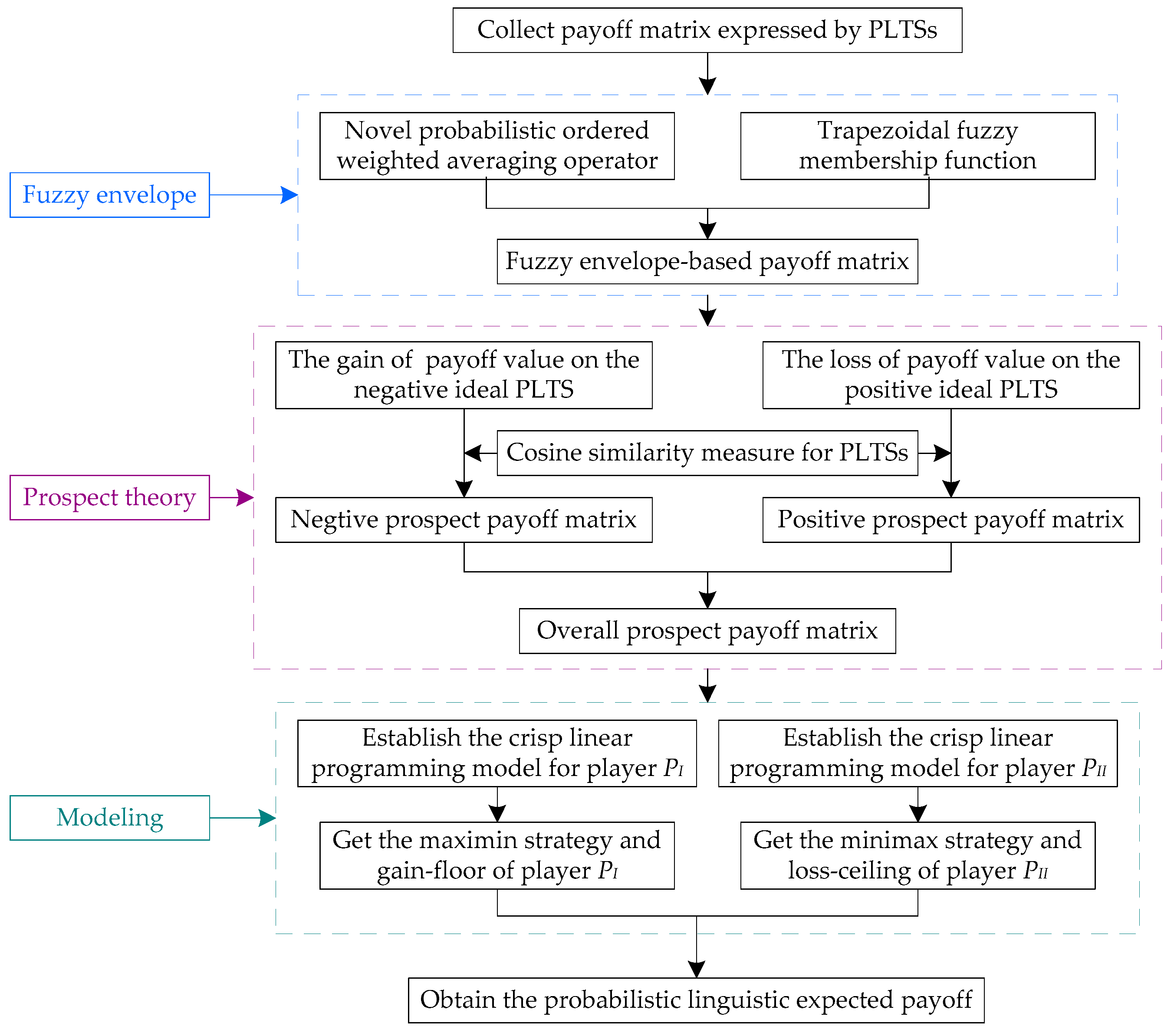
Since the payoff values $P{L}_S^{ij}$ in the payoff matrix $P_L$ are expressed by PLTSs, the traditional method failed to address the aforesaid game models. In this paper, a new method is developed to find the optimal solution for the mathematical models. Firstly, by using the approach presented in Section 4.2, all elements in the probabilistic linguistic payoff matrix are represented by trapezoidal fuzzy membership function and a fuzzy envelope-based payoff matrix is formed. Then, considering DMs’ psychological behavior, the fuzzy envelope-based payoff matrix is transformed into an overall prospect payoff matrix through applying PT. Finally, based on the prospect payoff matrix, two linear programming models are constructed and solved.

Now, the specific and detailed processes for seeking the maximin and the minimax strategies are profiled as follows:

Step 1. Convert the probabilistic linguistic payoff matrix ${\tilde{P}}_L={(P{L}_S^{ij})}_{r\times t}$ into the fuzzy envelope-based payoff matrix ${\tilde{F}}_{env}={(T{r}_{ij})}_{r\times t}$, where $T{r}_{ij}=Tr(b_{ij}^1,b_{ij}^2,b_{ij}^3,b_{ij}^4)$ $(i=1,2,\cdots ,r;j=1,2,\cdots t)$.

By using the technique presented in Section 4.2, the entire elements in the probabilistic linguistic payoff matrix can be represented by their trapezoidal fuzzy membership functions. As a result, the fuzzy envelope-based payoff matrix ${\tilde{F}}_{env}={(T{r}_{ij})}_{r\times t}$ can be obtained.

Step 2. Transform the fuzzy envelope-based payoff matrix into a prospect payoff matrix through the application of PT.

(i)

Define the reference point

The choice of reference point is the key and also the core of PT. When making a decision, the DM will measure the gain or loss on the basis of the reference point. The selection of the preference point is frequently dependent on the risk attitude and psychological behavior of DMs [34]. In this paper, the positive ideal point and the negative ideal point are taken as the double reference points. Suppose that the positive and negative ideal PLTSs are $T{r}^{+}=\{s_{\tau }(1)\}=Tr(b_1^{+},b_2^{+},b_3^{+},b_4^{+})$ and $T{r}^{-}=\{s_0(1)\}=Tr(b_1^{-},b_2^{-},b_3^{-},b_4^{-})$, respectively.

(ii)

Calculate the gain and loss of $T{r}_{ij}$ on the negative and positive ideal PLTS

To characterize the “utility value” that the player perceives in gain and the “regret value” that the player perceives in loss, the cosine distance between $T{r}_{ij}$ and the negative ideal PLTS is deemed as the gain and the cosine distance between $T{r}_{ij}$ and the positive ideal PLTS is viewed as the loss.

According to Definition 10, the gain of $T{r}_{ij}$ on the negative ideal PLTS $T{r}^{-}=\{s_0(1)\}=Tr(b_1^{-},b_2^{-},b_3^{-},b_4^{-})$ is given as

$$d_{\cos }(T{r}_{ij},T{r}^{-})=1-S_{\cos }(T{r}_{ij},T{r}^{-})=1-\frac{{\displaystyle {\sum }_{k=1}^4{b}_{ij}^k{b}_k^{-}}}{\sqrt{{\displaystyle {\sum }_{k=1}^4{(b_{ij}^k)}^2}\times {\displaystyle {\sum }_{k=1}^4{(b_k^{-})}^2}}}$$

(15)

Similarity, the loss of $T{r}_{ij}$ on the positive ideal PLTS $T{r}^{+}=\{s_{\tau }(1)\}=Tr(b_1^{+},b_2^{+},b_3^{+},b_4^{+})$ is given as

$$d_{\cos }(T{r}_{ij},T{r}^{+})=1-S_{\cos }(T{r}_{ij},T{r}^{+})=1-\frac{{\displaystyle {\sum }_{k=1}^4{b}_{ij}^k{b}_k^{+}}}{\sqrt{{\displaystyle {\sum }_{k=1}^4{(b_{ij}^k)}^2}\times {\displaystyle {\sum }_{k=1}^4{(b_k^{+})}^2}}}$$

(16)

(iii)

Compute the overall prospect value of payoff value at situation $({\xi }_i,{\varsigma }_j)$ given by player $P_I$

In the view of Equation (4), the negative and positive prospect value of payoff value at situation $({\xi }_i,{\varsigma }_j)$ given by player $P_I$ on $T{r}^{-}$ and $T{r}^{+}$ can be obtained as

$$v_{ij}^{-}={(d_{\cos }(T{r}_{ij},T{r}^{-}))}^{\varphi }$$

(17)

$$v_{ij}^{+}=-\epsilon {(d_{\cos }(T{r}_{ij},T{r}^{+}))}^{\phi }$$

(18)

Therefore, the overall prospect value of payoff value at situation $({\xi }_i,{\varsigma }_j)$ given by player $P_I$ can be obtained as

$$v_{ij}=\eta v_{ij}^{-}+(1-\eta )v_{ij}^{+}$$

(19)

where the risk attitude parameter $\eta$ $(0\le \eta \le 1)$ indicates the different importance degrees of the positive and negative ideal PLTSs.

Step 3. The acquired overall prospect payoff matrix $v={(v_{ij})}_{r\times t}$ is considered as the crisp equivalent of the given payoff matrix ${\tilde{P}}_L={(P{L}_S^{ij})}_{r\times t}$. Now Equations (13) and (14) are turned into the following two crisp linear programming models, respectively.

$$\begin{array}{ll}& \max U\\ s.t.& \{\begin{array}{l}{\displaystyle {\sum }_{i=1}^r{v}_{ij}{y}_i}\ge U,(j=1,2,\cdots ,t)\\ {\displaystyle {\sum }_{i=1}^r{y}_i}=1,y_i\ge 0,(i=1,2,\cdots ,r)\end{array}\end{array}$$

(20)

$$\begin{array}{ll}& \min V\\ s.t.& \{\begin{array}{l}{\displaystyle {\sum }_{j=1}^t{v}_{ij}{z}_j}\le V,(i=1,2,\cdots ,r)\\ {\displaystyle {\sum }_{j=1}^t{z}_j}=1,z_j\ge 0,(j=1,2,\cdots ,t)\end{array}\end{array}$$

(21)

where $U$ and $V$ represent the crisp equivalents of gain-floor and loss-ceiling for players, respectively.

Step 4. Via solving the aforementioned two linear programming modelswith the ordinary simplex method, the maximin strategy ${\mathit{y}}^{\ast }$ for player $P_I$ and the minimax strategy ${\mathit{z}}^{\ast }$ for player $P_{II}$ can be acquired. In addition, the optimal crisp equivalent of the gain-floor $U^{\ast }$ and loss-ceiling $V^{\ast }$ for players $P_I$ and $P_{II}$ are evaluated here, respectively.

Step 5. The aggregated expected payoff for player $P_I$ can be calculated by employing the basic operations of PLTS introduced in [22].

5.3. Framework

Up to now, this paper has completed the method of solving the matrix game with probabilistic linguistic information. The framework (Figure 4) is described below to clearly explain the logic and organizational structure of the proposed method.

6. Results

This section provides an example from the development strategy of SNNR to illustrate the applicability of the proposed method. Then, sensitivity analysis and comparative analyses are conducted to show the flexibility and superiorities of the proposed method.

6.1. An Example from the Development Strategy of SNNR

The Sanjiangyuan region (the headwater region of the Yangtze, Yellow and Lantsang rivers) is located in the hinterland of the Qinghai-Tibet Plateau, south of Qinghai Province. The region is called the “Water tower of China” and has an important water storage function [45]. The region is essential not only for ecological water supply and regulation services, but also for ecological services of biodiversity conservation [46]. However, the ecosystem in this region is fragile and the impact of climate change (especially global warming) on this region is particularly obvious [47]. Rapid population growth, unconstrained economic development and extensive human activities have enormously exacerbated the deterioration of the ecological environment, including the degradation of grassland, soil erosion and the loss of biodiversity [48]. In order to strengthen the ecological and environmental protection of this region, the Chinese government established the Sanjiangyuan National Nature Reserve (SNNR) in 2000 and launched the Sanjiangyuan ecological project in 2005 [49]. SNNR is the largest nature reserve in China covering an area of 363,000 square kilometers. The establishment of the nature reserve aims to safeguard and preserve the biodiversity and natural ecological balance of the region.

Nevertheless, as an underdeveloped region in China, the Sanjiangyuan region is facing a series of problems under the combined effects of global climate change and increasingly frequent human economic activities: the uncoordinated contradiction between humans and Nature is gradually becoming prominent; the ecological environment is deteriorating; the number of ecological refugees is increasing year by year; the contradiction between population, resources, environment and development is becoming more and more serious; the situation for ecological environment protection and natural resource development and utilization are becoming increasingly grim [50]. How to sustainably develop the economy and steadily improve peoples’ lives without destroying the local ecological environment is a difficult and urgent matter. Thus, it has highly significant academic value and practical application to research the interaction between economy and ecology in the Sanjiangyuan region, and formulate a development strategy for SNNR. In order to explore the balance between economic development and ecological protection, Xue et al. [6] have used a hesitant fuzzy matrix game method to study the development strategy of SNNR, considering that PLTSs have more powerful and flexible capabilities than HFLTSs in disposing of uncertain information, which is also more in line with human thinking. Therefore, this paper intends to apply the PLMG method to solve the development strategy of SNNR.

In fact, different development goals may conflict with each other when formulating the development strategy of SNNR. Compared with other objectives such as biodiversity, water storage capacity and conserving wetland areas, the management department that formulates the development strategy (hereinafter referred to as management department) of SNNR may pay more attention to the goal of economic return. However, Nature and the management department are contradictory in terms of economic returns. Thus, two competitors are formed–the management department and Nature. In this paper, the management department that formulates the development strategy of SNNR is regarded as player $P_I$ and Nature as player $P_{II}$. ${\xi }_1$: Forestry, ${\xi }_2$: Manufacturing, ${\xi }_3$: Tourism, ${\xi }_4$: Planting and ${\xi }_5$: Livestock farming are five economic development schemes devised by the management department for the economic development of SNNR. The five different schemes can be viewed as the five strategies of player $P_I$ in the game. In a similar way, ${\varsigma }_1$: Economic benefit, ${\varsigma }_2$: Biological diversity, ${\varsigma }_3$: Capacity of water storage and ${\varsigma }_4$: Lakes and wetland area are four objectives considered by Nature for the coordinated development of ecology and economy for SNNR. These four different objectives can be viewed as the four strategies of player $P_{II}$ in the game.

Let S = {s₀: extremely poor (EP), s₁: very poor (VP), s₂: poor (P), s₃: medium (M), s₄: good (G), s₅: very good (VG), s₆: extremely good (EG)}be a LTS. The payoff matrix values with probabilistic linguistic information are shown in

Table 1. Payoff matrix values with probabilistic linguistic information.

Payoff Values	${\mathit{\varsigma }}_1$	${\mathit{\varsigma }}_2$	${\mathit{\varsigma }}_3$	${\mathit{\varsigma }}_4$
${\xi }_1$	20%EP, 30%VP, 40%P	50%G, 20%VG, 30%EG	30%M, 50%G, 20%VG	VG
${\xi }_2$	10%M, 40%G, 50%VG	30%VP, 70%P	50%P, 10%M, 20%G	30%P, 40%M, 30%G
${\xi }_3$	P	40%G, 50%VG, 10%EG	10%G, 90%VG	10%VP, 30%P, 50%M
${\xi }_4$	10%G, 20%VG, 70%EG	20%M, 30%G, 30%VG	EG	40%G, 60%VG
${\xi }_5$	60%M, 40%G	M	40%P, 60%M	20%M, 80%G

. These evaluation values in the payoff matrix are given by the invited team of senior experts after field research, consulting relevant historical materials and combining the current national policies.

The evaluation information in Table 1 can be described in the forms of PLTSs in the probabilistic linguistic payoff matrix ${\tilde{P}}_L$.

$$\begin{array}{ll}& \begin{array}{cccc}{\varsigma }_1& {\varsigma }_2& {\varsigma }_3& {\varsigma }_4\end{array}\\ {\tilde{P}}_L=\begin{array}{c}{\xi }_1\\ {\xi }_2\\ {\xi }_3\\ {\xi }_4\\ {\xi }_5\end{array}& \left(\begin{array}{cccc}\{s_0(0.2),s_1(0.3),s_2(0.4)\}& \{s_4(0.5),s_5(0.2),s_6(0.3)\}& \{s_3(0.3),s_4(0.5),s_5(0.2)\}& \{s_5(1)\}\\ \{s_3(0.1),s_4(0.4),s_5(0.5)\}& \{s_1(0.3),s_2(0.7)\}& \{s_2(0.5),s_3(0.1),s_4(0.2)\}& \{s_2(0.3),s_3(0.4),s_4(0.3)\}\\ \{s_2(1)\}& \{s_4(0.4),s_5(0.5),s_6(0.1)\}& \{s_4(0.1),s_5(0.9)\}& \{s_1(0.1),s_2(0.3),s_3(0.5)\}\\ \{s_4(0.1),s_5(0.2),s_6(0.7)\}& \{s_3(0.2),s_4(0.3),s_5(0.3)\}& \{s_6(1)\}& \{s_4(0.4),s_5(0.6)\}\\ \{s_3(0.6),s_4(0.4)\}& \{s_3(1)\}& \{s_2(0.4),s_3(0.6)\}& \{s_3(0.2),s_4(0.8)\}\end{array}\right)\end{array}$$

6.2. Solving the Case by the Proposed Method

Step 1. Take the trapezoidal fuzzymembership function to represent the entire elements in probabilistic linguistic payoff matrix ${\tilde{P}}_L$. Then, a fuzzy envelope-based payoff matrix ${\tilde{F}}_{env}={(T{r}_{ij})}_{5\times 4}$ can be obtained through the approach introduced in Section 4.2.

$${\tilde{F}}_{evn}=\left(\begin{array}{cccc}Tr(0,0,0.192,0.5)& Tr(0.5,0.818,1,1)& Tr(0.33,0.648,0.685,1)& Tr(0.67,0.83,0.83,1)\\ Tr(0.33,0.66,0.708,1)& Tr(0,0.17,0.33,0.5)& Tr(0.17,0.406,0.557,0.83)& Tr(0.17,0.473,0.527,0.83)\\ Tr(0.17,0.33,0.33,0.5)& Tr(0.5,0.782,1,1)& Tr(0.5,0.67,0.83,1)& Tr(0,0.318,0.38,0.67)\\ Tr(0.5,0.952,1,1)& Tr(0.33,0.646,0.702,1)& Tr(0.83,1,1,1)& Tr(0.5,0.67,0.83,1)\\ Tr(0.33,0.5,0.67,0.83)& Tr(0.33,0.5,0.5,0.67)& Tr(0.17,0.33,0.5,0.67)& Tr(0.33,0.5,0.67,0.83)\end{array}\right)$$

Step 2. Determine the reference point.

Let $T{r}^{+}=\{s_6(1)\}=Tr(0.83,1,1,1)$ and $T{r}^{-}=\{s_0(1)\}=Tr(0,0,0,0.17)$ be the positive ideal PLTS and the negative ideal PLTS, respectively.

Step 3. The gain $d_{\cos }(T{r}_{ij},T{r}^{-})$ and loss $d_{\cos }(T{r}_{ij},T{r}^{+})$ can be computed by using Equations (15) and (16). Afterwards, the obtained calculation results can form two cosine distance matrices, separately.

$$d_{\cos }^{-}={(d_{\cos }(T{r}_{ij},T{r}^{-}))}_{5\times 4}=\left(\begin{array}{cccc}0.0665& 0.4147& 0.2925& 0.4052\\ 0.3008& 0.1971& 0.2401& 0.2483\\ 0.2905& 0.4088& 0.3529& 0.1960\\ 0.4371& 0.2962& 0.4793& 0.3529\\ 0.3216& 0.3486& 0.2675& 0.3216\end{array}\right)$$

and

$$d_{\cos }^{+}={(d_{\cos }(T{r}_{ij},T{r}^{+}))}_{5\times 4}=\left(\begin{array}{cccc}0.3273& 0.0148& 0.0398& 0.0040\\ 0.0383& 0.1639& 0.0780& 0.0706\\ 0.0388& 0.0160& 0.0178& 0.1453\\ 0.0133& 0.0393& 0.0000& 0.0178\\ 0.0323& 0.0159& 0.0659& 0.0323\end{array}\right)$$

Step 4. Based on Equations (17) and (18), the negative prospect value $v_{ij}^{-}$ and positive prospect value $v_{ij}^{+}$ can be computed. After that, the negative and the positive prospect matrices can be formed, respectively.

$$v^{-}={(v_{ij}^{-})}_{5\times 4}=\left(\begin{array}{cccc}0.0920& 0.4609& 0.3390& 0.4516\\ 0.3475& 0.2395& 0.2849& 0.2935\\ 0.3370& 0.4552& 0.3998& 0.2383\\ 0.4828& 0.3428& 0.5236& 0.3998\\ 0.3685& 0.3956& 0.3134& 0.3685\end{array}\right)$$

and

$$v^{+}={(v_{ij}^{+})}_{5\times 4}=\left(\begin{array}{cccc}-0.8421& -0.0552& -0.1318& -0.0176\\ -0.1275& -0.4582& -0.2384& -0.2183\\ -0.1289& -0.0591& -0.0650& -0.4120\\ -0.0501& -0.1303& 0.0000& -0.0650\\ -0.1096& -0.0589& -0.2054& -0.1096\end{array}\right)$$

Step 5. Set the risk attitude parameter $\eta =0.5$; the overall prospect value $v_{ij}$ can be obtained by Equation (19). Then, all the acquired overall prospect value can constitute an overall prospect matrix.

$$v={(v_{ij})}_{5\times 4}=\left(\begin{array}{cccc}-0.3750& 0.2029& 0.1036& 0.2170\\ 0.1100& -0.1094& 0.0233& 0.0376\\ 0.1040& 0.1980& 0.1674& -0.0868\\ 0.2163& 0.1062& 0.2618& 0.1674\\ 0.1294& 0.1683& 0.0540& 0.1294\end{array}\right)$$

Step 6. Now, to obtain the maximin strategy ${\mathit{y}}^{\ast }$ and the crisp equivalent of the gain-floor $U^{\ast }$ for player $P_I$, a crisp linear programming model can be constructed as follows in the light of Equation (20).

$$\begin{array}{ll}& \max U\\ s.t.& \{\begin{array}{l}-0.3750y_1+0.1100y_2+0.1040y_3+0.2163y_4+0.1294y_5\ge U\\ 0.2029y_1-0.1094y_2+0.1980y_3+0.1062y_4+0.1683y_5\ge U\\ 0.1036y_1+0.0233y_2+0.1674y_3+0.2618y_4+0.0540y_5\ge U\\ 0.2170y_1+0.0376y_2-0.0868y_3+0.1674y_4+0.1294y_5\ge U\\ {\displaystyle {\sum }_{i=1}^5{y}_i}=1,y_i\ge 0,(i=1,2,\cdots ,5)\end{array}\end{array}$$

(22)

Solving the above linear programming model, the maximin strategy and the crisp equivalent of the gain-floor of player $P_I$ (i.e., management department) are obtained as ${\mathit{y}}^{\ast }={(0.0406,0,0.0196,0.4153,0.5245)}^T$ and $U^{\ast }=0.1445$.

Step 7. To obtain the minimax strategy ${\mathit{z}}^{\ast }$ and the crisp equivalent of the loss-ceiling $V^{\ast }$ for player $P_{II}$, a crisp linear programming model can be established by utilizing Equation (21).

$$\begin{array}{ll}& \min V\\ s.t.& \{\begin{array}{l}-0.3750z_1+0.2029z_2+0.1036z_3+0.2170z_4\le V\\ 0.1100z_1-0.1094z_2+0.0233z_3+0.0376z_4\le V\\ 0.1040z_1+0.1980z_2+0.1674z_3-0.0868z_4\le V\\ 0.2163z_1+0.1062z_2+0.2618z_3+0.1674z_4\le V\\ 0.1294z_1+0.1683z_2+0.0540z_3+0.1294z_4\le V\\ {\displaystyle {\sum }_{j=1}^4{z}_j}=1,z_j\ge 0,(j=1,2,\cdots ,4)\end{array}\end{array}$$

(23)

Solving the above linear programming model, the minimax strategy and the crisp equivalent of the loss-ceiling of player $P_{II}$ (i.e., Nature) are obtained as ${\mathit{z}}^{\ast }={(0.0822,0.6408,0.1303,0.1467)}^T$ and $V^{\ast }=0.1445$.

Step 8. Calculate the expected payoff of player $P_I$.

By employing the normalized method and the basic operations of PLTSs (see [22]), the expected payoff is calculated as follows:

$$\begin{array}{ll}\mathrm{E}({\mathit{y}}^{\ast },{\mathit{z}}^{\ast })& ={\left(\begin{array}{l}0.0406\\ 0\\ 0.0196\\ 0.4153\\ 0.5245\end{array}\right)}^{{\rm T}}\left(\begin{array}{cccc}\{s_{0.8667},s_{0.3333},s_0\}& \{s_2,s_{1.8},s_1\}& \{s_2,s_1,s_{0.9}\}& \{s_5,s_0,s_0\}\\ \{s_{2.5},s_{1.6},s_{0.3}\}& \{s_{1.4},s_{0.3},s_0\}& \{s_{1.1333},s_{1.0667},s_{0.5}\}& \{s_{1.2},s_{1.2},s_{0.6}\}\\ \{s_2,s_0,s_0\}& \{s_{2.5},s_{1.6},s_{0.6}\}& \{s_{4.5},s_{0.4},s_0\}& \{s_{1.6},s_{0.6667},s_{0.1333}\}\\ \{s_{4.2},s_1,s_{0.4}\}& \{s_{1.8333},s_{1.4667},s_{0.8}\}& \{s_6,s_0,s_0\}& \{s_3,s_{1.6},s_0\}\\ \{s_{1.8},s_{1.6},s_0\}& \{s_3,s_0,s_0\}& \{s_{1.8},s_{0.8},s_0\}& \{s_{3.2},s_{0.6},s_0\}\end{array}\right)\left(\begin{array}{l}0.0822\\ 0.6408\\ 0.1303\\ 0.1467\end{array}\right)\\ & =\{s_{2.7398},s_{0.7681},s_{0.2653}\}\end{array}$$

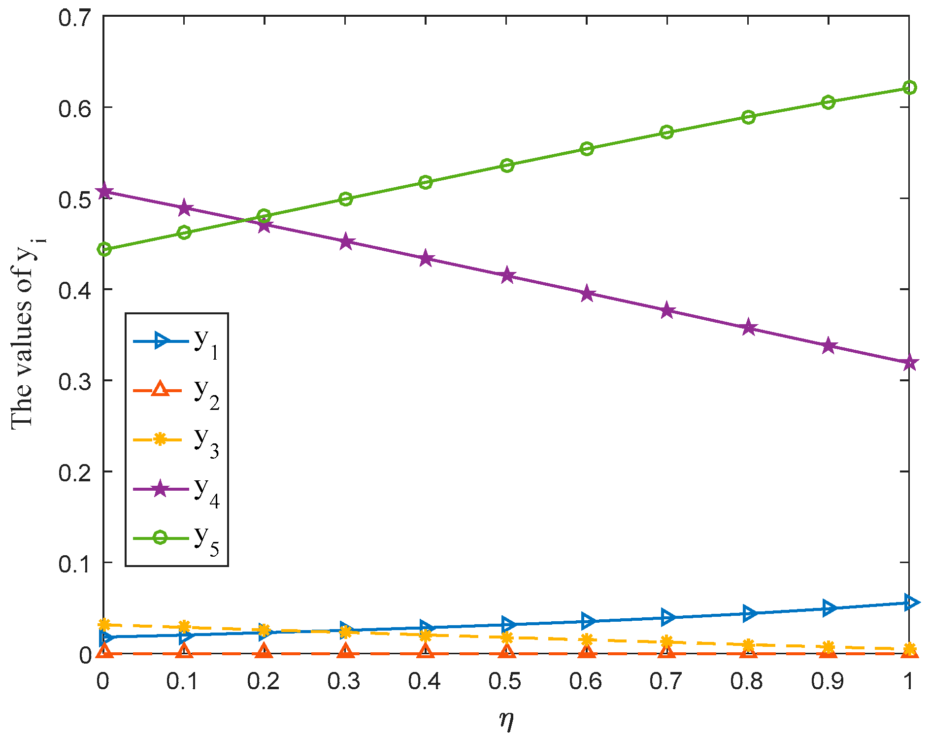
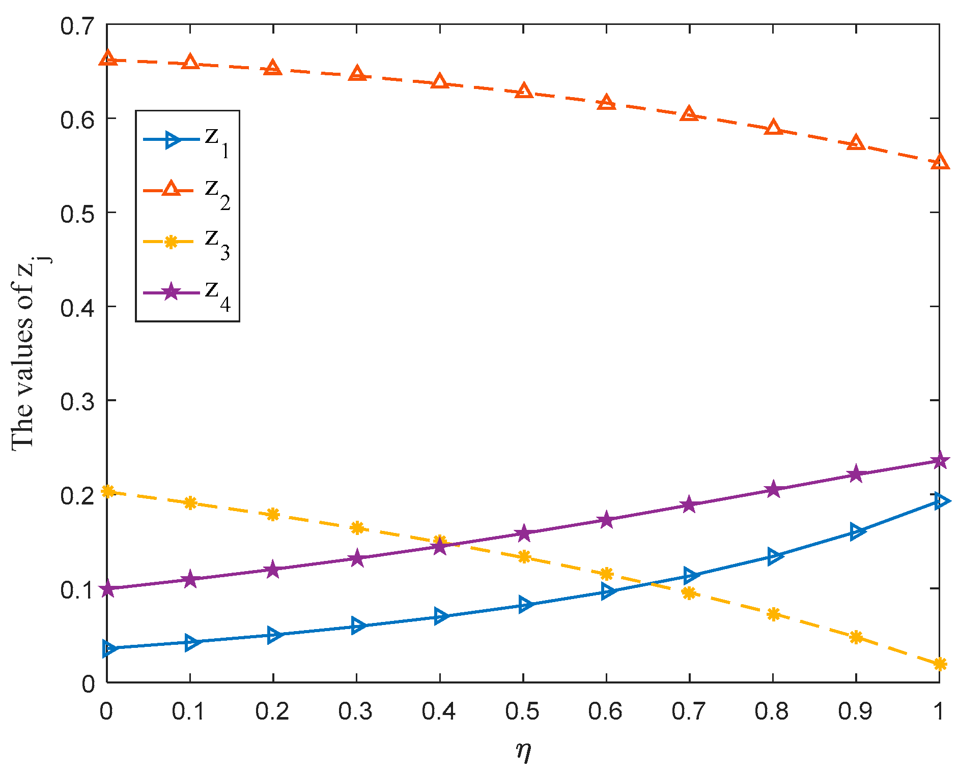
6.3. Sensitivity Analysis for the Parameter $\eta$

In Equation (19), the parameter $\eta$ ($0\le \eta \le 1$) is considered in the overall prospect value of payoff value at situation $({\xi }_i,{\varsigma }_j)$ given by player $P_I$. Then, this subsection adopts different values of parameter $\eta$ to solve the aforementioned case. The corresponding game results are shown in

Table 2. Optimal solutions of Equations (22) and (23) and the corresponding expected payoffs.

$\mathit{\eta }$	${\mathit{y}}^{\ast }$	${\mathit{z}}^{\ast }$	${\mathit{U}}^{*}$	${\mathit{V}}^{*}$	$\mathbf{E}({\mathit{y}}^{\ast },{\mathit{z}}^{\ast })$
0	${(0.0205,0,0.0330,0.5073,0.4392)}^T$	${(0.0353,0.6703,0.2029,0.0915)}^T$	−0.0951	−0.0951	$\{s_{2.7939},s_{0.7804},s_{0.3104}\}$
0.1	${(0.0239,0,0.0303,0.4892,0.4566)}^T$	${(0.0421,0.6665,0.1906,0.1007)}^T$	−0.0471	−0.0471	$\{s_{2.7809},s_{0.7759},s_{0.3017}\}$
0.2	${(0.0276,0,0.0276,0.4710,0.4738)}^T$	${(0.0499,0.6618,0.1774,0.1108)}^T$	0.0009	0.0009	$\{s_{2.7691},s_{0.7723},s_{0.2928}\}$
0.3	${(0.0316,0,0.0249,0.4525,0.4910)}^T$	${(0.0590,0.6560,0.1631,0.1218)}^T$	0.0488	0.0488	$\{s_{2.7583},s_{0.7695},s_{0.2838}\}$
0.4	${(0.0359,0,0.0222,0.4340,0.5079)}^T$	${(0.0696,0.6491,0.1475,0.1338)}^T$	0.0967	0.0967	$\{s_{2.7486},s_{0.7680},s_{0.2746}\}$
0.5	${(0.0406,0,0.0196,0.4153,0.5245)}^T$	${(0.0822,0.6408,0.1303,0.1467)}^T$	0.1445	0.1445	$\{s_{2.7398},s_{0.7681},s_{0.2653}\}$
0.6	${(0.0459,0,0.0170,0.3966,0.5405)}^T$	${(0.0972,0.6312,0.1111,0.1605)}^T$	0.1924	0.1924	$\{s_{2.7318},s_{0.7702},s_{0.2561}\}$
0.7	${(0.0518,0,0.0145,0.3779,0.5557)}^T$	${(0.1154,0.6200,0.0896,0.1750)}^T$	0.2402	0.2402	$\{s_{2.7241},s_{0.7750},s_{0.2469}\}$
0.8	${(0.0587,0,0.0122,0.3593,0.5699)}^T$	${(0.1377,0.6073,0.0650,0.1900)}^T$	0.2881	0.2881	$\{s_{2.7161},s_{0.7832},s_{0.2382}\}$
0.9	${(0.0668,0,0.0099,0.3410,0.5823)}^T$	${(0.1658,0.5931,0.0365,0.2046)}^T$	0.3360	0.3360	$\{s_{2.7065},s_{0.7961},s_{0.2300}\}$
1	${(0.0767,0,0.0078,0.3233,0.5923)}^T$	${(0.2022,0.5777,0.0026,0.2175)}^T$	0.3840	0.3840	$\{s_{2.6929},s_{0.8153},s_{0.2230}\}$

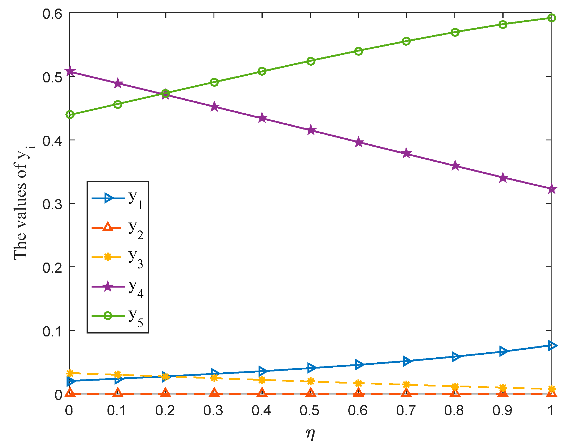
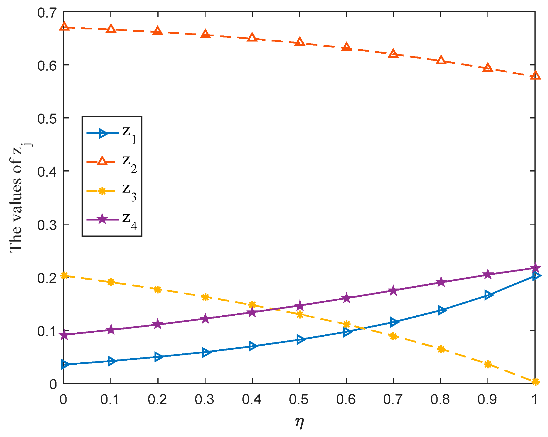
. Meanwhile, the optimal strategy ${\mathit{y}}^{\ast }$ and ${\mathit{z}}^{\ast }$ of players $P_I$ (management department) and $P_{II}$ (Nature) along with the variation tendencies of gain-floor and loss-ceiling of players $P_I$ and $P_{II}$ are drawn in Figure 5, Figure 6 and Figure 7 with $\eta$ varying from 0 to 1 at the interval 0.1.

• According to Table 2 and Figure 5, Figure 6 and Figure 7, we can receive the following observations:

  (i)

  The mixed strategies, gain-floor and loss-ceiling for players will change with the change of the parameter $\eta$, which reflects the flexibility of the proposed method.

  (ii)

  For the management department, when $\eta$ takes a value between 0.3 and 1, the probability ranking of each strategy in the selected mixed strategy keeps constant totally, that is, ${\xi }_5\ge {\xi }_4\ge {\xi }_1\ge {\xi }_3\ge {\xi }_2$. The stability of the probability ranking shows that the management department should put ${\xi }_5$: Livestock farming in the first place and ${\xi }_2$: Manufacturing should be the last consideration when formulating the development strategy for SNNR.

  (iii)

  For Nature, no matter how the parameter $\eta$ changes, Nature should put ${\varsigma }_2$: Biological diversity in first place since the probability of strategy ${\varsigma }_2$: Biological diversity in the selected mixed strategy is always greater than 0.5.

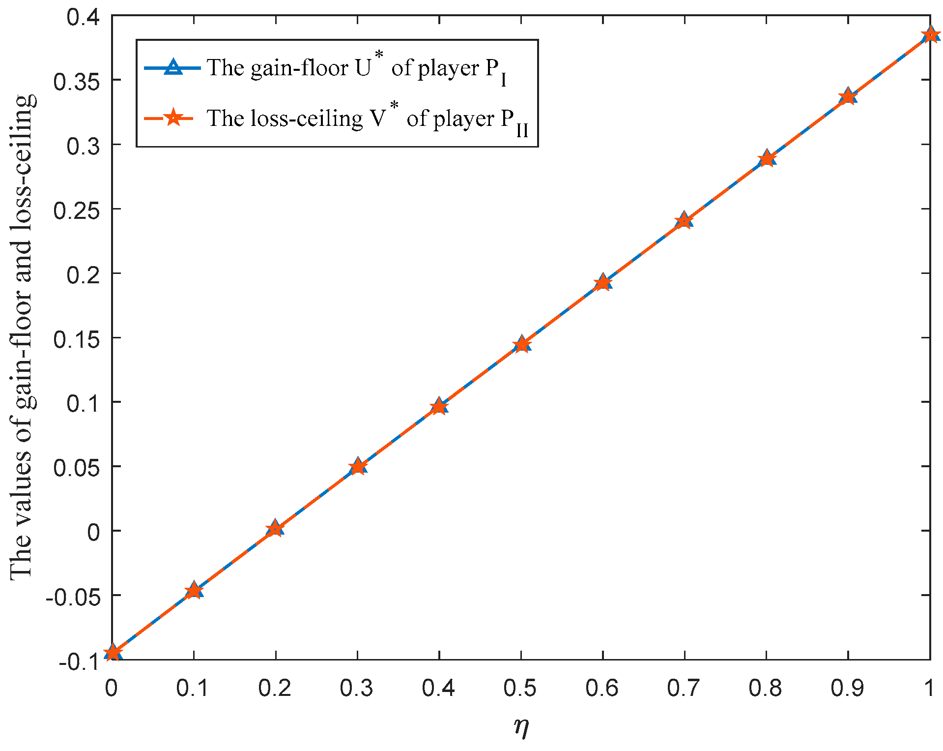
  (iv)

  The gain-floor and loss-ceiling for players are equal, whichis consistent with the results obtained in [13], and the values of these increase with the increase of the parameter $\eta$.

• Strategic interventions

In response to the development strategy of SNNR, it is recommended that the management department adopts a mixed strategy instead of a pure strategy. The management department is not to maximize short-term interests, but to pursue the sustainable development of human needs and Nature in the long term. Thus, it is impossible to reach the goal by relying on a single strategy. Using the information in the payoff matrix ${\tilde{P}}_L$, if the players believe that the positive ideal PLTS and negative ideal PLTS are of equal importance, then the management department is recommended to adopt a mixed strategy, namely, 4.06% Forestry, 1.96% Tourism, 41.53% Planting and 52.45% Livestock farming. If players believe that the importance of positive ideal PLTS and negative ideal PLTS is not equal, then the recommended strategy will be different. Besides, if the payoff matrix given by player changes, the optimal strategy obtained may also be different.

6.4. Comparative Analyses

6.4.1. Comparison with the Method without Considering Players’ Psychological Factor

This subsection compares the proposed method with the method [13] regardless of the players’ psychological behavior, which adopts the notion of composite relative similarity degree to the positive ideal fuzzy solution. To make the comparison fair, we implement the solution steps introduced in [13] on the basis of the trapezoidal fuzzy envelope matrix ${\tilde{F}}_{env}$, and the similarity degree adopts the cosine similarity degree defined in this paper. After a series of calculations, the final composite matrix $M$, which is regarded as the crisp equivalent of the payoff matrix ${\tilde{P}}_L$, is shown below.

$$M=\left(\begin{array}{cccc}0.1776& 0.2975& 0.2652& 0.3047\\ 0.2783& 0.2322& 0.2412& 0.2488\\ 0.2728& 0.2693& 0.2568& 0.2268\\ 0.2900& 0.2495& 0.2637& 0.2567\\ 0.2722& 0.2624& 0.2407& 0.2549\end{array}\right)$$

Based on the composite matrix $M$, Equations (20) and (21), two linear programming models can be constructed as follows:

$$\begin{array}{ll}& \max U_1\\ s.t.& \{\begin{array}{l}0.1776y_1+0.2783y_2+0.2728y_3+0.2900y_4+0.2722y_5\ge U_1\\ 0.2975y_1+0.2322y_2+0.2693y_3+0.2495y_4+0.2624y_5\ge U_1\\ 0.2652y_1+0.2412y_2+0.2568y_3+0.2637y_4+0.2407y_5\ge U_1\\ 0.3047y_1+0.2488y_2+0.2268y_3+0.2567y_4+0.2549y_5\ge U_1\\ {\displaystyle {\sum }_{i=1}^5{y}_i}=1,y_i\ge 0,(i=1,2,\cdots ,5)\end{array}\end{array}$$

(24)

and

$$\begin{array}{ll}& \min V_1\\ s.t.& \{\begin{array}{l}0.1776z_1+0.2975z_2+0.2652z_3+0.3047z_4\le V_1\\ 0.2783z_1+0.2322z_2+0.2412z_3+0.2488z_4\le V_1\\ 0.2728z_1+0.2693z_2+0.2568z_3+0.2268z_4\le V_1\\ 0.2900z_1+0.2495z_2+0.2637z_3+0.2567z_4\le V_1\\ 0.2722z_1+0.2624z_2+0.2407z_3+0.2549z_4\le V_1\\ {\displaystyle {\sum }_{j=1}^4{z}_j}=1,z_j\ge 0,(j=1,2,\cdots ,4)\end{array}\end{array}$$

(25)

By solving the above two models, the optimal solution can be obtained as: ${\mathit{y}}^{\ast }={(0.2183,0,0.1429,0.6321,0.0068)}^T$, ${\mathit{z}}^{\ast }={(0.2839,0.5053,0.0525,0.1582)}^T$, $U_1^{\ast }=V_1^{\ast }=0.2629$.

To stress the virtues of considering the psychological behavior of players, the results obtained by the proposed method (see Table 2 and Figure 5, Figure 6 and Figure 7) are compared with those obtained by the method [13]. The conclusions are summarized as follows:

• For player $P_I$, the probability ranking of each pure strategy in the selected mixed strategy ${\mathit{y}}^{\ast }={(0.2183,0,0.1429,0.6321,0.0068)}^T$ obtained by the method [13] is ${\xi }_4\ge {\xi }_1\ge {\xi }_3\ge {\xi }_5\ge {\xi }_2$, which is totally different from the probability ranking obtained by the proposed method (see Table 2 and Figure 5). That is to say, the probability ranking seems to change markedly if the game process does not include the psychological behavior of players. In addition, the probability of ${\xi }_5$: Livestock farming is largest when formulating the development strategy for SNNR, which is more in line with reality.
• For player $P_{II}$, the probability ranking of each pure strategy in the selected mixed strategy ${\mathit{z}}^{\ast }={(0.2839,0.5053,0.0525,0.1582)}^T$ obtained by the method [13] is ${\varsigma }_2\ge {\varsigma }_1\ge {\varsigma }_4\ge {\varsigma }_3$, which is slightly different from the probability ranking obtained by the proposed method (see Table 2 and Figure 6). Although the pure strategies with the largest probability obtained by the two methods are the same (i.e., ${\varsigma }_2$: Biological diversity), if the psychological behavior of the players without considering in the game process, the ranking of probability will change.
• According to Table 2 and Figure 7, the obtained gain-floor of player $P_I$ and the loss-ceiling of player $P_{II}$ by the method [13] are less than those that acquired by the proposed method when the parameter $\eta$ is not smaller than 0.8. Besides, the proposed method is also more flexible due to the consideration of players’ risk attitude.

Therefore, players’ psychological behavior will indeed have an impact on their optimal strategies. Specifically, players’ psychological behavior will change the ranking of the probability in the selected mixed strategy, resulting in different game results. This phenomenon is consistent with reality. Each player has different perception of gain and loss as a result of their psychological behavior, which will eventually change the game results. Thus, it is reasonable and necessary to incorporate players’ psychological behavior into the actual game process.

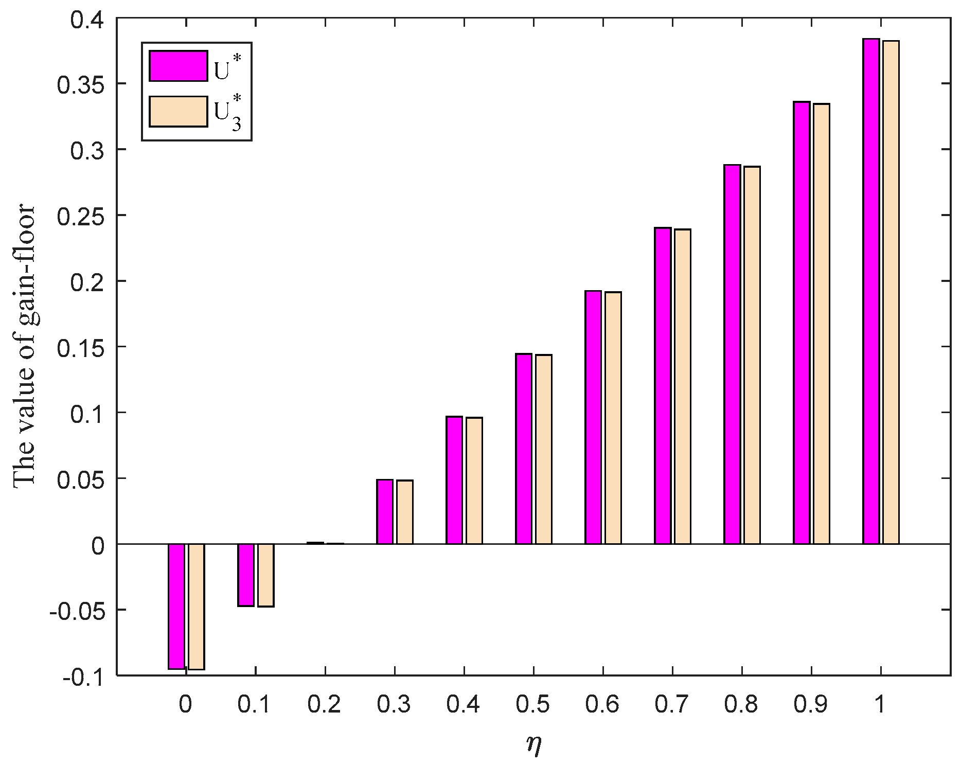
6.4.2. Comparison with Triangular Fuzzy Envelope

In order to highlight the advantages of trapezoidal fuzzy envelope used in this paper, this subsection first replaces the trapezoidal fuzzy membership function with the triangular membership function for PLTSs proposed by Mi et al. [5]. Then the proposed method is used to solve the aforesaid development strategy of SNNR. The calculation results are shown in

Table 3. Results obtained by using triangular fuzzy envelope for different values of $\eta$.

$\mathit{\eta }$	${\mathit{y}}^{\ast }$	${\mathit{z}}^{\ast }$	${\mathit{U}}_2^{*}$	${\mathit{V}}_2^{*}$
0	${(0.0595,0,0.0768,0.8637,0)}^T$	${(0.0643,0.9120,0,0.0236)}^T$	−0.0314	−0.0314
0.1	${(0.0726,0,0.0775,0.8500,0)}^T$	${(0.0706,0.9100,0,0.0194)}^T$	0.0067	0.0067
0.2	${(0.0861,0,0.0777,0.8362,0)}^T$	${(0.0771,0.9084,0,0.0145)}^T$	0.0448	0.0448
0.3	${(0.1002,0,0.0775,0.8224,0)}^T$	${(0.0837,0.9072,0,0.0090)}^T$	0.0830	0.0830
0.4	${(0.1148,0,0.0767,0.8085,0)}^T$	${(0.0906,0.9065,0,0.0029)}^T$	0.1212	0.1212
0.5	${(0.1772,0,0,0.8228,0)}^T$	${(0.0974,0.9026,0,0)}^T$	0.1595	0.1595
0.6	${(0.1931,0,0,0.8069,0)}^T$	${(0.1041,0.8959,0,0)}^T$	0.1979	0.1979
0.7	${(0.2093,0,0,0.7907,0)}^T$	${(0.1110,0.8890,0,0)}^T$	0.2363	0.2363
0.8	${(0.2258,0,0,0.7742,0)}^T$	${(0.1180,0.8820,0,0)}^T$	0.2749	0.2749
0.9	${(0.2426,0,0,0.7574,0)}^T$	${(0.1251,0.8749,0,0)}^T$	0.3134	0.3134
1	${(0.2598,0,0,0.7402,0)}^T$	${(0.1324,0.8676,0,0)}^T$	0.3521	0.3521

. Simultaneously, the optimal strategies ${\mathit{y}}^{\ast }$ and ${\mathit{z}}^{\ast }$ of players $P_I$ and $P_{II}$ with $\eta$ varying from 0 to 1 at the interval 0.1 are shown in Figure 8 and Figure 9, separately. Since the gain-floor of player $P_I$ and the loss-ceiling of player $P_{II}$ are equal invariably, the gain-floor $U_2^{\ast }$ and $U^{\ast }$ of player $P_I$ obtained by triangular fuzzy envelope and trapezoidal fuzzy envelope is plotted in Figure 10 only.

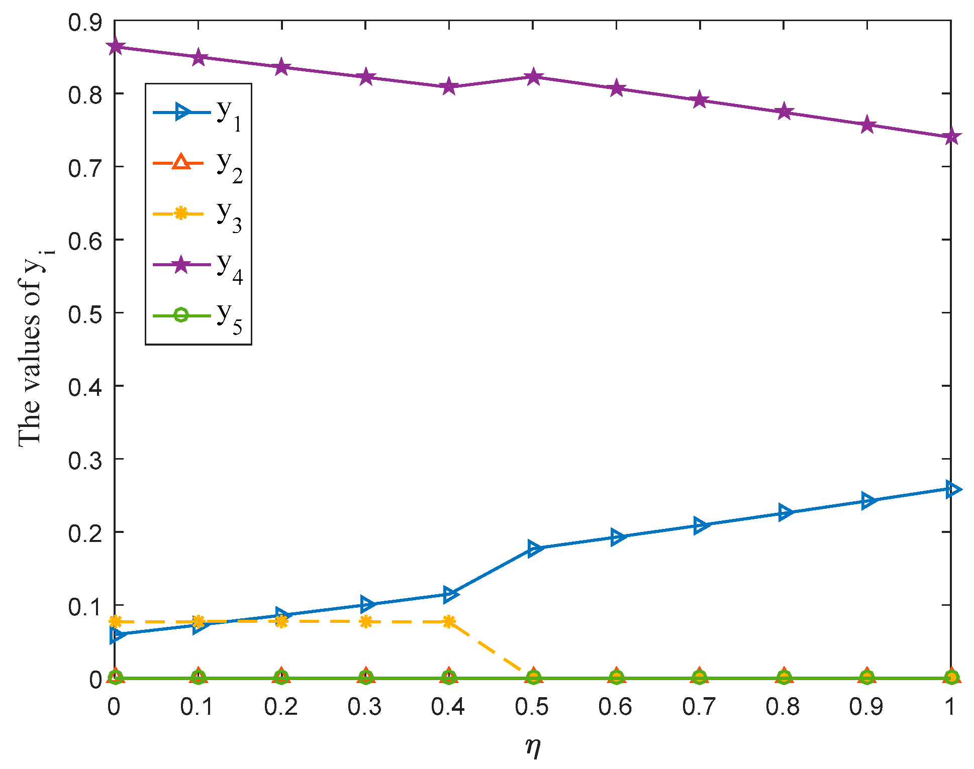
By comparing the results obtained by triangular fuzzy envelope method and trapezoidal fuzzy envelope method, the conclusions are summarized as follows:

• It can be seen from Table 3 and Figure 8 that the probability ranking obtained by the triangular fuzzy envelope method is completely different from that obtained by trapezoidal fuzzy envelope method. Moreover, the pure strategy with the highest probability is ${\xi }_4$: Planting, and the probabilities of selecting pure strategies ${\xi }_2$: Manufacturing and ${\xi }_5$: Livestock farming are equal to 0. The probability of ${\xi }_3$: Tourism is also equal to 0 when the parameter $\eta \ge 0.5$, which appears to be inconsistent with reality.
• According to Table 3 and Figure 9, the probability ranking of each pure strategy in the selected mixed strategy ${\mathit{z}}^{\ast }$ is ${\varsigma }_2>{\varsigma }_1>{\varsigma }_4>{\varsigma }_3$ when $\eta <0.5$. The probability ranking is ${\varsigma }_2>{\varsigma }_1>{\varsigma }_4={\varsigma }_3$ when $\eta \ge 0.5$. The pure strategies with the largest probability obtained by the two methods are ${\varsigma }_2$: Biological diversity, which is in line with the concept of sustainable development. However, as shown in Figure 9, the probability of selecting pure strategy ${\varsigma }_3$: Capacity of water storage is always equal to 0 no matter how the parameter $\eta$ changes, and the probability of ${\varsigma }_4$: Lakes and wetland area is also equal to 0 when $\eta \ge 0.5$, which does not conform to the actual situation evidently.
• In the light of Table 3 and Figure 10, we can find that when $\eta$ varies from 0 to 1, the variation tendency of the gain-floor $U_2^{\ast }$ of player $P_I$ obtained by the triangular fuzzy envelope method [5] is consistent with that obtained by the proposed method in this paper. However, when $0\le \eta \le 0.6$, the gain-floor $U^{\ast }$ (loss-ceiling $V^{\ast }$) is smaller than the gain-floor $U_2^{\ast }$ (loss-ceiling $V_2^{\ast }$). When $0.7\le \eta \le 1$, the gain-floor $U^{\ast }$ is greater than the gain-floor $U_2^{\ast }$. As mentioned earlier, the larger the value of the parameter $\eta$, the more optimistic the player, the better the result will be, that is, the greater the gain-floor and loss-ceiling. In reality, most players usually tend to ponder and solve the problem with an optimistic attitude. Hence, the greater the value of $\eta$, the higher the importance of the negative ideal PLTS, and the result obtained by the proposed method is better than the triangular fuzzy envelope method. The proposed method is more applicable for a situation in which the players are optimistic.

Thus, compared with triangular fuzzy envelope, the trapezoidal fuzzy envelope can grasp players’ evaluation information more comprehensively, and describe players’ judgments more accurately. The trapezoidal fuzzy envelope is used to flexibly deal with the linguistic information, which can make the game results more reliable.

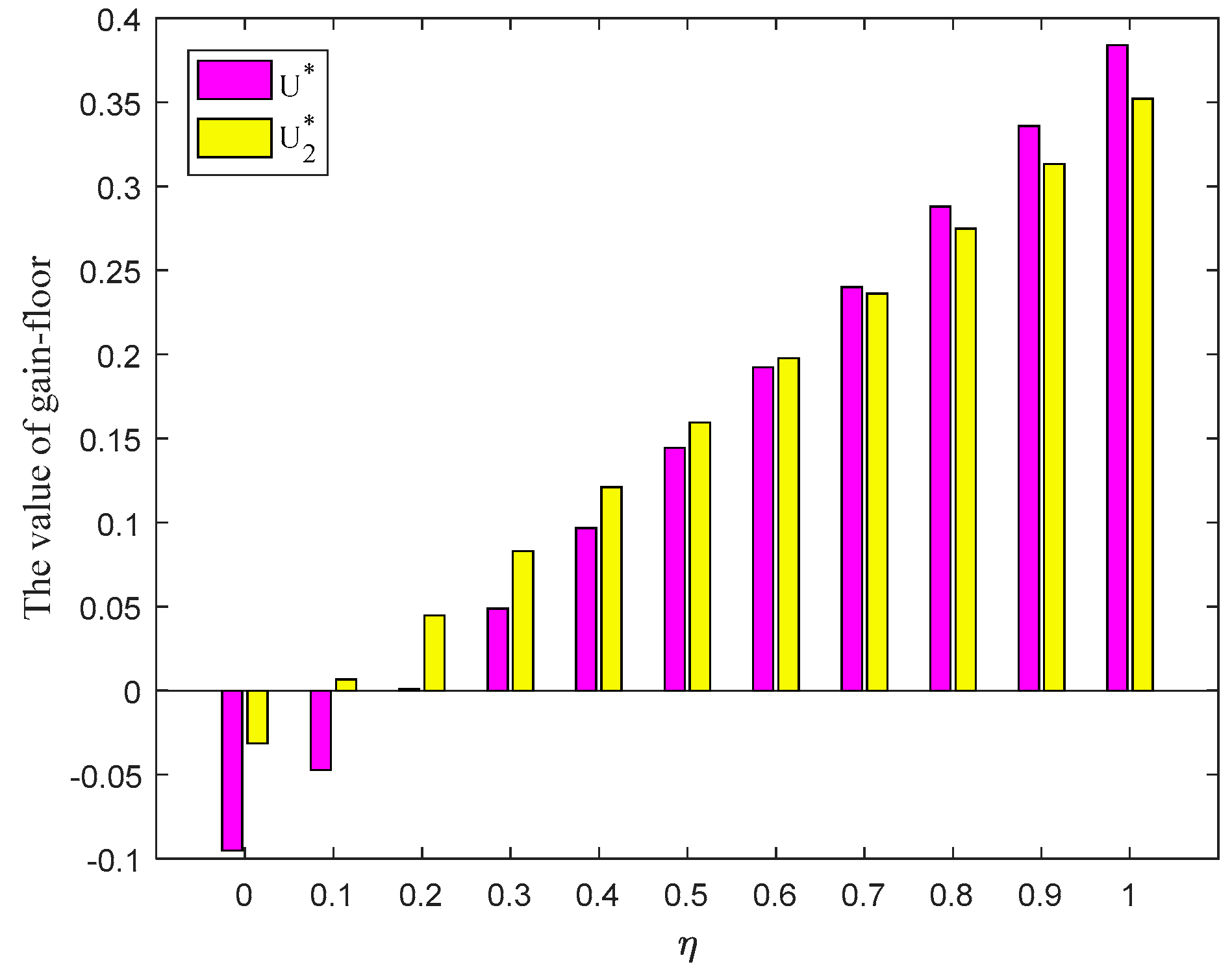
6.4.3. Comparison with Hesitant Fuzzy Linguistic Information

If we get rid of the probabilities from PLTSs, then the PLTSs are transformed into the HFLTSs. In order to emphasize the merits of using probabilistic linguistic information in this paper, this subsection first directly removes the probabilities behind all linguistic terms in the payoff matrix ${\tilde{P}}_L$, and then the HFLTSs are represented by their fuzzy envelope by using the method proposed in [43]; the subsequent solution steps are the same as those developed in this paper. The results are shown in

Table 4. Results obtained by hesitant fuzzy linguistic information for different values of $\eta$.

$\mathit{\eta }$	${\mathit{y}}^{\ast }$	${\mathit{z}}^{\ast }$	${\mathit{U}}_3^{*}$	${\mathit{V}}_3^{*}$
0	${(0.0180,0,0.0315,0.5073,0.44432)}^T$	${(0.0359,0.6622,0.2027,0.0992)}^T$	−0.0955	−0.0955
0.1	${(0.0203,0,0.0287,0.4893,0.4617)}^T$	${(0.0426,0.6576,0.1907,0.1092)}^T$	−0.0475	−0.0475
0.2	${(0.0228,0,0.0259,0.4711,0.4802)}^T$	${(0.0503,0.6519,0.1778,0.1200)}^T$	0.0004	0.0004
0.3	${(0.0254,0,0.0232,0.4526,0.4988)}^T$	${(0.0592,0.6450,0.1640,0.1318)}^T$	0.0482	0.0482
0.4	${(0.0283,0,0.0204,0.4339,0.5174)}^T$	${(0.0696,0.6369,0.1490,0.1445)}^T$	0.0960	0.0960
0.5	${(0.0315,0,0.0177,0.4149,0.5359)}^T$	${(0.0817,0.6273,0.1328,0.1582)}^T$	0.1438	0.1438
0.6	${(0.0351,0,0.0150,0.3958,0.5541)}^T$	${(0.0960,0.6161,0.1150,0.1729)}^T$	0.1915	0.1915
0.7	${(0.0391,0,0.0124,0.3766,0.5720)}^T$	${(0.1132,0.6032,0.0953,0.1884)}^T$	0.2392	0.2392
0.8	${(0.0437,0,0.0098,0.3573,0.5893)}^T$	${(0.1340,0.5883,0.0732,0.2045)}^T$	0.2869	0.2869
0.9	${(0.0491,0,0.0073,0.3380,0.6056)}^T$	${(0.1598,0.5715,0.0481,0.2206)}^T$	0.3346	0.3346
1	${(0.0556,0,0.0048,0.3190,0.6206)}^T$	${(0.1926,0.5526,0.0190,0.2357)}^T$	0.3824	0.3824

. Furthermore, the optimal strategy ${\mathit{y}}^{\ast }$ and ${\mathit{z}}^{\ast }$ of players $P_I$ and $P_{II}$ with $\eta$ varying from 0 to 1 are shown in Figure 11 and Figure 12, separately. The gain-floor $U_3^{\ast }$ and $U^{\ast }$ of player $P_I$ obtained by HFLTSs and PLTSs are plotted in Figure 13.

By comparing the results obtained by HFLTSs and PLTSs, the conclusions are summarized as follows:

• From Table 4, Figure 11 and Figure 12, the probability rankings of each pure strategy in the selected mixed strategies for player $P_I$ obtained by the HFLTSs and PLTSs are almost the same. The probability rankings of each pure strategy in the selected mixed strategies for player $P_{II}$ obtained by the HFLTSs and PLTSs are exactly the same. This seems to indicate the effectiveness of the proposed method in this paper.
• According to Table 4 and Figure 13, it is not hard to discover that the variation tendency of the gain-floor $U_3^{\ast }$ of player $P_I$ obtained by the HFLTSs with the parameter $\eta$ varying from 0 to 1 is also consistent with that obtained by the proposed method in this paper. However, the gain-floor $U^{\ast }$ (loss-ceiling $V^{\ast }$) is always larger than the gain-floor $U_3^{\ast }$ (loss-ceiling $V_3^{\ast }$), which reveals the superiority of the method proposed in this paper.

PLTS is a general concept to extend HFLTS via adding probabilities without losing any original linguistic information offered by players [22]. Consequently, it is more scientific to combine probability information with linguistic information. Probabilistic linguistic information has the following three merits: (i) better handling of the uncertainty and ambiguity in the game process; (ii) more accurate and comprehensive expression of players’ judgment; (iii) reduction in the burden and difficulty for players when giving the payoff values. Therefore, probabilistic linguistic information is more suitable for solving the actual game problem in this paper than hesitant fuzzy linguistic information.

7. Conclusions

This paper proposes a probabilistic linguistic matrix game method based on fuzzy envelope and PT, which can accept incomplete linguistic information as input. An example of a development strategy for SNNR is offered to demonstrate the effectiveness of the proposed method. The main advantages and contributions of the proposed method can be summarized as follows:

• From the perspective of decision-maker and Nature, we propose a new PLMG method to solve decision-making problems. In order to defuzzify the probabilistic linguistic information, this paper proposes a fuzzy envelope of PLTS by using a trapezoidal fuzzy membership function. The parameters of the trapezoidal fuzzy membership function are decided by applying the improved POWA operator. The proposal of the improved POWA operator makes it unnecessary to normalize the PLTS in advance when determining the fuzzy envelope of the PLTS. Therefore, the new fuzzy envelope has a strong ability in polymerizing the original linguistic terms and avoiding the loss of the initial information.
• Since each player has a different perception of gain and loss, for depicting the psychological behavior of decision-makers regarding losses and gains, the PT is creatively introduced into the PLMG method based on the predefined cosine distance measure. By comparing with the method without considering psychological factors, it is confirmed that the player’s psychological behavior does lead to different game results, which is consistent with reality. Thus, it is necessary to incorporate the psychological behavior of players into the actual game process.
• The sensitivity analysis and comparative analyses with other methods indicate the flexibility and superiority of the proposed method. A DSS is developed based on the proposed method to illustrate its practical value.

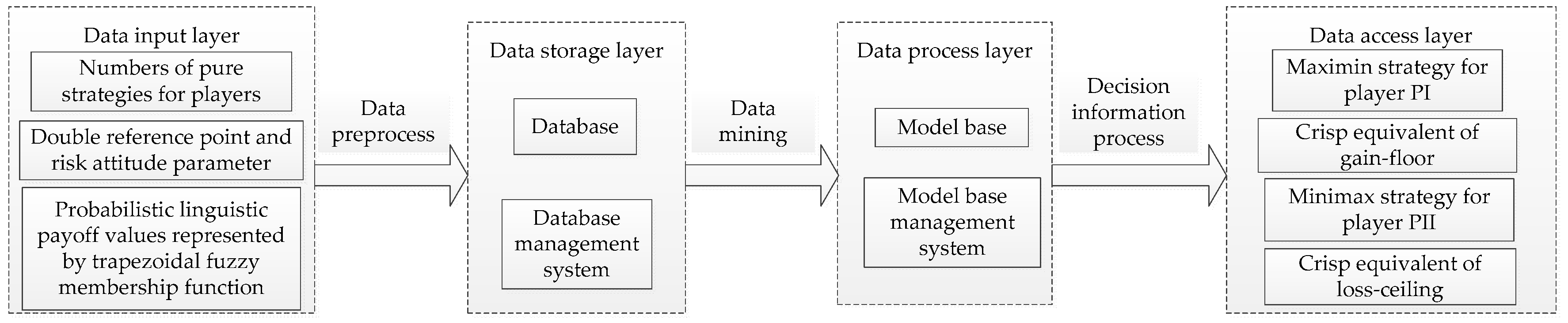
In order to show the practical value of the proposed method, a decision support system (DSS) is designed, which is based on the platform of Windows 11 by combining Microsoft SQL Server 2015 with Java. Figure 14 displays the framework of DSS based on the proposed method.

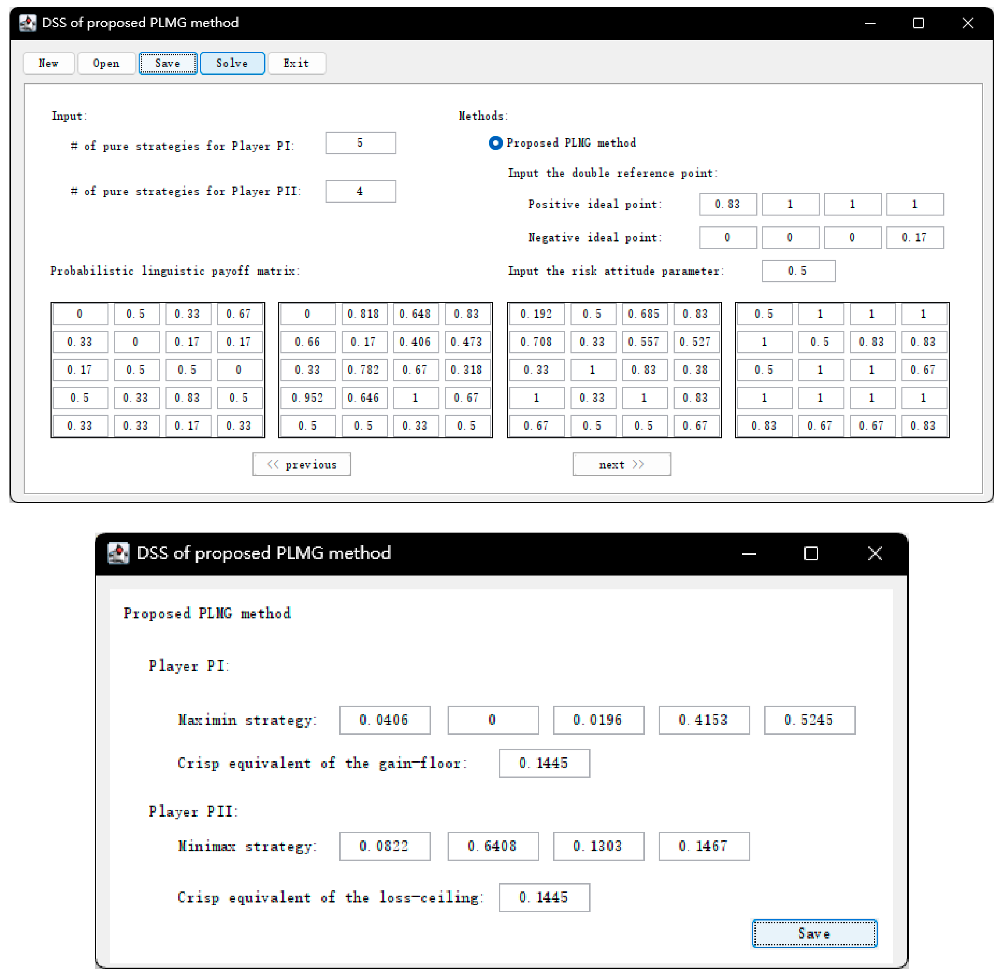
To further explain the practicality of the proposed method, the main interfaces are shown as the following Figure 15 when using the developed DSS to solve the development strategy of SNNR in Section 6.1. In real world decision-making, the DMs only input four matrices and other parameters, then run the DSS, which can output the decision results.

Remark 3.

According to the DSS designed above, the decision-maker can quickly obtain the optimal strategy only by inputting the numbers of pure strategies for players, the payoff values expressed by trapezoidal membership function, double reference points and the risk attitude parameter. Thus, the process of the proposed method can be simplified by using the DSS.

The proposed method not only narrows the theoretical gap of matrix games in the context of probabilistic linguistic, but also has important practical value. Different from other matrix game methods, the proposed method aims to realize the long-term harmonious development of man and Nature. In addition, it is more practical for decision makers to choose a mixed strategy rather than a single pure strategy. The limitation of this study is that the developed method fails to investigate the multi-objective problems under a probabilistic linguistic environment, which is a deserving and interesting topic for the future. Besides, how to integrate other theories (e.g., regret theory and evidential theory) into game theory to solve practical problems is another challenging research direction. Moreover, the evolutionary game with natural language information is also a fascinating research field.

References

1. Collins, B.C.; Kumral, M. Game theory for analyzing and improving environmental management in the mining industry. Resour. Policy 2020, 69, 101860. [Google Scholar] [CrossRef]
2. Dlouhy, M. Game theory, coalition formation and political power concentration in the Prague City Assembly. Polit. Ekon. 2016, 64, 747–761. [Google Scholar] [CrossRef] [Green Version]
3. Ma, J.H.; Wu, K.F. Complex system and influence of delayed decision on the stability of a triopoly price game model. Nonlinear. Dyn. 2013, 73, 1741–1751. [Google Scholar] [CrossRef]
4. Bigdeli, H.; Hassanpour, H.; Tayyebi, J. Multiobjective security game with fuzzy payoffs. Iran. J. Fuzzy Syst. 2019, 16, 89–101. [Google Scholar]
5. Mi, X.; Liao, H.; Zeng, X.; Xu, Z. The two-person and zero-sum matrix game with probabilistic linguistic information. Inf. Sci. 2021, 570, 487–499. [Google Scholar] [CrossRef]
6. Xue, W.; Xu, Z.; Mi, X. Solving hesitant fuzzy linguistic matrix game problems for multiple attribute decision making with prospect theory. Comput. Ind. Eng. 2021, 161, 107619. [Google Scholar] [CrossRef]
7. Li, D.F. Linear programming approach to solve interval-valued matrix games. Omega 2011, 39, 655–666. [Google Scholar] [CrossRef]
8. Li, D.F. A fast approach to compute fuzzy values of matrix games with payoffs of triangular fuzzy numbers. Eur. J. Oper. Res. 2012, 223, 421–429. [Google Scholar] [CrossRef]
9. Li, D.F. An effective methodology for solving matrix games with fuzzy payoffs. IEEE Trans. Cybern. 2013, 43, 610–621. [Google Scholar] [PubMed]
10. Yang, J.; Xu, Z.; Dai, Y. Simple noncooperative games with intuitionistic fuzzy information and application in ecological management. Appl. Intell. 2021, 51, 6685–6697. [Google Scholar] [CrossRef]
11. Li, D.F. Mathematical-programming approach to matrix games with payoffs represented by Atanassov’s interval-valued intuitionistic fuzzy sets. IEEE Trans. Fuzzy Syst. 2010, 18, 1112–1128. [Google Scholar] [CrossRef]
12. Jana, J.; Roy, S.K. Dual hesitant fuzzy matrix games: Based on new similarity measure. Soft Comput. 2019, 23, 8873–8886. [Google Scholar] [CrossRef]
13. Karmakar, S.; Seikh, M.R.; Castillo, O. Type-2 intuitionistic fuzzy matrix games based on a new distance measure: Application to biogas-plant implementation problem. Appl. Soft Comput. 2021, 106, 107357. [Google Scholar] [CrossRef]
14. Xue, W.; Xu, Z.; Zeng, X.J. Solving matrix games based on Ambika method with hesitant fuzzy information and its application in the counter-terrorism issue. Appl. Intell. 2021, 51, 1227–1243. [Google Scholar] [CrossRef]
15. Vijay, V.; Chandra, S.; Bector, C.R. Matrix games with fuzzy goals and fuzzy pay offs. Omega 2015, 33, 425–429. [Google Scholar] [CrossRef]
16. Li, D.F. Lexicographic method for matrix games with payoffs of triangular fuzzy numbers. Int. J. Uncertain. Fuzzy Knowl. Based Syst. 2018, 16, 371–389. [Google Scholar] [CrossRef]
17. Sahoo, L. Solving matrix games with linguistic payoffs. Int. J. Syst. Assur. Eng. 2019, 10, 484–490. [Google Scholar] [CrossRef]
18. Singh, A.; Gupta, A.; Mehra, A. Matrix games with 2-tuple linguistic information. Ann. Oper. Res. 2020, 287, 895–910. [Google Scholar] [CrossRef]
19. Verma, R.; Aggarwal, A. On matrix games with 2-tuple intuitionistic fuzzy linguistic payoffs. Iran. J. Fuzzy Syst. 2021, 18, 149–167. [Google Scholar]
20. Wang, H.; Xu, Z.; Zeng, X.J. Modeling complex linguistic expressions in qualitative decision making: An overview. Knowl. Based Syst. 2018, 144, 174–187. [Google Scholar] [CrossRef] [Green Version]
21. Rodríguez, R.M.; Martínez, L.; Herrera, F. Hesitant fuzzy linguistic term sets for decision making. IEEE Trans. Fuzzy Syst. 2012, 20, 109–119. [Google Scholar] [CrossRef]
22. Pang, Q.; Wang, H.; Xu, Z.S. Probabilistic linguistic term sets in multi-attribute group decision making. Inf. Sci. 2016, 369, 128–143. [Google Scholar] [CrossRef]
23. Lin, M.; Chen, Z.; Xu, Z.; Gou, X.; Herrera, F. Score function based on concentration degree for probabilistic linguistic term sets: An application to TOPSIS and VIKOR. Inf. Sci. 2021, 551, 270–290. [Google Scholar] [CrossRef]
24. You, X.; Hou, F. A self-confidence and leadership based feedback mechanism for consensus of group decision making with probabilistic linguistic preference relation. Inf. Sci. 2022, 582, 547–572. [Google Scholar] [CrossRef]
25. Xian, S.; Chai, J.; Yin, Y. A visual comparison method and similarity measure for probabilistic linguistic term sets and their applications in multi-criteria decision making. Int. J. Fuzzy Syst. 2019, 21, 1154–1169. [Google Scholar] [CrossRef]
26. Liu, P.; Teng, F. Probabilistic linguistic TODIM method for selecting products through online product reviews. Inf. Sci. 2019, 485, 441–455. [Google Scholar] [CrossRef]
27. Liu, P.; Li, Y. An extended MULTIMOORA method for probabilistic linguistic multi-criteria group decision-making based on prospect theory. Comput. Ind. Eng. 2019, 136, 528–545. [Google Scholar] [CrossRef]
28. Liao, H.; Jiang, L.; Lev, B.; Fujita, H. Novel operations of PLTSs based on the disparity degrees of linguistic terms and their use in designing the probabilistic linguistic ELECTRE III method. Appl. Soft Comput. 2019, 80, 450–464. [Google Scholar] [CrossRef]
29. Bhaumik, A.; Roy, S.K.; Weber, G.W. Multi-objective linguistic-neutrosophic matrix game and its applications to tourism management. J. Dyn. Games 2021, 8, 101–118. [Google Scholar] [CrossRef]
30. Kahneman, D.; Tversky, A. Prospect theory: An analysis of decision under risk. Econometrica 1979, 47, 263–291. [Google Scholar] [CrossRef] [Green Version]
31. Wu, A.; Li, H.; Dong, M. A novel two-stage method for matching the technology suppliers and demanders based on prospect theory and evidence theory under intuitionistic fuzzy environment. Appl. Soft Comput. 2020, 95, 106553. [Google Scholar] [CrossRef]
32. Zhou, X.; Wang, L.; Liao, H.; Wang, S.; Lev, B.; Fujita, H. A prospect theory-based group decision approach considering consensus for portfolio selection with hesitant fuzzy information. Knowl. Based Syst. 2019, 168, 28–38. [Google Scholar] [CrossRef]
33. Xu, H.; Liu, P.; Teng, F. Two prospect theory-based decision-making models using data envelopment analysis with hesitant fuzzy linguistic information. Inf. Sci. 2022, 582, 415–438. [Google Scholar] [CrossRef]
34. Wan, S.P.; Zou, W.C.; Dong, J.Y.; Martínez, L. A probabilistic linguistic dominance score method considering individual semantics and psychological behavior of decision makers. Expert Syst. Appl. 2021, 184, 115372. [Google Scholar] [CrossRef]
35. Metzger, L.P.; Rieger, M.O. Non-cooperative games with prospect theory players and dominated strategies. Game. Econ. Behav. 2019, 115, 396–409. [Google Scholar] [CrossRef]
36. Shen, J.; Gao, X.; He, W.; Sun, F.; Zhang, Z.; Kong, Y.; Wan, Z.; Zhang, X.; Zhang, L.; Wang, J.; et al. Prospect theory in an evolutionary game: Construction of watershed ecological compensation system in Taihu Lake Basin. J. Clean. Prod. 2021, 291, 125929. [Google Scholar] [CrossRef]
37. Wan, S.P.; Chen, Z.H.; Dong, J.Y. Bi-objective trapezoidal fuzzy mixed integer linear program-based distribution center location decision for large-scale emergencies. Appl. Soft Comput. 2021, 110, 107757. [Google Scholar] [CrossRef]
38. Yager, R.R. On ordered weighted averaging aggregation operators in multicriteria decision making. IEEE Trans. Syst. Man Cybern. 1988, 18, 183–190. [Google Scholar] [CrossRef]
39. Filev, D.; Yager, R. On the issue of obtaining OWA operator weights. Fuzzy Sets Syst. 1998, 94, 157–169. [Google Scholar] [CrossRef]
40. Tversky, A.; Kahneman, D. Advances in prospect theory: Cumulative representation of uncertainty. J. Risk Uncertain. 1992, 5, 297–323. [Google Scholar] [CrossRef]
41. Li, D.F.; Hong, F.X. Solving constrained matrix games with payoffs of triangular fuzzy numbers. Comput. Math. Appl. 2012, 64, 432–446. [Google Scholar] [CrossRef] [Green Version]
42. Merigo, J.M.; Wei, G.W. Probabilistic aggregation operators and their application in uncertain multi-person decision making. Technol. Econ. Dev. Econ. 2011, 17, 335–351. [Google Scholar] [CrossRef]
43. Liu, H.; Rodríguez, R.M. A fuzzy envelope for hesitant fuzzy linguistic term set and its application to multicriteria decision making. Inf. Sci. 2014, 258, 220–238. [Google Scholar] [CrossRef]
44. Liao, H.C.; Xu, Z.S. Approaches to manage hesitant fuzzy linguistic information based on the cosine distance and similarity measures for HFLTSs and their application in qualitative decision making. Expert Syst. Appl. 2015, 42, 5328–5336. [Google Scholar] [CrossRef]
45. Zhao, X.; Wang, J.; Ye, H.; Muhammad, A.; Wang, S. The Bowen ratio of an alpine grassland in Three-River Headwaters, Qinghai-Tibet Plateau, from 2001 to 2018. J. Resour. Ecol. 2021, 12, 305–318. [Google Scholar]
46. Chu, H.; Wei, J.; Qiu, J.; Li, Q.; Wang, G. Identification of the impact of climate change and human activities on rainfall-runoff relationship variation in the Three-River Headwaters region. Ecol. Indic. 2019, 106, 105516. [Google Scholar] [CrossRef]
47. Bai, Y.; Guo, C.; Degen, A.A.; Ahmad, A.A.; Wang, W.; Zhang, T.; Li, W.; Ma, L.; Huang, M.; Zeng, H.; et al. Climate warming benefits alpine vegetation growth in Three-River Headwater Region, China. Sci. Total Environ. 2020, 742, 140574. [Google Scholar] [CrossRef]
48. Zhang, X.; Jin, X. Vegetation dynamics and responses to climate change and anthropogenic activities in the Three-River Headwaters Region, China. Ecol. Indic. 2021, 131, 108223. [Google Scholar] [CrossRef]
49. Liu, D.; Cao, C.; Dubovyk, O.; Tian, R.; Chen, W.; Zhuang, Q.; Zhao, Y.; Menz, G. Using fuzzy analytic hierarchy process for spatio-temporal analysis of eco-environmental vulnerability change during 1990–2010 in Sanjiangyuan region, China. Ecol. Indic. 2017, 73, 612–625. [Google Scholar] [CrossRef]
50. Zeng, Y.; Zhong, L.; Wang, L. Spatiotemporal changes in recreation potential of ecosystem services in Sanjiangyuan China. J. Spat. Sci. 2018, 63, 359–377. [Google Scholar]
Figure 1. Flowchart of the proposed method.
Mathematics 10 01070 g001
Figure 2. Linguistic terms and corresponding triangular fuzzy membership functions.
Mathematics 10 01070 g002
Figure 3. Fuzzy envelopes obtained from Example 2.
Mathematics 10 01070 g003
Figure 4. Framework of the proposed method.
Mathematics 10 01070 g004
Figure 5. y i with parameter η varying from 0 to 1.
Mathematics 10 01070 g005
Figure 6. z j with parameter η varying from 0 to 1.
Mathematics 10 01070 g006
Figure 7. Gain-floor U and loss-ceiling V with parameter η varying from 0 to 1.
Mathematics 10 01070 g007
Figure 8. y i with parameter η varying from 0 to 1.
Mathematics 10 01070 g008
Figure 9. z j with parameter η varying from 0 to 1.
Mathematics 10 01070 g009
Figure 10. Gain-floors U and U 2 with parameter η varying from 0 to 1.
Mathematics 10 01070 g010
Figure 11. y i with parameter η varying from 0 to 1.
Mathematics 10 01070 g011
Figure 12. z j with parameter η varying from 0 to 1.
Mathematics 10 01070 g012
Figure 13. The gain-floor U and U 3 with parameter η varying from 0 to 1.
Mathematics 10 01070 g013
Figure 14. Framework of DSS based on the proposed method.
Mathematics 10 01070 g014
Figure 15. Main interfaces of results obtained by the proposed method.
Mathematics 10 01070 g015