Complexity of Solutions Combination for the Three-Index Axial Assignment Problem

Abstract

In this work we consider the NP-hard three-index axial assignment problem. We formulate and investigate a problem of combining feasible solutions. Such combination can be applied in a wide range of heuristic and approximate algorithms for solving the assignment problem, instead of the commonly used strategy of selecting the best solution among the found feasible solutions. We discuss approaches to a solution of the combination problem and prove that it becomes NP-hard already in the case of combining four solutions.

1. Introduction

Multi-index axial assignment problems arise when it comes to solving a multitude of applied problems in the logistics and planning area [1,2,3]. An overview of the results obtained through analysis of the subclasses of multi-index assignment problems is given in [1]. The class of multi-index axial assignment problems is known to be NP-hard even in the three-index case [4]. In [5] it was proved that no polynomial ε-approximate algorithms for solving a three-index axial assignment problem (here ε is an arbitrary constant) exist, otherwise P = NP.

There are known approximate and heuristic algorithms for solving the NP-hard axial assignment problem [2,6,7,8,9,10,11]. As a rule, such algorithms construct a series of feasible solutions to the problem. The general approach in the final step of the algorithms is choosing the best solution from the constructed feasible solutions. As an improvement of the final step of such algorithms we propose building an optimal combination of the found feasible solutions instead of commonly applied selection of the best solution. The optimal combination of feasible solutions is an optimization problem where the fragments of the found feasible solutions need to be optimally combined. Obviously, such an optimal combination is no worse than a standard selection of the best solution. But, as we will demonstrate later, solutions combination outperforms (based on computational experiments) selection of the best solution while having comparable computational complexity.

The solutions combination problem was first formulated in our earlier paper [12]. In this work a linear complexity algorithm for optimal combining of a pair of feasible solutions was constructed. Heuristic algorithms for combining of three and a larger number of solutions were proposed in [13]. These heuristics are based on successive combination of pairs of solutions. An efficient algorithm for optimal combining of three and larger number of solutions was an open problem.

In this work we have proved that the solution combination problem is already NP-hard in the case of combining four solutions. Which means that there is already no polynomial algorithm for optimal combination in the case of four solutions, otherwise $P=NP.$ An efficient algorithm for optimal combining in the case of three solutions remains an open problem.

Further the article is organized as follows. In Section 2 we formulate the axial assignment problem and the corresponding solutions combination problem. Section 3 deals with the results of designing the algorithms for combining feasible solutions. Finally, in Section 4 the NP-hardness of combining four solutions is proved.

2. Solutions Combination Problem

Let $I,J,K$ be the disjoint index sets, $I\cap J=\varnothing , I\cap K=\varnothing , J\cap K=\varnothing \mathrm{and} \left|I\right|=\left|J\right|=\left|K\right|=n$; $c_{ijk}, i\in I,j\in J,k\in K$ is the three-index cost matrix; and $x_{ijk},i\in I,j\in J,k\in K$ is the three-index matrix of the variables. Then the three-index axial assignment problem is formulated as the following integer linear programming problem:

$${\displaystyle \sum }_{i\in I}{\displaystyle \sum }_{j\in J}{x}_{ijk}=1,k\in K,$$

(1)

$${\displaystyle \sum }_{i\in I}{\displaystyle \sum }_{k\in K}{x}_{ijk}=1, j\in J,$$

(2)

$${\displaystyle \sum }_{j\in J}{\displaystyle \sum }_{k\in K}{x}_{ijk}=1, i\in I,$$

(3)

$$x_{ijk}\in \left\{0,1\right\},i\in I,j\in J,k\in K,$$

(4)

$${\displaystyle \sum }_{i\in I}{\displaystyle \sum }_{j\in J}{\displaystyle \sum }_{k\in K}{c}_{ijk}{x}_{ijk}\to \min .$$

(5)

Next, let a set $W\subseteq I\times J\times K$ be given that defines a subset of the allowed assignments:

$$x_{ijk}=0,\left(i,j,k\right)\notin W.$$

(6)

Then we consider an optimization problem with objective (5) subject to constraints (1)–(4) and denote it by $Z\left(W\right)$ for the given subset $W$. It is obvious that problem (1)–(5) corresponds to the problem $Z\left(I\times J\times K\right)$.

In the general case problem $Z\left(W\right)$ is NP-hard [1]. Moreover, the problem of feasibility check of system (1)–(4), (6) for an arbitrary set $W$ is NP-complete [1]. We will further consider subsets $W$ such that correspond to the assignments set of some feasible solutions of the problem (1)–(5).

We introduce auxiliary notations. Let $x$ be a feasible solution to the system of constraints (1)–(4). Then $W\left(x\right)$ will be used to denote the following set of allowed assignments:

$$W\left(x\right)=\left\{\left(i,j,k\right)\right|x_{ijk}^{}=1,i\in I,j\in J,k\in K\}.$$

Let $x^1$,$x^2,\dots ,x_{}^m$ be some arbitrary feasible solutions of the system (1)–(4). Denote $W\left(x^1,x^2, \dots ,x^m\right)={{\displaystyle \mathrm{U}}}_{t=1}^{m}W\left(x^t\right)$. Then the problem of optimal combining of $m$ feasible solutions $x^1$,$x^2,\dots ,x_{}^m$ takes the form $Z\left(W\left(x^1,x^2, \dots ,x^m\right)\right)$.

A large number of known heuristic and approximate algorithms for solving the axial assignment problem yield, in the course of their operation, a certain set of feasible solutions (for convenience denoted by $x^1$,$x^2,\dots ,x_{}^m$). Denote $C\left(x\right)={\displaystyle \sum }_{i\in I}{\displaystyle \sum }_{j\in J}{\displaystyle \sum }_{k\in K}{c}_{ijk}{x}_{ijk}.$ The general approach in the final step of these algorithms is choosing the best solution from the constructed feasible solutions, i.e., $C^{\prime }={\min }_{t=\overline{1,m}}C\left(x^t\right)$. As an improvement on the final step of such algorithms, i.e., selection of the best solution, we propose building an optimal combination of the found feasible solutions through solving the problem $Z\left(W\left(x^1,x^2, \dots ,x^m\right)\right)$. In other words, we propose building a solution by combining the components of the found feasible solutions rather than only choosing the best one.

3. Solution Combination Algorithms

Let us consider algorithms for solutions combination problem $Z\left(W\left(x^1,x^2, \dots ,x^m\right)\right)$. In our earlier paper [12] we constructed a linear complexity algorithm for solutions combination problem for the case m = 2.

It was proved in [12] that Algorithm 1 finds solution of the problem $Z\left(W\left(x^1,x^2\right)\right)$ and requires O(n) computational operations. Thus, in accordance with step 5 of Algorithm 1, the optimal value of the criterion for problem $Z\left(W\left(x^1,x^2\right)\right)$ is defined as ${\displaystyle \sum }_{l=1}^q\min \left({\displaystyle \sum }_{\left(i,j,k\right)\in D_l^1}{c}_{ijk},{\displaystyle \sum }_{\left(i,j,k\right)\in D_l^2}{c}_{ijk}\right)$.

Algorithm 1. Ref. [12]. Solution of problem $Z\left(W\left(x^1,x^2\right)\right)$

Step 1. Construct graph $G=\left(V,A\right)$, where $V=\left\{I\cup J\cup K\right\}, A=\left\{\left(i,j\right),\left(i,k\right),\left(j,k\right)|\left(i,j,k\right)\in W\left(x^1,x^2\right)\right\}$.   Step 2. Find the connectivity components $V_l,l=\overline{1,q}$, of graph $G$ and build subgraphs $G_l=\left(V_l,A_l\right),l=\overline{1,q}$, induced by the corresponding components of connectivity.   Step 3. Now, we build the following sets:         $D_l^1=\left\{\left(i,j,k\right)|\left(i,j,k\right)\in W\left(x^1\right), \left(i,j\right),\left(i,k\right),\left(j,k\right)\in A_l\right\},$   $D_l^2=\left\{\left(i,j,k\right)|\left(i,j,k\right)\in W\left(x^2\right), \left(i,j\right),\left(i,k\right),\left(j,k\right)\in A_l\right\}$.   Step 4. The optimal value of criterion of the problem $Z\left(W\left(x^1,x^2\right)\right)$ is defined as   $c^{*}={\displaystyle \sum }_{l=1}^q\min \left({\displaystyle \sum }_{\left(i,j,k\right)\in D_l^1}{c}_{ijk},{\displaystyle \sum }_{\left(i,j,k\right)\in D_l^2}{c}_{ijk}\right)$.   Step 5. The optimal solution to the problem $Z\left(W\left(x^1,x^2\right)\right)$ is constructed as follows. Initially let $x_{ijk}≔0,i\in I,j\in J,k\in K$. Further, for each $l=\overline{1,q}$ perform         $x_{ijk}≔1, \left(i,j,k\right)\in D_l^{p^{*}}$, where $p^{*}=\underset{p\in \left\{1,2\right\}}{\mathrm{argmin}}{\displaystyle \sum }_{\left(i,j,k\right)\in D_l^p}{c}_{ijk}$.

We have demonstrated in [13] that an algorithm based on successive optimal combination of feasible solutions pairs does not ensure an optimal solution for the problem $Z\left(W\left(x^1,x^2, \dots ,x^m\right)\right)$ when $m=3$. However, such a successive combination technique can be used as a heuristic algorithm for the problem $Z\left(W\left(x^1,x^2, \dots ,x^m\right)\right)$ when $m\ge 3$. We provide the results of the computation experiments for a variety of successive combination strategies, which demonstrate the advantage of the proposed approach over the commonly used step of choosing the best feasible solution [13].

In [12,13] we presented comprehensive computational experiments for solutions combination algorithm for m = 2 and for solutions combination strategies for $m\ge$ 3. Below we will giving a brief description of these computational results. In [5] an approximate algorithm was constructed for the axial assignment problems satisfying triangle inequality. This approximate algorithm constructs three feasible solutions and chooses the best among them. A collection of test problems for $n\in \left\{33,66\right\}$ with the cost matrices satisfying triangle inequality was proposed in [5]. For the collection of the problems presented in [5] the solution combination algorithm gives 0.148% improvement compared to the original step of choosing the best solution by the approximate algorithm; for more details please see [12]. For a set of cost matrices whose entries were generated with integer values uniformly distributed at the interval $\left[0,300\right]$ and for $n\in \left\{10,11,\dots ,19\right\}$ we randomly generated $n^3$ feasible solutions and applied the local optimization algorithm proposed in [6]. Based on computational results we demonstrated that applying of successive combination strategies to the locally optimized solution gives approximately 4–8% improvement compared to a standard approach of choosing the best solution; for more details please see [13].

4. Solutions Combination NP-Hardness

We will now show that the class of problems of the optimal combination of m feasible solutions is NP-hard even when $m=4$. The proof is based on polynomial reduction of the well-known NP-hard class of 3-CNF problems [4]. Here 3-CNF is the problem of determining if a Boolean formula is satisfiable, where the Boolean formula is in conjunctive normal form with three variables per conjunct.

Theorem 1.

The class of 3-CNF problems is polynomially reduced to the class of 3-CNF problems without repeating variables in each clause.

Proof of Theorem 1.

Let us consider an arbitrary 3-CNF and apply the following algorithm to each clause of 3-CNF:

• If a clause does not contain any repeating variables, it remains unchanged.
• If a repeating variable is included into a clause only with or only without negation then a clause has the form $\left(x\cup x\cup y\right)$ or $\left(x\cup x\cup x\right)$, where $x, y$ are the literals. A clause $u\left(x,y\right)=\left(x\cup x\cup y\right)$ is replaced by $u^{\prime }\left(x,y,z\right)=\left(x\cup y\cup z\right)\cap \left(x\cup y\cup \overline{z}\right)$, where $z$ is the new Boolean variable. It is obvious that $u\left(x,y\right)=$ $u^{\prime }\left(x,y,z\right)$, $\forall z$. A clause $u\left(x\right)=\left(x\cup x\cup x\right)$ is replaced by $u^{\prime }\left(x,z,w\right)=\left(x\cup z\cup w\right)\cap \left(x\cup z\cup \overline{w}\right)\cap \left(x\cup \overline{z}\cup w\right)\cap \left(x\cup \overline{z}\cup \overline{w}\right),$ where $z,w$ are the new Boolean variables. It is obvious that $u\left(x\right)=$ $u^{\prime }\left(x,z,w\right)$, $\forall z,w$.
• If a repeating variable is included into a clause simultaneously with and without negation, this clause has the form $\left(x\cup \overline{x}\cup y\right)$, where $x$ is the Boolean variable, $y$ is the literal. Then $\left(x\cup \overline{x}\cup y\right)\equiv 1$, and the clause can be discarded from 3-CNF.

At this point we polynomially reduced the class of 3-CNF problems to the class of 3-CNF problems without repeating variables in each clause. The lemma is proved. □

Theorem 2.

The class of optimal combination of four solutions problems is NP-hard.

Proof of Theorem 2.

To prove the theorem, we will show that NP-hard class of 3-CNF problems [4] can be polynomially reduced to a class of optimal combination of four feasible solutions problems. □

Consider an arbitrary 3-CNF problem with $N$ Boolean variables and $M$ clauses. Let $L$ = $\left\{1,\dots ,N\right\}$ be the set of indices of Boolean variables of the 3-CNF. According to theorem 1, without loss of generality we assume that there are no repeating variables in each clause. For convenience, we introduce the following notations:

• $l_1\left(s\right),l_2\left(s\right),l_3\left(s\right)$ are the indices of Boolean variables in the $s$-th clause;
• $L\left(s\right)=\left\{l_1\left(s\right)\cup l_2\left(s\right)\cup l_3\left(s\right)\right\}$ is the set of indices of the Boolean variables included into the s-th clause;
• $L^{+}\left(s\right)\subseteq L\left(s\right)$ is the set of indices of the Boolean variables included without negation into the s-th clause;
• $L^{-}\left(s\right)\subseteq L\left(s\right)$ is the set of indices of the Boolean variables included with negation into the s-th clause;
• $\overline{L}\left(s\right)=\left\{1,\dots ,N\right\}\backslash L\left(s\right)$ is the set of indices for the Boolean variables that are not included into the $s$-th clause,

$$s=\overline{1,M}.$$

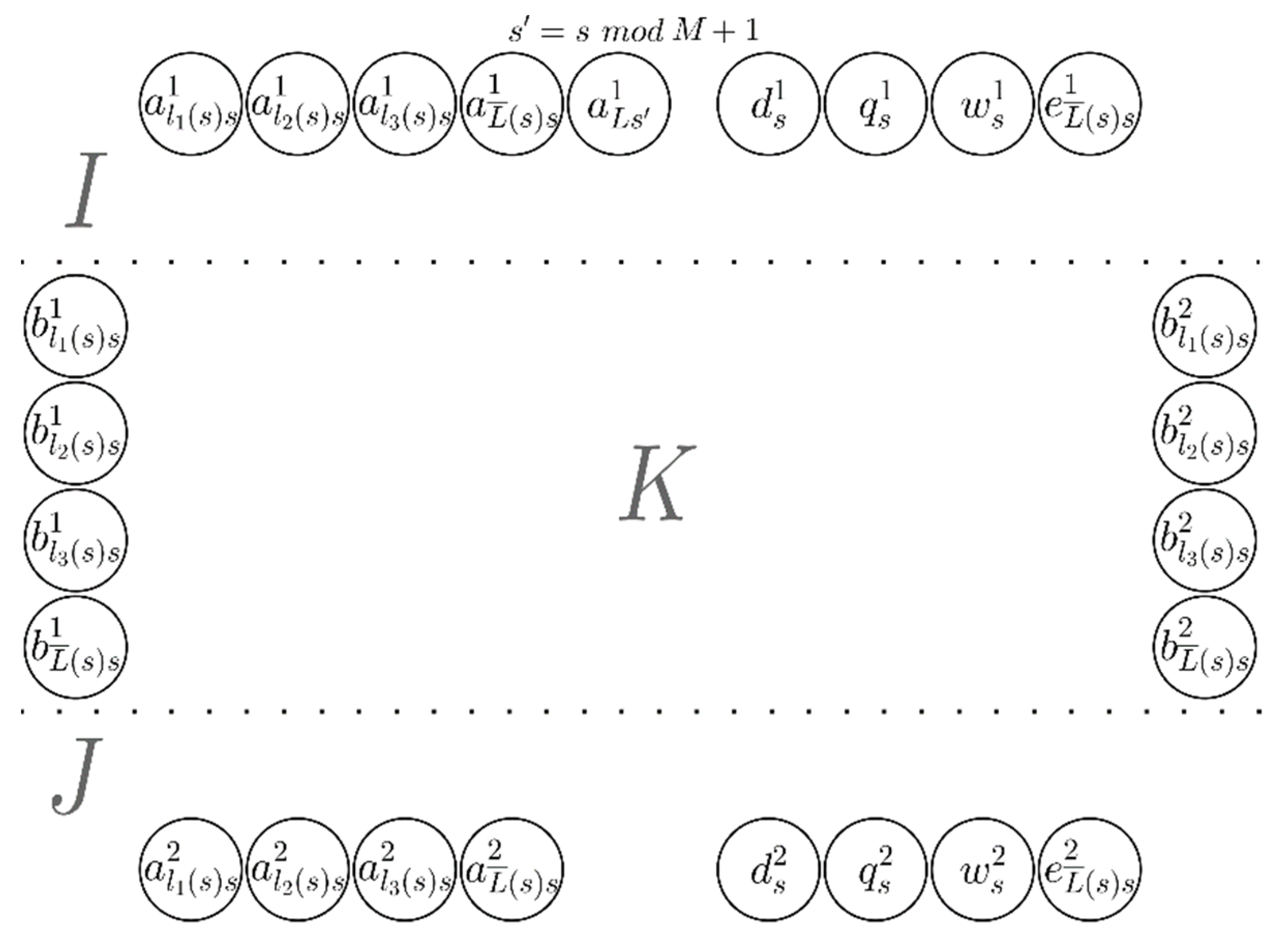
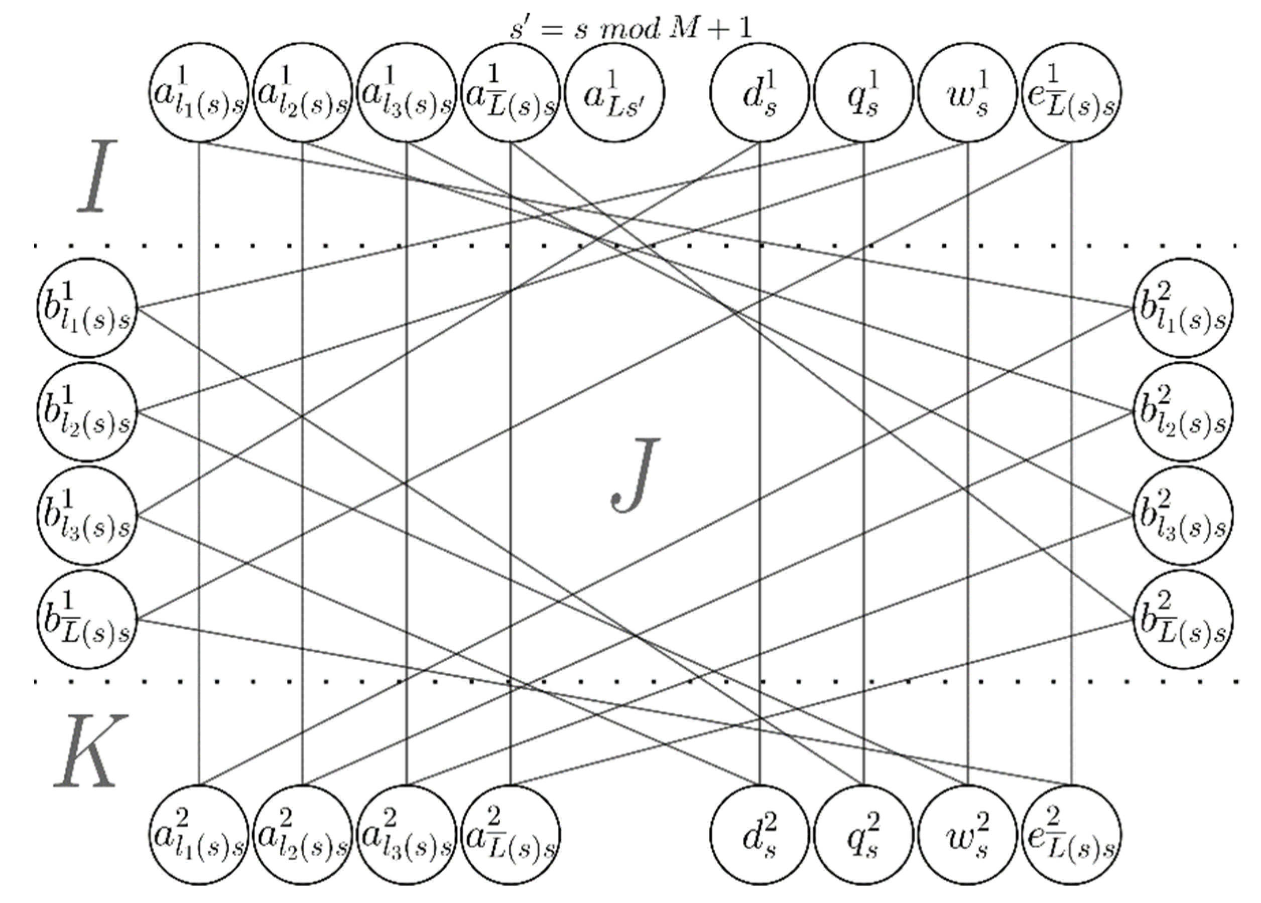
Then we construct disjoint sets of indices $I,J,K$ as follows; see Figure 1 for visualization of these sets:

• $I=\left\{a_{ls}^1|l=\overline{1,N},s=\overline{1,M}\right\}\cup \left\{d_s^1,q_s^1,w_s^1|s=\overline{1,M}\right\}\cup \left\{e_{ls}^1\right|l\in \overline{L}\left(s\right),s=\overline{1,M}\}$,
• $J=\left\{a_{ls}^2|l=\overline{1,N},s=\overline{1,M}\right\}\cup \left\{d_s^2,q_s^2,w_s^2|s=\overline{1,M}\right\}\cup \left\{e_{ls}^2\right|l\in \overline{L}\left(s\right),s=\overline{1,M}\}$,
• $K=\left\{b_{ls}^1,b_{ls}^2|l=\overline{1,N},s=\overline{1,M}\right\}$.

According to above construction, $\left|I\right|=\left|J\right|=NM+3M+\left(N-3\right)M=2NM$, $\left|K\right|=2NM$. Hence, $\left|I\right|=\left|J\right|=\left|K\right|=2NM$.

Next, build a set $R\subseteq I\times J\times K$ to be used for defining a multi-index cost matrix of the axial assignment problem in the following form:

• $R_1=\{(a_{ls}^1,a_{ls}^2,b_{ls}^1),(a_{l\left(s \mathrm{mod} M+1\right)}^1,a_{ls }^2,b_{ls}^2)|l=\overline{1,N},s=\overline{1,M}\}$;
• $R_2=\{(d_s^1,d_s^2,b_{ls}^1\left)\right|l\in L^{-}\left(s\right),s=\overline{1,M}\}\cup \{(d_s^1,d_s^2,b_{ls}^2\left)\right|l\in L^{+}\left(s\right),s=\overline{1,M}\}$;
• $R_3=\{\left(q_s^1,q_s^2,b_{l_1\left(s\right)s}^1\right),\left(q_s^1,q_s^2,b_{l_1\left(s\right)s}^2\right),\left(q_s^1,q_s^2,b_{l_2\left(s\right)s}^1\right),\left(q_s^1,q_s^2,b_{l_2\left(s\right)s}^2\right)|s=\overline{1,M}\}$;
• $R_4=\{\left(w_s^1,w_s^2,b_{l_2\left(s\right)s}^1\right),\left(w_s^1,w_s^2,b_{l_2\left(s\right)s}^2\right),\left(w_s^1,w_s^2,b_{l_3\left(s\right)s}^1\right),\left(w_s^1,w_s^2,b_{l_3\left(s\right)s}^2\right)|s=\overline{1,M}\}$;
• $R_5=\{(e_{ls}^1,e_{ls}^2,b_{ls}^1),(e_{ls}^1,e_{ls}^2,b_{ls}^2)|l\in \overline{L}\left(s\right),s=\overline{1,M}\}$;
• $R=R_1\cup R_2\cup R_3\cup R_4\cup R_5$.

Now we can define the three-index cost matrix as

$$c_{ijk}=\{\begin{array}{l}0, \left(i,j,k\right)\in R\\ 1, \mathrm{otherwise}\end{array}, i\in I,j\in J,k\in K.$$

The constructed sets $I,J,K$ and three-index cost matrix $\Vert c_{ijk}\Vert$ define the three-index axial assignment problem (1)–(5).

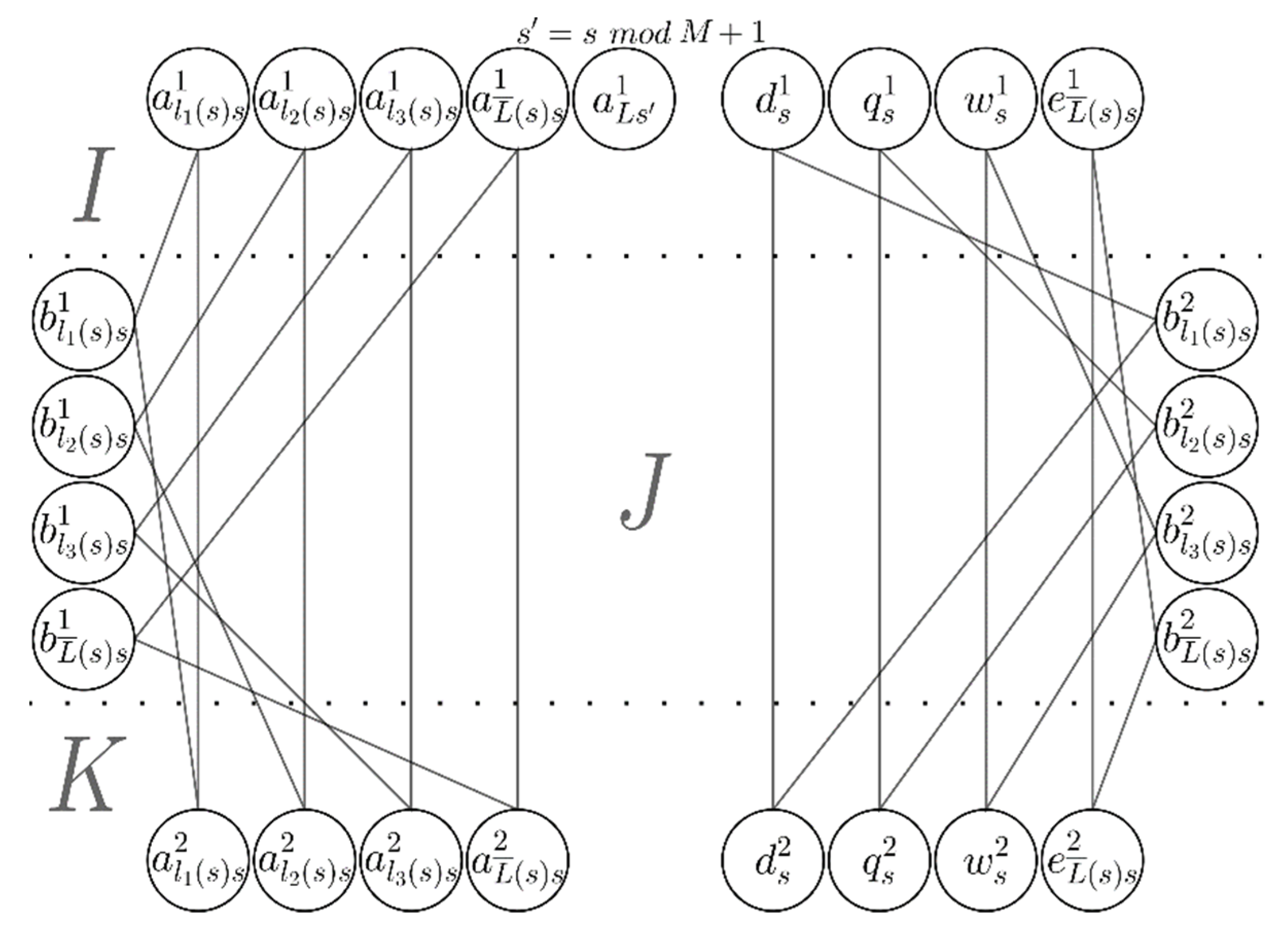
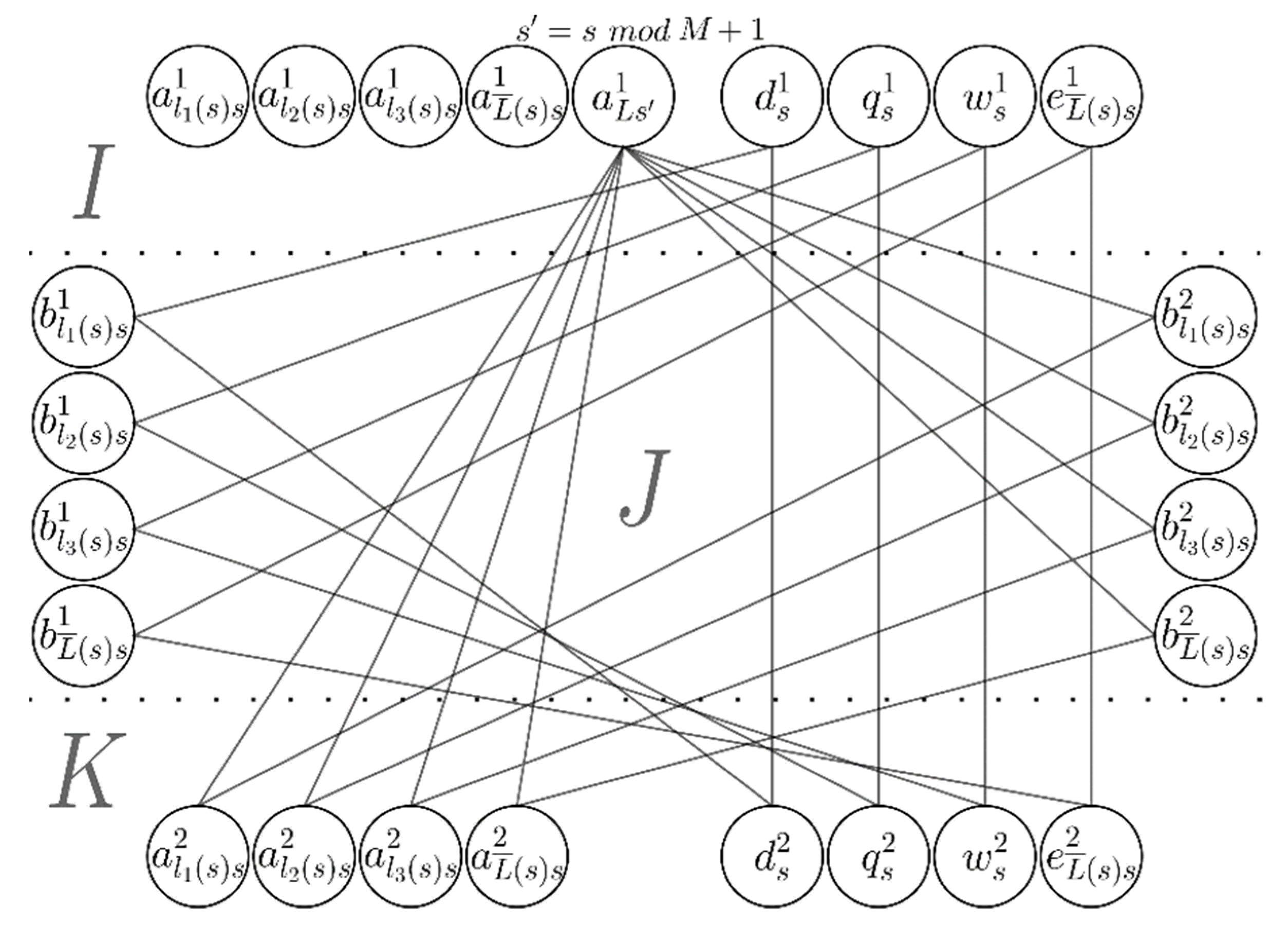
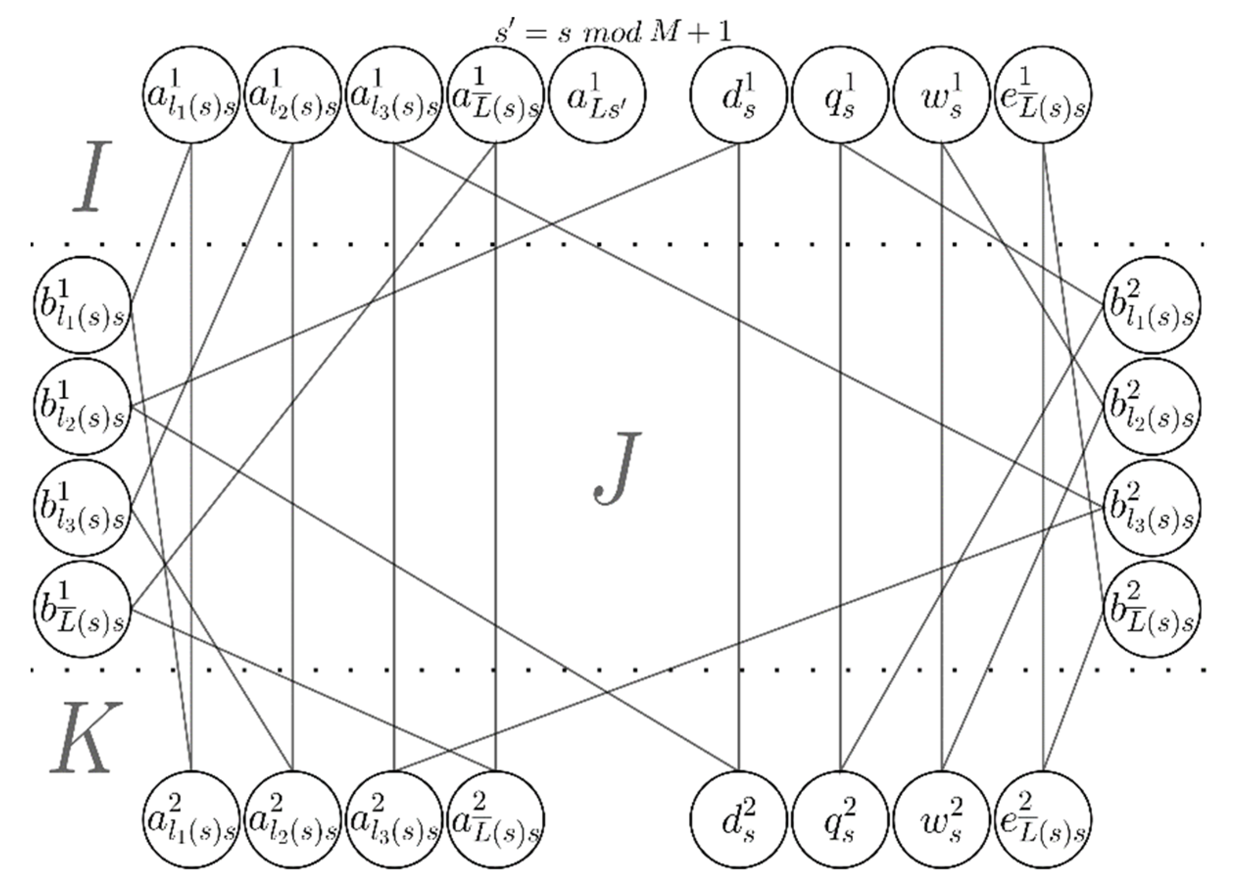
Further we build four subsets $P_1,P_2,P_3,P_4\subseteq$ $I\times J\times K$, that will determine four feasible solutions to problem (1)–(5); see Figure 2, Figure 3, Figure 4 and Figure 5 for visualization of the sets $P_1$–$P_4$.:

• $\begin{array}{l}{P}_1=\{(a_{ls}^1,a_{ls}^2,b_{ls}^1\left)\right|l=\overline{1,N},s=\overline{1,M}\}\cup \{(q_s^1,q_{s }^2,b_{l_2\left(s\right)s}^2),(w_s^1,w_{s }^2,b_{l_3\left(s\right)s}^2)|s=\overline{1,M}\}\cup \\ \{(d_s^1,d_{s }^2,b_{l_1\left(s\right)s}^2)|s=\overline{1,M}\}\cup \{\left(e_{ls}^1,e_{ls}^2,b_{ls}^2\right)|l\in \overline{L}\left(s\right),s=\overline{1,M}\}\end{array}$;
• $\begin{array}{l}{P}_2=\{(a_{l\left(s \mathrm{mod} M+1\right)}^1,a_{ls}^2,b_{ls}^2\left)\right|l=\overline{1,N},s=\overline{1,M}\}\cup \{(q_s^1,q_{s }^2,b_{l_2\left(s\right)s}^1),(w_s^1,w_{s }^2,b_{l_3\left(s\right)s}^1)|s=\overline{1,M}\}\\ \cup \{(d_s^1,d_{s }^2,b_{l_1\left(s\right)s}^1)|s=\overline{1,M}\}\cup \{\left(e_{ls}^1,e_{ls}^2,b_{ls}^1\right)|l\in \overline{L}\left(s\right),s=\overline{1,M}\}\end{array}$;
• $\begin{array}{l}{P}_3=\{(q_s^1,q_s^2,b_{l_1\left(s\right)s}^2),(w_s^1,w_s^2,b_{l_2\left(s\right)s}^2),\left(a_{l_1\left(s\right)s}^1,a_{l_1\left(s\right)s}^2,b_{l_1\left(s\right)s}^1\right)|s=\overline{1,M}\}\cup \\ \{(d_s^1,d_{s }^2,b_{l_2\left(s\right)s}^1),\left(a_{l_2\left(s\right)s}^1,a_{l_2\left(s\right)s}^2,b_{l_3\left(s\right)s}^1\right),\left(a_{l_3\left(s\right)s}^1,a_{l_3\left(s\right)s}^2,b_{l_3\left(s\right)s}^2\right)|l_2\left(s\right)\in L^{-}\left(s\right),s=\overline{1,M}\}\cup \\ \{(d_s^1,d_{s }^2,b_{l_3\left(s\right)s}^1),\left(a_{l_3\left(s\right)s}^1,a_{l_3\left(s\right)s}^2,b_{l_3\left(s\right)s}^2\right)|l_2\left(s\right)\in L^{+}\left(s\right),l_3\left(s\right)\in L^{-}\left(s\right),s=\overline{1,M}\}\cup \\ \{(d_s^1,d_{s }^2,b_{l_3\left(s\right)s}^2),\left(a_{l_3\left(s\right)s}^1,a_{l_3\left(s\right)s}^2,b_{l_3\left(s\right)s}^1\right)|l_2\left(s\right)\in L^{+}\left(s\right),l_3\left(s\right)\in L^{+}\left(s\right),s=\overline{1,M}\}\cup \\ \left\{(a_{l_2\left(s\right)s}^1,a_{l_2\left(s\right)s}^2,b_{l_2\left(s\right)s}^1)\right|l_2\left(s\right)\in L^{+}\left(s\right),s=\overline{1,M}\}\cup \\ \left\{\left(a_{ls}^1,a_{ls}^2,b_{ls}^1\right),\left(e_{ls}^1,e_{ls}^2,b_{ls}^2\right)|l\in \overline{L}\left(s\right),s=\overline{1,M}\right\}\end{array}$;
• $\begin{array}{l}{P}_4=\{(q_s^1,q_s^2,b_{l_1\left(s\right)s}^1),(w_s^1,w_s^2,b_{l_2\left(s\right)s}^1),\left(a_{l_1\left(s\right)s}^1,a_{l_1\left(s\right)s}^2,b_{l_1\left(s\right)s}^2\right)|s=\overline{1,M}\}\cup \\ \{(d_s^1,d_{s }^2,b_{l_2\left(s\right)s}^2),\left(a_{l_3\left(s\right)s}^1,a_{l_3\left(s\right)s}^2,b_{l_3\left(s\right)s}^1\right),\left(a_{l_2\left(s\right)s}^1,a_{l_2\left(s\right)s}^2,b_{l_3\left(s\right)s}^2\right)|l_2\left(s\right)\in L^{+}\left(s\right),s=\overline{1,M}\}\cup \end{array}$
  $\begin{array}{l}\{(d_s^1,d_{s }^2,b_{l_3\left(s\right)s}^1),\left(a_{l_3\left(s\right)s}^1,a_{l_3\left(s\right)s}^2,b_{l_3\left(s\right)s}^2\right)|l_2\left(s\right)\in L^{-}\left(s\right),l_3\left(s\right)\in L^{-}\left(s\right),s=\overline{1,M}\}\cup \\ \{(d_s^1,d_{s }^2,b_{l_3\left(s\right)s}^2),\left(a_{l_3\left(s\right)s}^1,a_{l_3\left(s\right)s}^2,b_{l_3\left(s\right)s}^1\right)|l_2\left(s\right)\in L^{-}\left(s\right),l_3\left(s\right)\in L^{+}\left(s\right),s=\overline{1,M}\}\cup \\ \left\{\left(a_{l_2\left(s\right)s}^1,a_{l_2\left(s\right)s}^2,b_{l_2\left(s\right)s}^2\right)\right|l_2\left(s\right)\in L^{-}\left(s\right),s=\overline{1,M}\}\cup \{\left(a_{ls}^1,a_{ls}^2,b_{ls}^2\right),\left(e_{ls}^1,e_{ls}^2,b_{ls}^1\right)|l\in \overline{L}\left(s\right),\\ s=\overline{1,M}\}\end{array}$.

The corresponding four feasible solutions $x^1,$ $x^2,$ $x^3,$ $x^4$ will be defined as follows:

$$x_{ijk}^t=\{\begin{array}{l}1, \mathrm{if} \left(i,j,k\right)\in P_t\\ 0, \mathrm{otherwise}\end{array}, i\in I,j\in J,k\in K,$$

where $t\in \left\{1,2,3,4\right\}$.

It is obvious that the criterion of the constructed solutions combination problem $Z\left(W\left(x^1,x^2,x^3,x^4\right)\right)$ is nonnegative. Now we show that the optimal criterion value of $Z\left(W\left(x^1,x^2,x^3,x^4\right)\right)$ is 0 if and only if the corresponding 3-CNF is satisfiable.

1. Let $x^{*}$ be the optimal solution to problem $Z\left(W\left(x^1,x^2,x^3,x^4\right)\right)$ and $C(x^{*})=0$. We build a set $W\left(x^{*}\right)=\left\{\left(i,j,k\right)|x_{ijk}^{*}=1,i\in I,j\in J,k\in K\right\}.$ Since $x^{*}$ satisfies the system of constraints (1)–(4), we get $\left|W\left(x^{*}\right)\right|=2NM$.

Now it is easily seen that for each $l\in \left\{1,2,\dots ,N\right\}$ one of the following two conditions holds:

$$\left(a_{ls}^1,a_{ls}^2,b_{ls}^1\right)\in P\left(x^{*}\right), s=\overline{1,M},$$

(7)

or

$$\left(a_{l\left(s mod M+1\right)}^1,a_{ls}^2,b_{ls}^2\right)\in P\left(x^{*}\right), s=\overline{1,M}.$$

(8)

Indeed, let us assume that for some $l\in \left\{1,2,\dots ,N\right\}$ the condition $\left(a_{ls}^1,a_{ls}^2,b_{ls}^1\right)\in W\left(x^{*}\right)$ holds, but $\left(a_{l\left(s mod M+1\right)}^1,a_{l\left(s mod M+1\right)}^2,b_{l\left(s mod M+1\right)}^1\right)\notin W\left(x^{*}\right)$. By construction,

$$\begin{array}{l}P\cap \left\{\left(a_{\left(l mod M+1\right)s}^1,j,k\right)|j\in J,k\in K\right\}\\ =\left\{\left(a_{l\left(s mod M+1\right)}^1,a_{l\left(s mod M+1\right)}^2,b_{l\left(s mod M+1\right)}^1\right),\left(a_{l\left(s mod M+1\right)}^1,a_{ls}^2,b_{ls}^2\right)\right\}\end{array}$$

Since $\left(a_{ls}^1,a_{ls}^2,b_{ls}^1\right)\in W\left(x^{*}\right)$ and $x^{*}$ satisfies the system of constraints (1)–(4), then $\left(a_{l\left(s mod M+1\right)}^1,a_{ls}^2,b_{ls}^2\right)\notin W\left(x^{*}\right)$. Given $W\left(x^{*}\right)\subseteq P$, we finally obtain

$$W\left(x^{*}\right)\cap \left\{\left(a_{l\left(s mod M+1\right)}^1,j,k\right)|j\in J,k\in K\right\}=\varnothing .$$

Then, $\left|W\left(x^{*}\right)\right|<2NM$, which leads to contradiction and the above assumption is wrong. Hence, if $\left(a_{ls}^1,a_{ls}^2,b_{ls}^1\right)\in P\left(x^{*}\right)$, we get $\left(a_{l\left(s mod M+1\right)}^1,a_{l\left(s mod M+1\right)}^2,b_{l\left(s mod M+1\right)}^1\right)\in W\left(x^{*}\right)$. From here we conclude that, if $\left(a_{ls}^1,a_{ls}^2,b_{ls}^1\right)\in W\left(x^{*}\right)$ for some $l$, then condition (7) holds for l. If $\left(a_{ls}^1,a_{ls}^2,b_{ls}^1\right)\notin W\left(x^{*}\right)$ for some l, then $\left(a_{l\left(s mod M+1\right)}^1,a_{ls}^2,b_{ls}^2\right)\in W\left(x^{*}\right)$ and, similarly, we can prove that condition (8) holds for l.

Now we define vector X of the Boolean variables for the initial 3-CNF:

$$X_l=\{\begin{array}{c}true, \mathrm{if} \mathrm{condition} \left(7\right) \mathrm{holds} \mathrm{for} l \\ false, \mathrm{if} \mathrm{condition} \left(8\right) \mathrm{holds} \mathrm{for} l \end{array}, l=\overline{1,N}.$$

By construction, each $s\in \left\{1,\dots ,M\right\}$ has a corresponding

$$l\in L^{-}\left(s\right) \mathrm{that} (d_s^1,d_s^2,b_{ls}^1)\in W\left(x^{*}\right),$$

or

$$l\in L^{+}\left(s\right) \mathrm{that} (d_s^1,d_s^2,b_{ls}^2)\in W\left(x^{*}\right).$$

Hence for each $s\in \left\{1,\dots ,M\right\}$ there exists

$$l\in L^{+}\left(s\right) \mathrm{that} X_l=true,$$

or

$$l\in L^{-}\left(s\right) \mathrm{that} X_l=false.$$

From this it follows that each clause takes the true value on Boolean vector X. Hence 3-CNF takes the true value on Boolean vector $X$ and is satisfiable.

2. Let 3-CNF be satisfiable and $X$ be the Boolean variables vector on which 3-CNF takes the true value. Then we build a set of allowed assignments, $P\left(X\right)$, that is to define the optimal solution to the combination problem $Z\left(W\left(x^1,x^2,x^3,x^4\right)\right)$. Set $P\left(X\right)$ will be constructed by the following Algorithm 2:

Algorithm 2. Constructing$P\left(X\right)$

Step 1. Initialize $P\left(X\right):=\varnothing$. Step 2. For each $l=\overline{1,N}:$ $If X_l=true$, then       $P\left(X\right):=P\left(X\right)\cup$$\left\{\left(a_{ls}^1,a_{ls}^2,b_{ls}^1\right)|s=\overline{1,M}\right\}\cup \left\{\left(e_{ls}^1,e_{ls}^2,b_{ls}^2\right)\right|l\in \overline{L}\left(s\right),s=\overline{1,M}\}$; else   $P\left(X\right):=P\left(X\right)\cup \left\{\left(a_{l\left(s mod M+1\right)}^1,a_{ls}^2,b_{ls}^2\right)|s=\overline{1,M}\right\}\cup \left\{\left(e_{ls}^1,e_{ls}^2,b_{ls}^1\right)|l\in \overline{L}\left(s\right),s=\overline{1,M}\right\}.$ Step 3. For each $s=\overline{1,M}$: If $X_{l_1\left(s\right)}=true,l_1\left(s\right)\in L^{+}\left(s\right) \mathrm{or} X_{l_1\left(s\right)}=false,l_1\left(s\right)\in L^{-}\left(s\right), \mathrm{then}$                     $P\left(X\right)≔P\left(X\right)\cup$        $\cup \left\{\left(d_s^1,d_s^2,b_{l_1\left(s\right)s}^2\right)\right|X_{l_1\left(s\right)}=true\}\cup \{\left(d_s^1,d_s^2,b_{l_1\left(s\right)s}^1\right)|X_{l_1\left(s\right)}=false\}\cup$        $\cup \left\{\left(q_s^1,q_s^2,b_{l_2\left(s\right)s}^2\right)\right|X_{l_2\left(s\right)}=true\}\cup \{\left(q_s^1,q_s^2,b_{l_2\left(s\right)s}^1\right)|X_{l_2\left(s\right)}=false\}\cup$        $\cup \left\{\left(w_s^1,w_s^2,b_{l_3\left(s\right)s}^2\right)\right|X_{l_3\left(s\right)}=true\}\cup \{\left(w_s^1,w_s^2,b_{l_3\left(s\right)s}^1\right)|X_{l_3\left(s\right)}=false\}$; else if $X_{l_2\left(s\right)}=true,l_2\left(s\right)\in L^{+}\left(s\right) \mathrm{or} X_{l_2\left(s\right)}=false,l_2\left(s\right)\in L^{-}\left(s\right), \mathrm{then}$                     $P\left(X\right)≔P\left(X\right)\cup$        $\cup \left\{\left(d_s^1,d_s^2,b_{l_2\left(s\right)s}^2\right)\right|X_{l_2\left(s\right)}=true\}\cup \{\left(d_s^1,d_s^2,b_{l_2\left(s\right)s}^1\right)|X_{l_2\left(s\right)}=false\}\cup$        $\cup \left\{\left(q_s^1,q_s^2,b_{l_1\left(s\right)s}^2\right)\right|X_{l_1\left(s\right)}=true\}\cup \{\left(q_s^1,q_s^2,b_{l_1\left(s\right)s}^1\right)|X_{l_1\left(s\right)}=false\}\cup$        $\cup \left\{\left(w_s^1,w_s^2,b_{l_3\left(s\right)s}^2\right)\right|X_{l_3\left(s\right)}=true\}\cup \{\left(w_s^1,w_s^2,b_{l_3\left(s\right)s}^1\right)|X_{l_3\left(s\right)}=false\}$; else if $X_{l_3\left(s\right)}=true,l_3\left(s\right)\in L^{+}\left(s\right) \mathrm{or} X_{l_3\left(s\right)}=false,l_3\left(s\right)\in L^{-}\left(s\right), \mathrm{then}$                     $P\left(X\right)≔P\left(X\right)\cup$        $\cup \left\{\left(d_s^1,d_s^2,b_{l_3\left(s\right)s}^2\right)\right|X_{l_3\left(s\right)}=true\}\cup \{\left(d_s^1,d_s^2,b_{l_3\left(s\right)s}^1\right)|X_{l_3\left(s\right)}=false\}\cup$        $\cup \left\{\left(q_s^1,q_s^2,b_{l_1\left(s\right)s}^2\right)\right|X_{l_1\left(s\right)}=true\}\cup \{\left(q_s^1,q_s^2,b_{l_1\left(s\right)s}^1\right)|X_{l_1\left(s\right)}=false\}\cup$        $\cup \left\{\left(w_s^1,w_s^2,b_{l_2\left(s\right)s}^2\right)\right|X_{l_2\left(s\right)}=true\}\cup \{\left(w_s^1,w_s^2,b_{l_2\left(s\right)s}^1\right)|X_{l_2\left(s\right)}=false\}$.

Next, we define a multi-index matrix of variables $x^{*}=\Vert x_{ijk}^{*}\Vert$:

$$x_{ijk}^{*}=\{\begin{array}{l}1, \mathrm{if} \left(i,j,k\right)\in P\left(X\right)\\ 0, \mathrm{otherwise}\end{array}, i\in I,j\in J,k\in K.$$

In step 2 there are $NK+\left(N-3\right)K$ elements included into the set $P\left(X\right)$. Since the 3-CNF takes true value on X, in step 3 there are 3K elements included into $P\left(X\right)$. Hence, $\left|P\left(X\right)\right|=2NK$. For any pair $p_1,p_2\in P\left(x\right)$, that $p_1\ne p_2$, the following condition holds

$$p_1=\left(i_1,j_1,k_1\right),p_2=\left(i_2,j_2,k_2\right), i_1\ne i_2, j_1\ne j_2, k_1\ne k_2.$$

Therefore, $x^{*}$ satisfies the system of constraints (1)–(4).

By construction, $P\left(X\right)\subseteq P$, since in step 2 only elements from the sets $P_1, P_2$ may be included into $P\left(X\right)$, then in step 3 only elements from $P_1,P_2,P_3,P_4$ may be included into $P\left(X\right)$. $\mathrm{Hence}, x^{*}$ is a feasible solution of the combination problem $Z\left(W\left(x^1,x^2,x^3,x^4\right)\right)$. Further, by construction, $P\left(X\right)\subseteq R$, since in step 2 only elements from $R_1, R_5$ may be included into set $P\left(X\right)$, then in step 3 only elements from $R_2,R_3,R_4$ may be included into $P\left(X\right)$. From this it follows that $C\left(x^{*}\right)=0$. And hence, $x^{*}$ is the optimal solution to problem $Z\left(W\left(x^1,x^2,x^3,x^4\right)\right),$ and the optimal criterion value for this problem is 0.

Thus, the optimal criterion value of the constructed problem $Z\left(W\left(x^1,x^2,x^3,x^4\right)\right)$ is equal to 0 if and only if the 3-CNF is satisfiable. The above procedure of constructing the problem $Z\left(W\left(x^1,x^2,x^3,x^4\right)\right)$ requires a polynomial time in the size of the initial 3-CNF. Therefore, the class of problems of optimal combination of four feasible solutions is NP-hard. The theorem is proved.

5. Conclusions

Approximate and heuristic algorithms for solving an NP-hard axial assignment problem are well known in literature. Usually, such algorithms construct a series of feasible solutions to the problem and, in the final step, select the best solution among those constructed. As an improvement of this commonly used approach of selecting the best solution in the final step of the algorithm we propose solving the problem of optimal combination of constructed m solutions. The case $m=2$ (i.e., optimal combination of a pair of feasible solutions) can be handled using a linear complexity algorithm. For $m\ge 3$ it is impossible to find an optimal solution to the combining problem via successive combination of pairs. Nevertheless, in practice the strategy of sequential combination of pairs proves to produce better results than are obtainable with the conventional technique of selecting the best solution. In this paper we demonstrated that the solutions combination problem turns out to already be NP-hard when $m=4$. The combination complexity in the case $m=3$ remains an open problem.

References

1. Spieksma, F.C.R. Multi Index Assignment Problems. Complexity, Approximation, Applications. In Nonlinear Assignment Problems: Algorithms and Applications; Pardalos, P.M., Pitsoulis, L.S., Eds.; Kluwer Acad. Publishers: Dordrecht, The Netherlands, 2000; pp. 1–11. [Google Scholar]
2. Afraimovich, L.G. A Heuristic Method for Solving Integer-Valued Decompositional Multiindex Problems. Autom. Remote Control 2014, 75, 1357–1368. [Google Scholar] [CrossRef]
3. Afraimovich, L.G.; Prilutskii, M.K. Multiindex Optimal Production Planning Problems. Autom. Remote Control 2010, 71, 2145–2151. [Google Scholar] [CrossRef]
4. Garey, M.R.; Johnson, D.S. Computers and Intractability: A Guide to the Theory of NP-Completeness; Freeman: San Francisco, CA, USA, 1979. [Google Scholar]
5. Crama, Y.; Spieksma, F.C.R. Approximation Algorithms for Three-Dimensional Assignment Problems with Triangle Inequalities. Eur. J. Oper. Res. 1992, 60, 273–279. [Google Scholar] [CrossRef]
6. Huang, G.; Lim, A. A Hybrid Genetic Algorithm for the Three-Index Assignment Problem. Eur. J. Oper. Res. 2006, 172, 249–257. [Google Scholar] [CrossRef]
7. Karapetyan, D.; Gutin, D. A New Approach to Population Sizing for Memetic Algorithms: A Case Study for the Multidimensional Assignment Problem. Evol. Comput. 2011, 19, 345–371. [Google Scholar] [CrossRef] [PubMed] [Green Version]
8. Medvedev, S.N.; Medvedeva, O.A. An Adaptive Algorithm for Solving the Axial Three-Index Assignment Problem. Autom. Remote Control 2019, 80, 718–732. [Google Scholar] [CrossRef]
9. Gabrovšek, B.; Novak, T.; Povh, J.; Rupnik, P.D.; Žerovnik, J. Multiple Hungarian Method for k-Assignment Problem. Mathematics 2020, 8, 2050. [Google Scholar] [CrossRef]
10. Gimadi, E.K.; Korkishko, N.M. An Algorithm For Solving the Three-Index Axial Assignment Problem on One-Cycle Permutations. Diskretnyi Anal. Issled. Oper. Ser. 1 2003, 10, 56–65. [Google Scholar]
11. Balas, E.; Saltzman, M.J. An Algorithm for the Three-Index Assignment Problem. Oper. Res. 1991, 39, 150–161. [Google Scholar] [CrossRef]
12. Afraimovich, L.G.; Emelin, M.D. Combining solutions of the axial assignment problem. Autom. Remote Control 2021, 82, 1418–1425. [Google Scholar] [CrossRef]
13. Afraimovich, L.G.; Emelin, M.D. Heuristic Strategies for Combining Solutions of the Three-Index Axial Assignment Problem. Autom. Remote Control 2021, 82, 1635–1640. [Google Scholar] [CrossRef]
Figure 1. Scheme demonstrating subsets of indices I , J , K corresponding to a fixed s. A set of indices as a subscript of a node on the scheme (e.g., a L s 1 ) corresponds to a set of nodes.
Mathematics 10 01062 g001
Figure 2. Scheme demonstrating the subset of triples of the set P 1 , corresponding to a fixed s .
Mathematics 10 01062 g002
Figure 3. Scheme demonstrating the subset of triples of the set P 2 , corresponding to a fixed s .
Mathematics 10 01062 g003
Figure 4. Scheme demonstrating the subset of triples of the set P 3 , corresponding to a fixed s such that l 2 ( s ) L ( s ) .
Mathematics 10 01062 g004
Figure 5. Scheme demonstrating the subset of triples of the sets P 4 , corresponding to a fixed s such that l 2 ( s ) L ( s ) , l 3 ( s ) L ( s ) .
Mathematics 10 01062 g005
Publisher’s Note: MDPI stays neutral with regard to jurisdictional claims in published maps and institutional affiliations.