Automatic Classification of National Health Service Feedback

Abstract

Text datasets come in an abundance of shapes, sizes and styles. However, determining what factors limit classification accuracy remains a difficult task which is still the subject of intensive research. Using a challenging UK National Health Service (NHS) dataset, which contains many characteristics known to increase the complexity of classification, we propose an innovative classification pipeline. This pipeline switches between different text pre-processing, scoring and classification techniques during execution. Using this flexible pipeline, a high level of accuracy has been achieved in the classification of a range of datasets, attaining a micro-averaged F1 score of 93.30% on the Reuters-21578 “ApteMod” corpus. An evaluation of this flexible pipeline was carried out using a variety of complex datasets compared against an unsupervised clustering approach. The paper describes how classification accuracy is impacted by an unbalanced category distribution, the rare use of generic terms and the subjective nature of manual human classification.

1. Introduction

The quantity of digital documents generally available is ever-growing. Classification of these documents is widely accepted as being essential as this reduces the time spent on analysis. However, manual classification is both time consuming and prone to human error. Therefore, the demand for techniques to automatically classify and categorize documents continues to increase. Automatic classification supports the process of enabling researchers to carry out deeper analysis on text corpora. Practical applications of classification include library cataloguing and indexing [1], email spam detection and filtration [2] and sentiment analysis [3].

Since text documents and datasets exhibit such a wide variety of differences and combinations of features, it is impossible to adopt a standardized classification approach. One such feature is the length of the text available as input to the classification process. For example, a newspaper article is likely to contain significantly more text than a tweet, thus providing a larger vocabulary which will aid classification. Another important feature of text is the intended purpose of the text. The intended use of text can significantly affect the author’s style and choice of vocabulary. Let us suppose you are required to determine Amazon product categories based on the descriptions of the products. Clearly, certain keywords are highly likely to appear on similar products, and those keywords are likely to have the same intended meaning wherever they are used. In contrast, consider the scenario where you are required to determine whether a tweet exhibited a positive or negative sentiment. In this case, the same keyword used in multiple tweets may have completely different meanings based on the context and tone of the author. The intended sentiment could vary considerably.

Of course, objectivity and subjectivity can also affect the accuracy of the classification process. If the same text, based on Amazon products and tweets, was used for manual classification, then there is likely to be more consensus on the category of a product description than on the sentiment of a tweet. This is due to the inherent objectivity of the categories. Aside from these examples, there are numerous other features of a dataset which can limit classification accuracy [4].

This paper describes the analysis of a complex UK National Health Service (NHS) patient feedback dataset which contains many of the elements known to restrict the accuracy of automatic classification. Throughout experimentation, several pre-processing and machine learning techniques are used to investigate the complexities in the NHS dataset and their effect on classification accuracy. Subsequently, an unsupervised clustering approach is applied to the NHS dataset to explore and identify underlying natural classifications in the data.

Section 2 describes existing work on automatic text classification and provides a theoretical background of the approaches used. Section 3 establishes our research problem statement and introduces the datasets used, incorporating both the NHS dataset and the benchmarking datasets used for evaluation. Section 4 details the pre-processing and classification pipeline, followed by the results of our experiments in Section 5. Finally, the findings and conclusions are discussed in Section 6.

2. Related Work and Theoretical Background

The field of automatic text classification incorporates many differing approaches which vary depending on the type of document and how it needs to be categorized.

The early work in this field focused on the manual extraction of features from text which were then applied to a classifier. This process of feature extraction has also been refined through feature weighting [5] and feature reduction [6] to extract a more detailed representation of input text. The structure of these features when used for classification can also take many forms with the most common approaches being the bag-of-words (BoW) model [7] or word-vector representations [8].

A range of different classification models have been used to produce high accuracy text classification with the most successful approaches being support vector machines (SVM) [9], naïve bayes classifiers [10] and more recently deep learning neural network architectures [11,12].

Although there is a broad variation in the specific processes used in automatic text classification, many of these processes can be summarized into four stages shown in Figure 1.

The first stage of the pipeline, text pre-processing, primarily focuses on techniques to extract the most valuable information from raw text data [13]. Typically, this involves reducing the amount of superfluous text, minimizing duplication and tagging words based on their type or meaning. This is achieved by techniques such as:

• Tokenizing. This technique splits text into sentences and words to identify parts of speech (POS) such as nouns, verbs and adjectives. This creates options for selective text removal and further processing.
• Stop word removal. This technique removes commonly occurring words which are unlikely to give extra value or meaning to the text. Examples include the words “the”, “and”, “for” and “of”. There are many different open-source, stop word lists [14], which have been used in multiple applications with differing levels of success.
• Stemming or lemmatization. In this technique words are replaced with differing suffixes, whilst maintaining the same common stem. For example, the words “thanking”, “thankful” and “thanks” would all be stemmed to the word “thank”. Some of the most popular stemming algorithms, such as the Porter Stemmer algorithm [15], use a truncation approach, which although fast can often result in mistakes as it is aimed purely at the syntax of the word whilst ignoring the semantics. A slightly more robust, but slower, approach would be lemmatizing, which uses POS to infer context. Thus, it reduces words to a more meaningful root. For example, the words “am”, “are” and “is” would all be lemmatized to the root verb “be”.
• Further cleaning can also occur depending on the raw text data, such as removing URLs, specific unique characters or words identified by POS tagging.

The second stage of the pipeline, Word Scoring, involves transforming the text into a quantitative form. This can be to increase the weighting of words or phrases which are deemed more important to the meaning of a document. Different scoring measures can be applied. These include:

• Term Frequency Inverse Document Frequency (TF-IDF), a measure which scores a word within a document based on the inverse proportion in which it appears in the corpus [16]. Therefore, a word will be assigned a higher score if it is common in the scored document, but rare in all the other documents in the same corpus. The advantage of this measure is that it is quick to calculate. The disadvantage is that synonyms, plurals and misspelled words would all be treated as completely different words.
• TextRank is a graph-based text ranking metric, derived from Google’s PageRank algorithm [17]. When used to identify keywords, each word in a document is deemed to be a vertex in an undirected graph, where an edge exists for each occurrence of a pair of words within a given sentence. Subsequently, each edge in this graph is deemed to be a “vote” for the vertex linked to it. Vertices with higher numbers of votes are deemed to be of higher importance, and the votes which they cast are weighted higher. By iterating through this process, the value for each vertex will converge to a score representing its importance. Note that, in contrast to the TF-IDF, which scores relative to a corpus, TextRank only evaluates the importance of a word within the given document.
• Rapid Automatic Keyword Extraction (RAKE) is an algorithm used to identify keywords and multi-word key-phrases [18]. RAKE was originally designed to work on individual documents focusing on the observation that most keyword-phrases contain multiple words, but very few stop words. Through the combination of a phrase delimiter, word delimiter and stop word list, RAKE identifies the most important keywords/key-phrases in a document and weights them accordingly.

The third stage of the pipeline is Feature Generation. It is essential to produce an input which can be used for the machine learning classifier. In general, these inputs need to be fixed length vectors containing normalized real numbers. The common approach is the BoW, which creates an n-length vector representing every unique word in a corpus. This vector can then be used as a template to generate a feature mask for each document. This resultant feature mask would also be an n-length vector. To produce the feature mask, each word in the document would be identified within the BoW vector. Subsequently, its corresponding index in the feature mask vector would be set, whilst all other positions in the vector would be reset to 0. For example, suppose there is a corpus of solely the following two sentences: “This is good” and “This is bad”. Its corresponding BoW vocabulary would consist of four words {This, is, good, bad}. The first sentence would be represented by the vector {1, 1, 1, 0}, whilst the second sentence would be represented by the vector {1, 1, 0, 1}. In this example, the value used to set the feature vector is simply the binary representation (0 or 1) of whether the word exists in the given document. Alternatively, the values used to set the vector could also be any scoring metric, such as those discussed above. The BoW model is limited by the fact that it does not represent the ordering of words in their original document. BoW can also be memory intensive on large corpuses, since the feature mask of each document has to represent the vocabulary of the entire corpus. Therefore, for a vocabulary of size n and a corpus of m documents, a matrix of size nm is required to represent all feature masks. Further, as the size of n increases, each feature mask will also contain more 0 values, making the data increasingly sparse [19]. There are alternatives to the BoW model which attempt to resolve the issue of word ordering. The most common is the n-gram representation, where n represents the number of words or characters in a given sequence [20]. The BoW model could be considered an n-gram representation where n is set to 1, also known as a unigram. For example, given the sentence “This is an example”, an n-gram of n = 2 (bigram) would be the set of ordered words {“This is”, “is an”, “an example”}. This enables sequences of words to be represented as features. In some text classification tasks, bigrams have proved to be more efficient than the BoW model [21]. However, it also follows that as n increases, n-gram approaches, are increasingly affected by the size of the corpus and the corresponding memory required for processing [22].

Word embedding is an alternative to separating the preprocessing of text (second stage) from the scoring of text (third stage) of the generalized pipeline. It can be used to represent words in vector space, thus encompassing both sections [8]. A popular model for generating these vectors is word2vec [23], which consists of two similar techniques to perform these transformations (i) continuous BoW and (ii) continuous skip-n-gram. Both these processes manage sequences of words and support any length word encoding to a fixed length vector, whilst maintaining some of the original similarities between words [24]. Similar techniques can be used on word vectors to produce sentence vectors, and then on sentence vectors to produce document vectors. These vectors result in high-level representations of the document, with less sparce representation and a smaller memory footprint than n-gram and BoW models. They often outperform the n-gram and BoW models with classification tasks [25], but they do have a much greater computational complexity which increases processing time.

The fourth and final stage of the pipeline, Classification, uses the feature masks in training a classification model. There are many different viable classifiers available, some of the most widely used approaches in text classification are k-nearest-neighbor (KNN) [26], naïve bayes (NB) [27], neural networks (NN) [28] and support vector machines (SVM) [9]. Each of these classifiers have numerous variations, each with their own advantages and disadvantages. The specific variations used in our proposed pipeline will be discussed in further detail in Section 4.

3. Research Problem Statement and Input Data

3.1. Research Problem Statement

We plan to investigate how different dataset characteristics can affect the accuracy of automatic text classification. We propose to develop a novel, modular text classification pipeline, so that different combinations of text pre-processing, word scoring and classification techniques can be compared and contrasted. Our research will primarily focus on the complex NHS patient feedback dataset, but also consider other benchmark datasets which share some of the same dataset characteristics. Through experimentation on these datasets, with our novel pipeline, we aim to answer the following questions:

(R1) Can our automatic text classification pipeline reduce the workload of NHS staff by providing an acceptable accuracy compared to manual classification?

(R2) Can the same pipeline improve the automatic text classification accuracy on other benchmark datasets?

3.2. Input Data

This paper focuses on a challenging text classification dataset provided by University Hospitals Plymouth NHS Trust. This dataset is known as the “Learning from Excellence” (LFE) dataset. It is composed of solely positive written feedback given to staff by patients and colleagues. These data were organized into 24 themes; categories where the same sentiment is expressed using slightly different terminology. Subsequently, each item of text (phrase, sentence) was manually classified into one or more theme. Each item may be associated with multiple themes which are ordered. The first theme can be considered the primary theme. As this paper focuses on single-label classification, only the primary themes will be used. Note that the full list of the themes and their descriptions is available in Appendix A,

Table A1. Full list of “Learning from Excellence” dataset themes.

Theme	Description
Above and Beyond	Performing in excess of the expectations or demands.
Adaptability	Being able to adjust to new conditions.
Communication	Clearly conveying ideas and tasks to others.
Coping with Pressure	Adjusting to unusual demands or stressors.
Dedicated	Devoting oneself to a task or purpose.
Education	Achieving personal improvement through training/schooling.
Efficient	Working in a well-organized and competent way.
Hard Work	Working with a great deal of effort or endurance.
Initiative	Taking the opportunity to act before others do.
Innovative	Introducing new ideas; original and creative in thinking.
Kindness	Being friendly and considerate to colleagues and/or patients.
Leadership	Influencing others in a group by taking charge of a situation.
Morale	Providing confidence and enthusiasm to a group.
Patient Focus	Prioritizing patient care above other tasks.
Positive Attitude	Showing optimism about situations and interactions.
Reliable	Consistently good in quality or performance.
Safe Care	Taking all necessary steps to ensure safety protocols are met.
Staffing	Covering extra shifts when there is illness/absence.
Supportive	Providing encouragement or emotional help.
Teamwork	Collaboration with a group to perform well on a given task.
Technical Excellence	Producing successful results based on specialist expertise.
Time	Devoting additional time to colleagues and/or patients.
Thank You	Giving a direct compliment to a member of staff.
Well-Being	Making a colleague and/or patient, comfortable and happy.

. The LFE dataset has several characteristics which intrinsically make its automatic classification a difficult task:

• The dataset consists of 2307 items. Due to the text or theme being omitted, only 2224 items were deemed viable for classification. This is relatively small compared to most datasets used in text classification.
• The length of each text item is short, the average item contained 49.7 words. The shortest text item is 2 words long and the longest text item is 270 words long.
• The number of themes is large with respect to the size of the dataset. Even if the themes were evenly distributed, this would result in an average of less than 93 text items into each category.
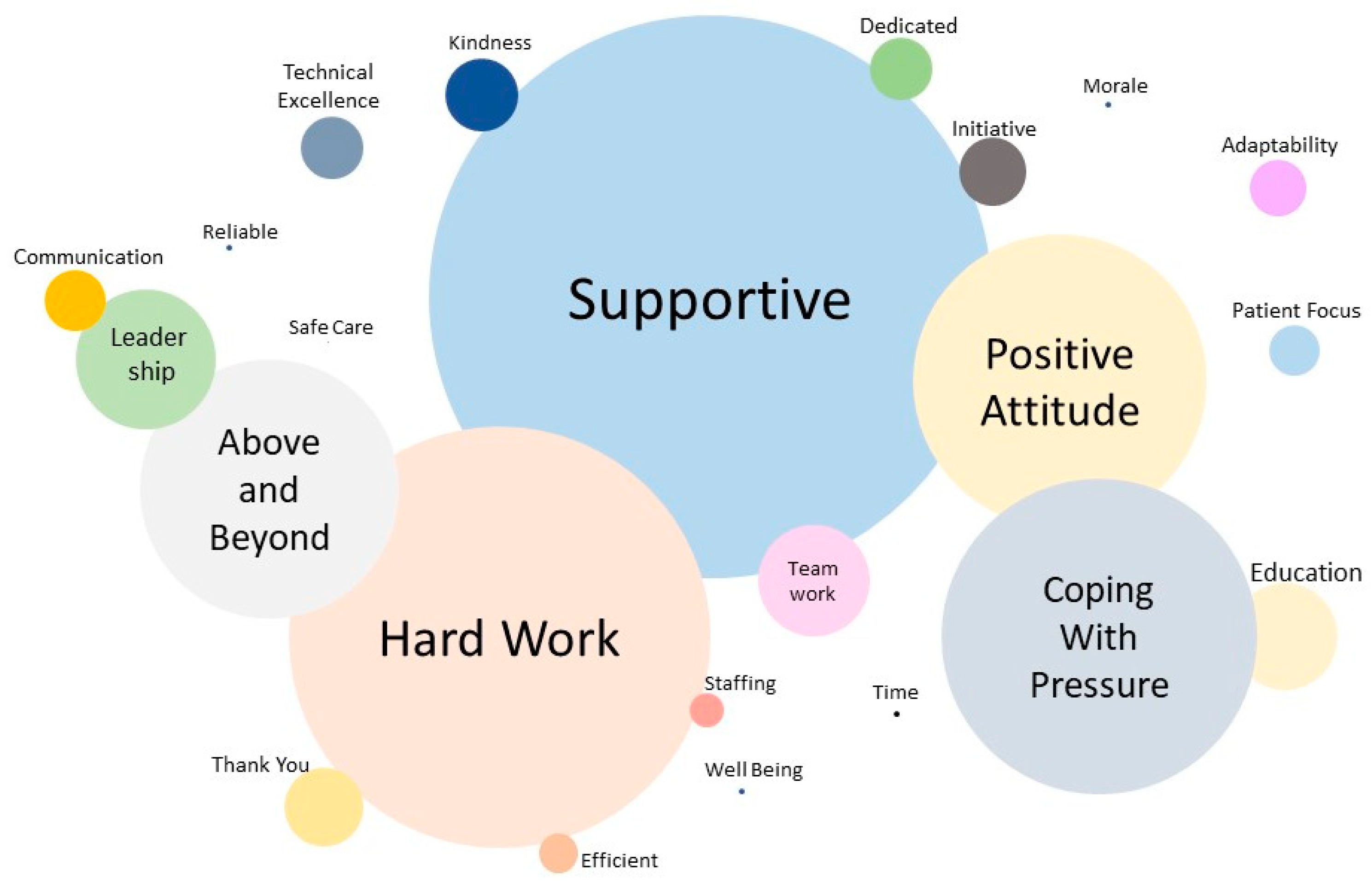
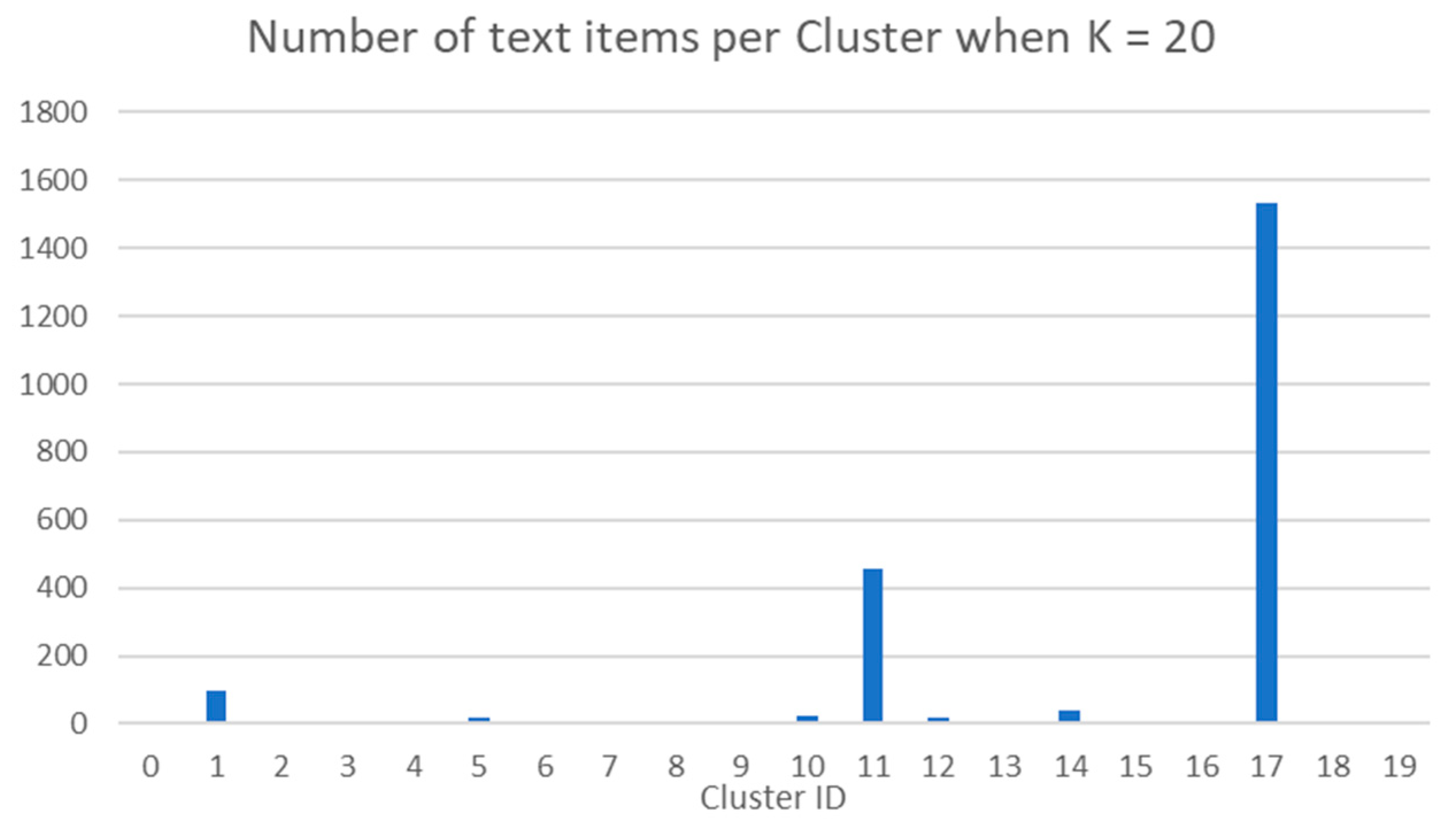
• The distribution of the themes is not balanced. For example, the largest theme “Supportive” is the primary theme for 439 items (19.74%). The smallest theme “Safe Care” is the primary theme for solely 1 item (0.04%). The number of items per category has a standard deviation of 111.23 items. The distribution for the remaining theme categories is also uneven, see Figure 2.
• Since all the text is positive feedback, many of the text items share a similar vocabulary and tone regardless of the theme category to which they belong. For example, the phrase “Thank you” appears in 807 items (36.29%). However, only 61 items (2.74%) belong to the primary theme of “Thank You”.
• The themes are of a subjective nature, dependent on individual interpretation so they could be viewed in different ways. For example, the theme “Teamwork” is not objectively independent of the theme “Leadership”. Thus, there may be some abstract overlap between these themes. Furthermore, there is no definitive measure to determine which theme is more important than another for a given text item, making the choice of the primary theme equally subjective.

Given the classification challenges posed by the LFE dataset, it was important to benchmark results. Thus, all experiments are compared to both well-known text classification datasets and other datasets which share one or more of the characteristics with the LFE dataset.

The first benchmark dataset was the “ApteMod” split of the Reuters-21578 dataset (Reuters). This consists of short articles from the Reuters financial newswire service published in 1987. This split solely contains documents which have been manually classified as belonging to at least one topic, making this dataset ideal for text classification. This dataset is already sub-divided into a training set and testing set. Since k-fold cross validation was used, the datasets were combined. Finally, since multiple themes were not assigned with any order of precedence, items which had been assigned to more than one topic were removed. Although this dataset does not share many of the classification challenges of the LFE dataset, it is widely used in text classification [29,30]. Thus, it provided indirect comparisons with other work in this field.

Three other datasets were chosen since each share one of the characteristics of the LFE dataset.

• The “Amazon Hierarchical Reviews” dataset is a sample of reviews from different products on Amazon, along with the corresponding product categories. Amazon uses a hierarchical product category model, so that items can be categorized at different levels of granularity. Each item within this dataset is categorized in three levels. For example, at level 1 a product could be in the “toys/games” category. At level 2, it could be in the more specific “games” category. At level 3, it could be in the more specific “jigsaw puzzles” category. This dataset was selected as it provides a direct comparison of classification accuracy, when considering the relative dataset volume compared to the number of categories.
• The “Twitter COVID Sentiment” dataset is a curation of tweets from March and April 2020 which mentioned the words “coronavirus” or “COVID”. This dataset was manually classified within one of the following five sentiments: extremely negative, negative, neutral, positive or extremely positive. The source dataset had been split into a training set and a testing set. As with the Reuters dataset, these two subsets were combined.
• The “Twitter Tweet Genre” dataset is a small selection of tweets which have been manually classified into one of the following four high level genres: sports, entertainment, medical and politics.

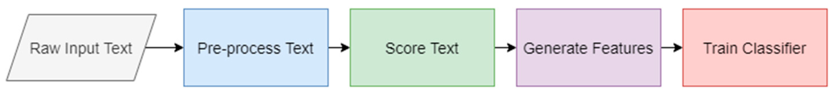
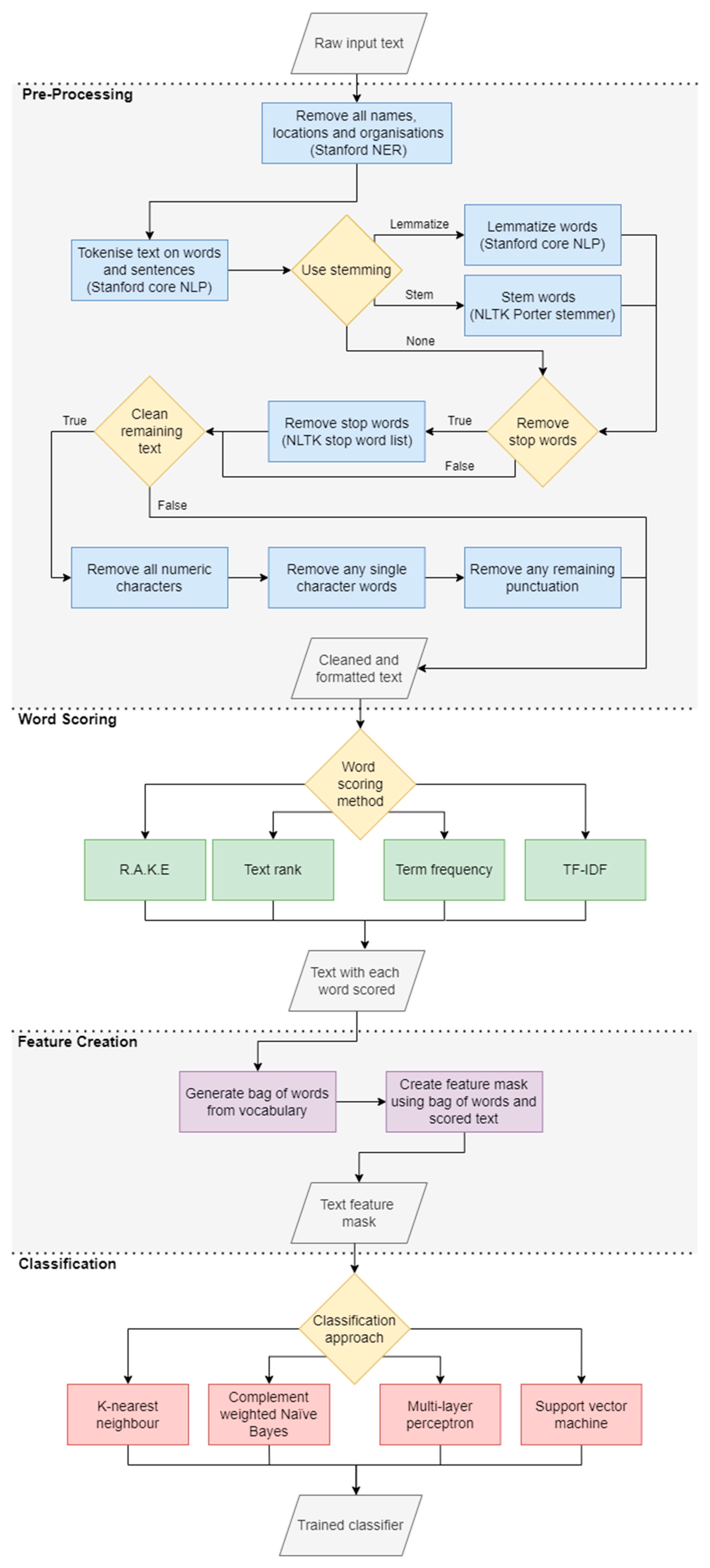
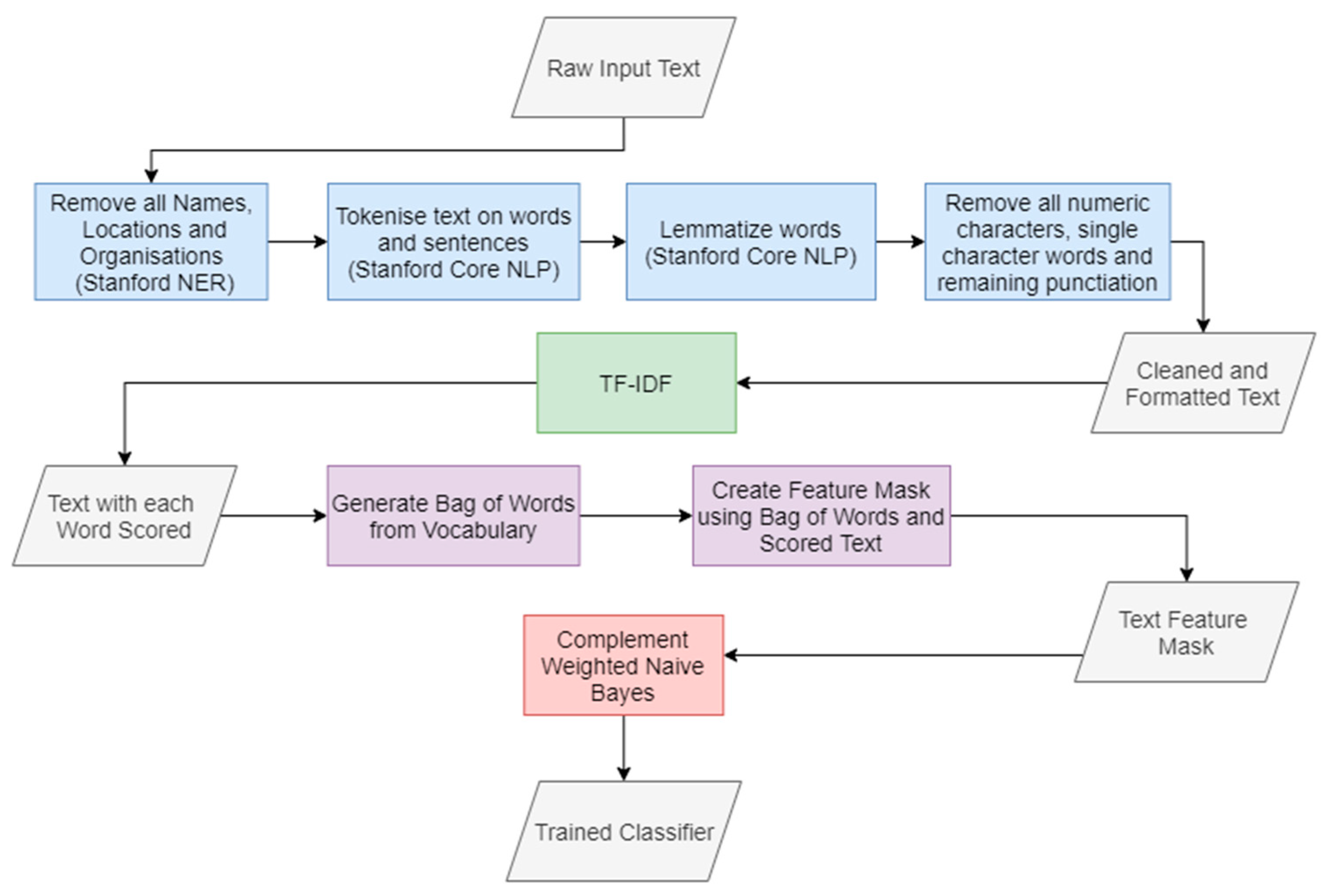
Each of these datasets share some of the complex characteristics of the LFE dataset described at the start of this section.

Table 1. Comparison of the datasets based on the complexity of their classification characteristics. The numbered characteristics refer to the list at the start of this section.

Dataset Name and Shared Characteristics		Description
Reuters	3	There are 9160 documents, classified into one of 65 categories. Average of items per category of 140.90.
	4	The largest category “earn” contains 3923 documents (42.83%). The second largest category “acq” contains 2292 documents (25.02%). The smallest 9 categories only contain 1 document (0.0001%). The number of items per category has a standard deviation of 553.13.
Amazon Hierarchical Reviews	2	The average amount of words in a review is 76.5, with the shortest review 1 containing 1 word and the longest containing 1068 words.
	3	Based on level 3 categorizations, there are 39,999 documents, classified into one of 510 categories. Average of items per category of 78.4.
	5	Since all the text are reviews, there are common words in the vocabulary which have no relation to determining the product category. For example, “great” appears in 9762 reviews (24.41%). However, “great” bears no relation to the product category.
Twitter COVID Sentiment	2	The average number of words in a tweet is 27.8, with the shortest 2 containing 1 word and the longest containing 58 words.
	6	Sentiment analysis in general has a subjective nature to the classifications given [31]. This dataset also has some specific cases where two very similar tweets have been given opposing sentiments, an example can be found in Appendix B.
Twitter Tweet Genre	1	This dataset consists of only 1161 documents.
	2	The average amount of words in a tweet is 16 with the shortest 2 containing 1 word and the longest containing 27 words.

¹ The shortest review in this dataset contains 0 words and only punctuation. However, this was discounted as it was removed during pre-processing and not used. ² Some tweets in this dataset contain 0 words and only URLs, retweets or user handles. However, these were discounted as they were removed during pre-processing and not used.

presents and compares these similarities. The full specification of all the datasets is available in

Table 2. Full specification of datasets. All values presented in this table represent the raw datasets prior to removal of any invalid entries, pre-processing or text cleaning.

Dataset Name	Items	Categories	Avg. Word Count	Avg. Character Count	Avg. Items per Category 1
LFE	2307	24	49.6	290.4	96
Reuters	9160	65	104.4	643.1	140
Amazon Hierarchical Reviews	39,999	6/64/510 2	76.5	424.1	6666/624/78 2
Twitter COVID Sentiment	44,955	5	27.8	176.4	8950
Twitter Tweet Genre	1161	4	16.0	101.9	290

¹ Assuming items were evenly distributed between categories, this is the minimum number of items assigned to each category. ² Multiple values are presented for the Level 1, Level 2 and Level 3 hierarchy of categories, respectively.

.

Currently, the LFE dataset is manually classified by hospital staff, who have to read each text item and assign it to a theme. Therefore, we are the first to experiment with applying automatic text classification to this dataset. The Amazon Hierarchical Reviews, Twitter COVID Sentiment and Twitter Tweet Genre datasets were primarily selected for their similar characteristics to the LFE dataset. However, another advantage they provided was that they contained extremely current data having all been published in 2020 (April, September and January, respectively). Although these datasets were useful for our investigation into how dataset characteristics affect classification accuracy, it was difficult to draw direct comparisons with related work in this field due to the dataset originality. The Reuters dataset was selected because of its wide use in this field as a benchmark, allowing direct comparisons of our novel pipeline results to other well-documented work.

Some of the seminal work in automatic text classification on the Reuters dataset was by Joachims [32]. Through the novel use of support vector machines, a micro averaged precision-recall breakeven score of 86.4 was achieved across the 90 categories which contained at least one training and one testing example. After this, researchers have used many different configurations of the Reuters dataset for their analysis. Some have used the exact same subset but applied different feature selection methods [33], while other work has focused on only the top 10 largest categories [34,35]. Unfortunately, the wide range of feature selection and category variation limits reliable comparison. However, by selecting related work with either (i) similar pre-processing and feature section methods, or (ii) similar category variation, we aim to ensure our proposed pipeline is performing with comparable levels of accuracy.

4. Methodology

For this research, a software package was developed using the Python programming language (Version 3.7), making use of the NumPy (Version 1.19.5) [36] and Pandas (Version 1.2.3) [37] libraries for efficient data structures and file input and output. The core concept was to develop an intuitive data processing and classification pipeline based on flexibility, thus enabling the user to easily select different pre-processing and classification techniques each time the pipeline is executed. As discussed in Section 2, classification often uses a generalized flow of data through a document classification pipeline. The approach presented in this paper follows this model. Figure 3 shows an overview of the pipeline developed.

Since the LFE dataset contained a range of proper nouns which provided no benefit to the classification task, they were removed to optimize the time required for each experiment. The Stanford named entity recognition system (Stanford NER) [38] was used to tag any names, locations and organizations in the raw text. Subsequently, these were removed from the dataset. In total, 3126 proper nouns were removed. A manual scan was performed to confirm that most cases were covered. Some notable exceptions were the name “June” (which was most likely mistaken for the month) and the word “trust” when used in the phrase “NHS trust”. Neither of these were successfully tagged by Stanford NER. The dataset used in this work is the final version with the names, locations and organizations removed.

To maintain similarity in the pre-processing approaches, the Stanford core NLP pipeline [39], provided through the Python Stanza toolkit (Version 1.2) [40], was used where possible. This provided the tools for tokenizing the text, and lemmatizing words. However, Stanford core NLP did not provide any stemming options, so an implementation of Porter Stemmer [41] from the Python natural language toolkit (NLTK) (Version 3.5) [42] was used. NLTK also provided the list of common English stop words for stop word removal. The remaining pre-processing techniques (removal of numeric characters, removal of single character words and punctuation removal) were all developed for this project. The final pre-processing component was used to specifically clean the text of the Twitter collections. This consisted of removing URLs, “#” symbols from Twitter hashtags, “@” symbols from user handles and retweet text (“RT”). This was the final part of the software developed for this project’s source code.

A selection of four word scoring metrics is made available in the pipeline. RAKE [10] was used via an implementation available in the rake-nltk (Version 1.0.4) [43] Python module. A TextRank [9] implementation was designed and developed derived from an article and source code by Liang [44]. An implementation of TF-IDF and a term frequency model were also developed.

Within the stage of feature extraction, the BoW model was developed using standard Python collections. These were originally listed and subsequently converted to dictionaries to optimize the look-up speed when generating feature masks. Feature masks were represented in NumPy arrays to reduce memory overhead and execution time.

All classifiers used in this publication originate from the scikit-learn (Version 0.24.1) [45] machine learning library. This library was selected since (i) it provided tested classifier builds to be used, (ii) a range of statistical scoring methods and (iii) it is a popular library used in similar literature thereby enabling direct comparison with other work in this field. For this project a set of wrapper classes were designed for the scikit-learn classifiers. All classifier wrappers were developed upon an abstract base class to increase code reuse, speed up implementation of new classifiers and ensure a standardized set of method calls through overriding. The base class and all child classes are available in the “Classifiers” package within the source code. A link to the full source code can be found in the Supplementary Materials Section.

Within the final stage of Classification, four of the most common text classifiers are provided. These are k-nearest neighbor (KNN), compliment weighted naïve bayes (CNB), multi-layer perceptron (MLP) and support vector machine (SVM). Tuning the hyper parameters of each of these classifiers, for every dataset, would have produced too much variability in the results. Therefore, each classifier was tuned to the LFE dataset; the same hyper parameters were used on all datasets. When tuning was performed, only one variable was tuned at a time, the remainder of the pipeline remained constant, see Figure 4.

The first classifier, KNN, determines the category of an item based on the categories of the nearest neighbors in feature space. The core parameter to set is the value of k; the number of neighbors which should be considered when classifying a new item. To define k, a range of values were tested, and their accuracy was assessed based on their F1 score. See the full results in Appendix C,

Table A2. KNN tuning: how the F1 score varied (micro and macro averaged) as the value of k was altered. Tests performed using the constant processing pipeline. Selected k value shown in bold.

k	F1 Score (Micro)	F1 Score (Macro)
9	0.205481	0.053783
11	0.215820	0.053813
13	0.223463	0.055129
15	0.223917	0.053341
17	0.227964	0.054558
19	0.232904	0.054457
21	0.230655	0.053048
23	0.242796	0.055268
25	0.241004	0.050718
27	0.238308	0.049159
29	0.230211	0.047173
31	0.232014	0.047116

. The value of k was defined as 23. Work by Tan [46] suggested weighting neighbors based on their distance may improve results when working with unbalanced text corpuses. Thus, this parameter was also tuned. However, when this was applied to the LFE dataset, uniform weighting produced better results. The results of these tests are shown in Appendix C,

Table A3. KNN tuning: F1 score (micro and macro averaged) using uniform weighting compared to distance weighting. Although the F1 macro average score is higher for distance weighing, micro averaging is less susceptible to fluctuations from class imbalance, therefore this was chosen as the deciding factor. Tests performed using the constant processing pipeline. Selected weighting method shown in bold.

Weighting Method	F1 Score (Micro)	F1 Score (Macro)
Uniform	0.242796	0.055268
Distance	0.236509	0.067957

.

The second classifier, Compliment weighted Naïve Bayes (CNB), is a specialized version of multinomial Naïve Bayes (MNB). This approach is reported to perform better on imbalanced text classification datasets, by improving some of the assumptions made in MNB. Specifically, it focuses on correcting the assumption that features are independent, and it attempts to improve the weight selection of the MNB decision boundary. This approach did not require any hyper parameter tuning, and the scikit-learn CNB was implemented as described by Rennie et al. [27].

The third classifier provided is based on the multi-layer perceptron (MLP). There are multiple modern text classification approaches which use deep learning variants of neural networks. Some notable examples are convolutional neural networks (CNN) [47] and recurrent neural networks (RNN) [11], both of which have been used extensively in this field. These approaches have a substantial computational overhead for feature creation. Therefore, deep learning would have been too unwieldly for some of the datasets used in this work. Furthermore, scikit-learn does not provide an implementation of CNN or RNN neural network architectures. Therefore, their use would require another library, reducing the quality of any comparisons made between classifiers. For these reasons, a more traditional, MLP architecture, with a single hidden layer, was used instead. The main parameter to tune for this model was the number of neurons used in the hidden layer. There is much discussion on how to optimize selection of this parameter, but the general rule of thumb is to select the floored mean between the number of input neurons and output neurons as defined below:

$$n_{hidden}=\lfloor \frac{n_{input}+n_{output}}{2}\rfloor$$

The remaining MLP hyper parameters are the default values from scikit-learn and a full list of these can be found in Appendix C,

Table A4. MLP hyper parameter list.

Parameter	Type/Value
Activation function	Rectified linear unit function (RELU)
Weight optimization algorithm	Adam
Max epochs	200
Batch size	64
Alpha (regularization term)	0.0001
Beta (decay rate)	0.9
Epsilon (numerical stability)	1 × 10−8
Early stopping tolerance	1 × 10−4
Early stopping iteration range	10

. The MLP was also set to stop training early if there was no change in the validation score, within a tolerance bound of 1 × 10⁻⁴, over ten epochs.

For the fourth classifier, SVM, it has been reported that the selection of a linear kernel is more effective for text classification problems than non-linear kernels [48]. Four of the most commonly used kernels were tested and confirmed that this was also the case with the LFE dataset. Therefore, a linear kernel was selected for use in this classifier. The results of the tests are found in Appendix C,

Table A5. SVM tuning: F1 score (micro and macro averaged) for different kernels. Although the F1 macro average score is higher for the linear kernel, micro averaging is less susceptible to fluctuations from class imbalance, therefore this was chosen as the deciding factor. Tests performed using the constant processing pipeline. Selected weighting method shown in bold.

Kernel	F1 Score (Micro)	F1 Score (Macro)
RBF	0.241	0.102515
Polynomial (Degree 3)	0.118252	0.026344
Sigmoid	0.369148	0.207289
Linear	0.375895	0.19138

. To account for the class imbalance in the LFE dataset, each class is weighted proportionally in the SVM to reduce bias.

Aside from these supervised classification approaches, an unsupervised model was also developed using scikit-learn and the same classification wrapper class structure. The purpose of this was to examine whether any natural clusters form within the LFE dataset, to enable a wider range of comparisons. K-means [49] was selected as the unsupervised approach, where k represents the number of groups the data should be clustered into. To tune this parameter, two metrics were recorded for a range of potential values of k: the j-squared error and the silhouette score [50]. A lower j-squared error represents a smaller average distance from any given data point to the centroid of its cluster, and a higher silhouette score represents an item exhibiting a greater similarity to its own cluster, compared to other clusters. Therefore, an optimal k value should be minimizing j-squared error whilst maximizing silhouette score. However, j-squared error is likely to trend lower as more clusters are added, leading to diminishing returns for larger values of k. So, it is better suited to examining where the benefit starts to drop off, this is often referred to as finding the “elbow” in the graph.

Appendix C, Figure A1 shows the graph comparing the j-squared error and the average silhouette score for all clusters. From this analysis it was difficult to define the optimal value of k, since the j-squared error trended downwards almost linearly, and the average silhouette score was low for all values of k. Therefore, the LFE dataset was clustered using different small values of k, {2, 8, 13, 16, 20}, which performed better.

5. Results

This research evaluates how fundamental differences in database volume, category distribution and subjective manual classification affect the accuracy of automatic document classification. All experiments were performed on the same computer. It had the following hardware specification: Intel Core i5-8600K, 6 cores at 3.6 Ghz. RAM: 32 GB DDR4. GPU: Gigabyte Nvidia GeForce GTX 1060 6 GB VRAM. The Stanza toolkit for Stanford core NLP supported GPU parallelization, and all experiments exploited this feature. The scikit-learn library did not have any GPU enabled options, so all classification was processed by the CPU.

During experiments, each dataset was tested for the given variables. A fivefold cross validation was used, and the mean score for each validation is reported. If not otherwise stated, all other elements of the pipeline are identical to the constant processing pipeline, described in Section 4. The core metric used for evaluating accuracy was the F1 score, which combines both precision and accuracy into a single measure. This was recorded as both a micro average and a macro average.

Table 3. Evaluates the effect of different pre-processing techniques on the accuracy of classification. The same processing pipeline is maintained aside from pre-processing (TF-IDF, BoW, CNB).

Dataset Name	Pre-Processing	F1 Score (Micro)	F1 Score (Macro)
LFE	None	0.358	0.133
	Stop Word Removal	0.334	0.151
	Word Lemmatizing	0.351	0.136
	Both	0.323	0.153
Reuters	None	0.870	0.477
	Stop Word Removal	0.890	0.526
	Word Lemmatizing	0.858	0.446
	Both	0.886	0.505
Amazon Hierarchical Reviews	None	0.829	0.826
	Stop Word Removal	0.834	0.832
	Word Lemmatizing	0.827	0.825
	Both	0.837	0.833
Twitter COVID Sentiment	None	0.439	0.445
	Stop Word Removal	0.431	0.438
	Word Lemmatizing	0.434	0.438
	Both	0.427	0.434
Twitter Tweet Genre	None	0.800	0.801
	Stop Word Removal	0.786	0.787
	Word Lemmatizing	0.807	0.808
	Both	0.791	0.791

,

Table 4. Evaluates the effect of using different word scoring techniques on the accuracy of classification. The same processing pipeline is maintained aside from word scoring (stop words removal, words lemmatization, additional text cleaning, BoW, CNB).

Dataset Name	Word Scoring Method	F1 Score (Micro)	F1 Score (Macro)
LFE	RAKE	0.152	0.089
	TextRank	0.174	0.045
	Term Frequency	0.342	0.154
	TF-IDF	0.323	0.153
Reuters	RAKE	0.461	0.348
	TextRank	0.597	0.100
	Term Frequency	0.898	0.552
	TF-IDF	0.886	0.505
Amazon Hierarchical Reviews	RAKE	0.381	0.268
	TextRank	0.605	0.573
	Term Frequency	0.834	0.832
	TF-IDF	0.837	0.833
Twitter COVID Sentiment	RAKE	0.213	0.192
	TextRank	0.385	0.364
	Term Frequency	0.435	0.441
	TF-IDF	0.427	0.434
Twitter Tweet Genre	RAKE	0.427	0.422
	TextRank	0.658	0.608
	Term Frequency	0.826	0.827
	TF-IDF	0.791	0.791

and

Table 5. Evaluates the use of different classifiers. The processing pipeline is maintained aside from word scoring (stop words removed, words lemmatized, additional text cleaning, TF-IDF, BoW).

Dataset Name	Classifier	F1 Score (Micro)	F1 Score (Macro)	Fit Time	Score Time
LFE	KNN	0.224	0.053	0.039	0.0758
	CNB	0.323	0.153	0.050	0.0077
	MLP	0.329	0.099	49.029	0.0327
	SVM	0.241	0.102	12.865	2.2606
Reuters	KNN	0.624	0.297	9.618	132.67
	CNB	0.886	0.505	33.872	2.526
	MLP	0.928	0.656	46,840.85	31.941
	SVM	0.771	0.561	49,310.23	35.715
Amazon Hierarchical Reviews	KNN	0.652	0.624	10.831	145.69
	CNB	0.834	0.832	35.250	2.724
	MLP	0.841	0.839	50,840.12	35.769
	SVM	0.822	0.817	56,527.68	39.935
Twitter COVID Sentiment	KNN	0.313	0.302	7.787	149.136
	CNB	0.424	0.431	42.274	2.497
	MLP	0.387	0.384	48,257.21	30.676
	SVM	0.395	0.407	51,774.16	35.027
Twitter Tweet Genre	KNN	0.478	0.405	0.021	0.031
	CNB	0.791	0.791	0.026	0.004
	MLP	0.748	0.748	15.946	0.012
	SVM	0.761	0.765	2.095	0.605

contain the experimental results yielded by the evaluation of changes to the different sections of the proposed pipeline (pre-processing, word scoring and classification respectively). Based on the results from Table 3, Table 4 and Table 5, the optimum pipeline for each dataset was tested and the results can be found in

Table 6. Optimum pipeline result for each dataset with F1 micro averaged score.

Dataset Name	Pre-Processing	Word Scoring Method	Classifier	F1 Score (Micro)
LFE	None	Term Frequency	CNB	0.358
Reuters	Stop Word Removal	Term Frequency	MLP	0.933
Amazon Hierarchical Reviews	Both	TF-IDF	MLP	0.841
Twitter COVID Sentiment	None	Term Frequency	CNB	0.440
Twitter Tweet Genre	Word Lemmatizing	Term Frequency	CNB	0.828

.

To benchmark the accuracy of our pipeline against other related work on automatic text classification,

Table 7. Comparison of the highest achieved micro-averaged score of our pipeline (shown in bold), compared to other published automatic text classification results on the “ApteMod” split of the Reuters-21578 corpus. Accuracy metrics are all F1 scores, except Joachims which is the precision-recall breakeven point.

Automatic Text Classification Approach	Overall Accuracy (Micro-Averaged)
Joachims, T. SVM [32]	0.864
Banerjee, S. et al. SVC [33]	0.870
Ghiassi, M. et al. “DAN2” MLP 1 [34]	0.910
Zdrojewska A. et al. Feed-forward MLP with ADAM [35]	0.924
Haynes, C. et al. Novel Pipeline MLP	0.933

¹ This score is not stated explicitly but was calculated as the average of the F1 testing scores provided in the referenced paper.

presents our results on the Reuters corpus compared to the works mentioned in Section 3.2. As stated in this previous section, it should be noted that a direct comparison of these results is difficult due to the differences in document/category reduction, pre-processing approaches and feature selection. However, the results presented suggest that the approach outlined in this paper produces comparable accuracy to other state-of-the-art approaches.

6. Discussion

6.1. Practical Implications

Based on the results of our experiments we will discuss the two research questions introduced in Section 3.1.

(R1)

The NHS is likely to adopt our approach to automatically classify feedback. This means we have successfully reduced the workload of NHS staff by providing a tool which can be used in place of manual classification. Therefore, the answer to (R1) is positive. Although our proposed classification pipeline attained a lower micro-averaged F1 score on the LFE dataset compared to the benchmark datasets, given the limitations of the dataset, the NHS has found this better than the alternative of manually classifying future datasets.

(R2)

The performance of the classification pipeline published in this paper is evaluated by comparing it against the results of the Reuters dataset with other published work. In this research, a micro-averaged F1 score of 93.30% was achieved. As shown in Table 7, that accuracy outperforms the seminal SVM approaches of Joachims [32], which achieved a micro-averaged breakeven point of 86.40%. Furthermore, the classification pipeline performed in-line with or surpassed more recent approaches [33,34,35]; demonstrating that this classification pipeline produces high accuracy results on other datasets. Therefore, the answer to (R2) is positive.

6.2. Theoretical Implications

Despite the classification pipeline performing very well, the LFE dataset attained a lower micro-averaged F1 score than the benchmark datasets. This discussion will outline the factors which may have caused this result. The four comparison datasets all outperformed the LFE dataset for almost all potential pipeline setups. This suggest that there is an underlying limiting factor, or factors, within the dataset itself. To break down this comparison, each of the characteristics (see Section 3) will be discussed.

• The dataset is relatively small. The overall size of the items in the dataset may have resulted in an advantage to the Reuters and Amazon Hierarchical Reviews results, as it is widely accepted that a larger and more varied dataset will produce better classification results [51,52]. However, the much smaller Twitter Tweet Genre dataset, also achieved a high level of accuracy with a micro-averaged F1 score of 82.80%. Considering the LFE dataset had almost double the number of items, this characteristic alone is unlikely to be the sole cause of the low accuracy results.
• The length of each text item is short. Both Twitter datasets attained vastly different results to the LFE dataset despite the fact they are similarly characterized as being short in length. These Twitter datasets also had considerably shorter average word counts than the LFE dataset and still outperformed it overall. In conclusion, the average length of each text item is unlikely to be a discriminatory characteristic.
• The number of text items per category is small. The average distribution of items per category did not limit performance on the Reuters dataset. However, that could be attributed to the larger overall size, which would have provided more samples for each category in comparison to the LFE dataset.
• The distribution of categories is not balanced. In terms of category distribution, all classification techniques for both the Reuters and LFE datasets suffered from the same issue, where the smallest categories were never applied when classifying the test dataset. Specifically, nine of the Reuters categories and five of the LFE categories never appeared in any of the test classifications. Although this did not impact the overall results of the Reuters classification, the percentage of small categories was much greater in the LFE dataset. In the LFE dataset, 25% of categories comprised less than 1% of the dataset compared with 13.8% in the Reuters dataset. These tiny categories are almost certainly a contributing factor to the lower accuracy of the LFE results.
• All the text is positive. The use of common terms across all categories did not have a significantly negative impact on the classification accuracy of the Amazon Hierarchical Reviews dataset. However, the use of common terms did significantly impact the LFE results. This could be attributed to the fact that each Amazon review had an average word count of more than 50% the average LFE item, resulting in a diluting effect of the repeated common words. Due to the overall larger size of the Amazon Hierarchical Reviews dataset, it had a much larger vocabulary in comparison to the LFE dataset, which may explain why TF-IDF was the optimal scoring method for this dataset.
• The categories are subjectively defined. The subjective nature of both the manual classification and the categories themselves are likely to have played a role in the lower scores for accuracy in both the LFE and the Twitter COVID Sentiment datasets. Although, if the accuracy alone is considered, it is not possible to determine a direct link.

Based on these comparisons, the limiting factors in the LFE classification results are most likely to be (i) the imbalanced category distribution, (ii) the use of repeated common terms across different categories and (iii) the subjective nature of the manual classification. To explore these factors, a manual analysis was performed on the K-means clustering result to see if these same factors were limiting when the LFE dataset was treated as an unsupervised clustering problem, rather than a supervised classification problem.

The first test was used to evaluate how evenly the text items are distributed for different values of k (2, 8, 13, 16, 20 and 150). For any number of clusters, a similar trend emerged, where one cluster would account for between 51% and 98% of all the items. The remaining items were thinly spread between the remaining categories. Figure 5 and Figure 6 depict how the data is unevenly distributed with k values of 20 and 150, respectively. Therefore, there is no evidence of a natural separation for most of the text items in the LFE dataset. Thus, they are either sufficiently generic they get clustered into one large group or that they are overly similar leading to the formation of limited smaller clusters.

To investigate this clustering and to evaluate other limiting dataset characteristics, a manual comparison of the text entries in the small and medium sized clusters was performed. When k = 8, a cluster emerged with only 29, out of the total 2307, items assigned to it. This cluster had a lot of similarities in its text items; almost always congratulating a member of staff on completing a course or gaining a qualification. Words such as “course”, “success”, “level”, “pass” and “congratulations” appeared in this cluster in scales of magnitude higher than across the rest of the clusters. As the value of k varied, this cluster appeared with a 96.6% overlap with a cluster in k = 2, and a 79.3% overlap with a cluster in k = 13.

Furthermore, when k = 8, there was an even smaller cluster identified which contained only 9, out of the total 2307, items. This tiny cluster came from sequential items in the dataset, which share almost exactly the same words. It appears that someone submitted multiple “excellence texts” for a range of different staff. They copied and pasted the same text framework, just changing the name, organization or slightly rewording the text. So, after using the NER, cleaning, lemmatization and removing the stop words, all these items are virtually identical. What is also interesting in this cluster is how the word “fantastic” appeared in every entry whereas it only appears in 5.98% of the whole corpus. This shows one of the downsides to TF-IDF in this case, as words which have no bearing on the classification are getting scored highly due to their rarity across the rest of the corpus. This also supports the argument that common terms, unrelated to the category, could be limiting the classification accuracy. A full breakdown of the occurrence of the most common words in each cluster when k = 8, shown in

Table 8. The percentage of times words appeared in each text item, in each cluster, when k = 8. Only the five largest clusters are shown, since the other three clusters only contained a single item each. Bold values represent statistically significantly values (p < 0.5) in a given cluster when compared to their occurrence in the entire dataset. The case (upper or lower) of the words was not considered.

	Overall	Cluster ID 0	Cluster ID 1	Cluster ID 3	Cluster ID 5	Cluster ID 7
Word/Size	2307	9	1853	319	11	29
Thank	43.44%	100.00%	39.50%	70.22%	0.00%	3.45%
Mentor	1.66%	0.00%	0.81%	6.27%	18.18%	0.00%
Placement	1.57%	0.00%	0.49%	6.58%	45.45%	0.00%
Support	32.10%	0.00%	29.25%	52.04%	36.36%	3.45%
SAU	0.90%	0.00%	0.27%	4.70%	0.00%	0.00%
Work	41.46%	100.00%	43.82%	26.33%	9.09%	55.17%
Hard	15.83%	0.00%	17.00%	7.21%	0.00%	48.28%
Help	31.79%	22.22%	29.30%	50.47%	0.00%	3.45%
Team	32.87%	0.00%	36.97%	13.79%	18.18%	0.00%
Staff	22.84%	0.00%	25.74%	9.72%	0.00%	0.00%
Course	2.52%	0.00%	1.35%	2.19%	0.00%	86.21%
Success	3.33%	100.00%	2.10%	1.88%	0.00%	68.97%
Level	4.90%	0.00%	2.10%	1.88%	0.00%	58.62%
Pass	5.94%	0.00%	6.58%	1.25%	0.00%	20.69%
Patient	37.54%	0.00%	42.31%	15.67%	9.09%	0.00%
Fantastic	5.98%	100.00%	5.45%	3.45%	81.82%	10.34%
Congratulation	1.39%	0.00%	0.38%	0.31%	0.00%	79.31%
Ward	14.12%	0.00%	14.25%	14.11%	27.27%	6.90%

, shows a general theme can be manually identified for most of clusters.

• Placement. Cluster ID 5 has a high prevalence of the words: “placement”, “mentor”, “support” and “team”.
• Course Pass. Cluster ID 7 has a high prevalence of the words: “course”, “success”, “level”, “pass”, “hard” and “work”.
• General Support. Cluster ID 3 has a high prevalence of the words: “thank”, “support” and “help”.

Consider how the large remaining cluster has a similar distribution of words when compared to the full dataset. This suggests that this large cluster is a ‘catch-all’ for all the items not specific enough to be classified elsewhere. This reinforces the conclusion that rarely used but generic terms in the LFE dataset are biasing the accuracy of classification.

This could also explain why the simple scoring metric of term count was optimal for the LFE data. The other single word scoring methods (Text Rank and TF-IDF) both give higher weight to words which are common in a given item, in comparison to the rest of the corpus. However, in this dataset the most commonly used words are actually those that most closely represent the categories:

• “Thank” appears in 43.44% of items.
• “Support” appears in 32.10% of items.
• “Work” appears in 41.46% of items, “Hard” appears in 15.83% of items.

When you consider there are categories specifically for “Thank you”, “Supportive” and “Hard Work”, it is clear these terms being underweighted could be another limiting factor of the LFE dataset. The limiting factor of subjective manual classification is evident in this same analysis. Although “Thank” appears in 43.44% of items, only 2.74% of the items have got a primary theme of “Thank you”. A specific example of this can be seen in one of the text items, after it has been lemmatized and stop words have been removed. Consider the text “ruin humor wrong sort quickly good day much always go help support thank”. This seems quite generic and contains many keywords which might suggest “Supportive” or “Thank you” as the category. However, this text item was manually classified with a primary theme of “Positive Attitude” and a secondary theme of “Hard Work” despite it not having any of the common keywords associated with these themes.

Overall, the data suggest that the common limiting factors of classifying the LFE dataset are also present when it is clustered. Indeed, this means that there is an intrinsic limitation on the ability to classify this specific dataset.

6.3. Future Research

A number of open issues offer opportunities for future work. For example, it would be interesting to evaluate our pipeline with the latest iteration of the LFE dataset, as new entries are added every month. A larger dataset would hopefully provide more instances of different themes and reduce the imbalanced theme distribution.

An alternative option would be to see if the accuracy of our pipeline could be improved on the same dataset if the number of themes was reduced. For instance, some similar themes could be combined such as “Kindness” and “Positive Attitude”, which have a high degree of overlap. Some of the more generic, larger themes could also be removed entirely, for example, “Supportive” and “Hard Work”. Based on the discussion above, it would be expected that this would reduce the imbalanced theme distribution and increase the ratio of text items to themes.

A separate area of research would be improvements to novel pipeline software. Currently, it is a useful tool to test a range of different text pre-processing, word scoring and classification methods to determine which is the most suitable for a given dataset. However, it could be improved if this process was automated, so that the pipeline would test different combinations, rank them and automatically select the most efficient one. To achieve this, the novel pipeline would require a high level of optimization and structure reordering. However, this addition would make this tool more accessible to researchers outside the field, as it would require less inherent knowledge of the processes used.

References

1. Pong, J.Y.-H.; Kwok, R.C.-W.; Lau, R.Y.-K.; Hao, J.-X.; Wong, P.C.-C. A comparative study of two automatic document classification methods in a library setting. J. Inf. Sci. 2007, 34, 213–230. [Google Scholar] [CrossRef]
2. Androutsopoulos, I.; Koutsias, J.; Chandrinos, K.V.; Paliouras, G.; Spyropoulos, C.D. An evaluation of Naive Bayesian anti-spam filtering. In Proceedings of the Workshop on Machine Learning in the New Information Age; Potamias, G., Moustakis, V., van Someren, M., Eds.; Springer: Barcelona, Spain, 2000; pp. 9–17. [Google Scholar]
3. Connelly, A.; Kuri, V.; Palomino, M. Lack of consensus among sentiment analysis tools: A suitability study for SME firms. In Proceedings of the 8th Language and Technology Conference, Poznań, Poland, 17–19 November 2017; pp. 54–58. [Google Scholar]
4. Meyer, B.J.F. Prose Analysis: Purposes, Procedures, and Problems 1. In Understanding Expository Text; Understanding Expository Text; Routledge: Oxfordshire, England, UK, 2017; pp. 11–64. [Google Scholar]
5. Kim, S.-B.; Han, K.-S.; Rim, H.-C.; Myaeng, S.H. Some effective techniques for naive bayes text classification. IEEE Trans. Knowl. Data Eng. 2006, 18, 1457–1466. [Google Scholar]
6. Ge, L.; Moh, T.-S. Improving text classification with word embedding. In Proceedings of the 2017 IEEE International Conference on Big Data (Big Data), Boston, MA, USA, 11–14 December 2017; pp. 1796–1805. [Google Scholar]
7. Zhang, Y.; Jin, R.; Zhou, Z.-H. Understanding bag-of-words model: A statistical framework. Int. J. Mach. Learn. Cybern. 2010, 1, 43–52. [Google Scholar] [CrossRef]
8. Wang, S.; Zhou, W.; Jiang, C. A survey of word embeddings based on deep learning. Computing 2020, 102, 717–740. [Google Scholar] [CrossRef]
9. Manevitz, L.M.; Yousef, M. One-class SVMs for document classification. J. Mach. Learn. Res. 2001, 2, 139–154. [Google Scholar]
10. Ting, S.L.; Ip, W.H.; Tsang, A.H.C. Is Naive Bayes a good classifier for document classification. Int. J. Softw. Eng. Its 2011, 5, 37–46. [Google Scholar]
11. Lai, S.; Xu, L.; Liu, K.; Zhao, J. Recurrent convolutional neural networks for text classification. In Proceedings of the Twenty-ninth AAAI Conference on Artificial Intelligence, Austin, TX, USA, 25–30 January 2015. [Google Scholar]
12. Conneau, A.; Schwenk, H.; Barrault, L.; Lecun, Y. Very deep convolutional networks for text classification. Ki Künstliche Intell. 2016, 26, 357–363. [Google Scholar]
13. Kannan, S.; Gurusamy, V.; Vijayarani, S.; Ilamathi, J.; Nithya, M. Preprocessing techniques for text mining. Int. J. Comput. Sci. Commun. Netw. 2014, 5, 7–16. [Google Scholar]
14. Nothman, J.; Qin, H.; Yurchak, R. Stop word lists in free open-source software packages. In Proceedings of the Workshop for NLP Open Source Software (NLP-OSS), Melbourne, Australia, 20 July 2018; pp. 7–12. [Google Scholar]
15. Jivani, A.G. A comparative study of stemming algorithms. Int. J. Comp. Tech. Appl 2011, 2, 1930–1938. [Google Scholar]
16. Ramos, J. Using tf-idf to determine word relevance in document queries. In Proceedings of the First Instructional Conference on Machine Learning, Citeseer, Banff, AB, Canada, 27 February–1 March 2011; Volume 242, pp. 29–48. [Google Scholar]
17. Mihalcea, R.; Tarau, P. Textrank: Bringing order into text. In Proceedings of the 2004 Conference on Empirical Methods in Natural Language Processing, Barcelona, Spain, 2 July 2004; pp. 404–411. [Google Scholar]
18. Rose, S.; Engel, D.; Cramer, N.; Cowley, W. Automatic keyword extraction from individual documents. Text. Min. Appl. Theory 2010, 1, 1–20. [Google Scholar]
19. Ljungberg, B.F. Dimensionality reduction for bag-of-words models: PCA vs. LSA. Semanticscholar. Org. 2019. Available online: http://cs229.stanford.edu/proj2017/final-reports/5163902.pdf (accessed on 8 February 2022).
20. Cavnar, W.B.; Trenkle, J.M. N-gram-based text categorization. In Proceedings of the SDAIR-94, 3rd Annual Symposium on Document Analysis and Information Retrieval, Las Vegas, NV, USA, 1 June 1994; Volume 161175. [Google Scholar]
21. Ogada, K.; Mwangi, W.; Cheruiyot, W. N-gram based text categorization method for improved data mining. J. Inf. Eng. Appl. 2015, 5, 35–43. [Google Scholar]
22. Schonlau, M.; Guenther, N.; Sucholutsky, I. Text mining with n-gram variables. Stata J. 2017, 17, 866–881. [Google Scholar] [CrossRef]
23. Church, K.W. Word2Vec. Nat. Lang. Eng. 2016, 23, 155–162. [Google Scholar] [CrossRef] [Green Version]
24. Mikolov, T.; Chen, K.; Corrado, G.; Dean, J. Efficient Estimation of Word Representations in Vector Space. arXiv 2013, arXiv:1301.3781. [Google Scholar]
25. Yang, Z.; Yang, D.; Dyer, C.; He, X.; Smola, A.; Hovy, E. Hierarchical attention networks for document classification. In Proceedings of the 2016 Conference of the North American Chapter of the Association for Computational Linguistics: Human Language Technologies, San Diego, CA, USA, 12–17 June 2016; pp. 1480–1489. [Google Scholar]
26. Han, E.-H.S.; Karypis, G.; Kumar, V. Text categorization using weight adjusted k-nearest neighbor classification. In Proceedings of the Pacific-Asia Conference on Knowledge Discovery and Data Mining, Hong Kong, China, 16–18 April 2001; pp. 53–65. [Google Scholar]
27. Rennie, J.D.; Shih, L.; Teevan, J.; Karger, D.R. Tackling the poor assumptions of naive bayes text classifiers. In Proceedings of the 20th International Conference on Machine Learning (ICML-03), Washington, DC, USA, 21–24 August 2003; pp. 616–623. [Google Scholar]
28. Wermter, S. Neural network agents for learning semantic text classification. Inf. Retrieva 2000, 3, 87–103. [Google Scholar] [CrossRef]
29. Yang, Y.; Liu, X. A re-examination of text categorization methods. In Proceedings of the 22nd Annual International ACM SIGIR Conference on Research and Development in Information Retrieval, Berkeley, CA, USA, 15–19 August 1999; pp. 42–49. [Google Scholar]
30. Frank, E.; Bouckaert, R.R. Naive Bayes for Text Classification with Unbalanced Classes. In Lecture Notes in Computer Science; Lecture Notes in Computer Science; Springer: Berlin/Heidelberg, Germany, 2006; pp. 503–510. [Google Scholar] [CrossRef] [Green Version]
31. Liu, B. Sentiment analysis and subjectivity. Handb. Nat. Lang. Process. 2010, 2, 627–666. [Google Scholar]
32. Joachims, T. Text categorization with support vector machines: Learning with many relevant features. In Proceedings of the European Conference on Machine Learning, Bilbao, Spain, 13–17 September 1998; pp. 137–142. [Google Scholar]
33. Banerjee, S.; Majumder, P.; Mitra, M. Re-evaluating the need for modelling term-dependence in text classification problems. arXiv 2017, arXiv:1710.09085. [Google Scholar]
34. Ghiassi, M.; Olschimke, M.; Moon, B.; Arnaudo, P. Automated text classification using a dynamic artificial neural network model. Expert Syst. Appl. 2012, 39, 10967–10976. [Google Scholar] [CrossRef]
35. Zdrojewska, A.; Dutkiewicz, J.; Jędrzejek, C.; Olejnik, M. Comparison of the Novel Classification Methods on the Reuters-21578 Corpus. In Proceedings of the Multimedia and Network Information Systems: Proceedings of the 11th International Conference MISSI, Wrocław, Poland, 12–14 September 2018; Volume 833, p. 290. [Google Scholar]
36. Harris, C.R.; Millman, K.J.; van der Walt, S.J.; Gommers, R.; Virtanen, P.; Cournapeau, D.; Wieser, E.; Taylor, J.; Berg, S.; Smith, N.J. Array programming with NumPy. Version 1.19.5. Nature 2020, 585, 357–362. [Google Scholar] [CrossRef]
37. McKinney, W. Data structures for statistical computing in python. Version 1.2.3. In Proceedings of the 9th Python in Science Conference, Austin, TX, USA, 9−15 July 2010; Volume 445, pp. 51–56. [Google Scholar]
38. Finkel, J.R.; Grenager, T.; Manning, C.D. Incorporating non-local information into information extraction systems by gibbs sampling. In Proceedings of the 43rd Annual Meeting of the Association for Computational Linguistics (ACL’05), Stroudsburg, PA, USA, 25–30 June 2005; pp. 363–370. [Google Scholar]
39. Manning, C.D.; Surdeanu, M.; Bauer, J.; Finkel, J.R.; Bethard, S.; McClosky, D. The Stanford CoreNLP natural language processing toolkit. In Proceedings of the 52nd annual meeting of the association for computational linguistics: System demonstrations, Baltimore, MD, USA, 23–24 June 2014; pp. 55–60. [Google Scholar]
40. Qi, P.; Zhang, Y.; Zhang, Y.; Bolton, J.; Manning, C.D. Stanza: A Python Natural Language Processing Toolkit for Many Human Languages. Version 1.2. arXiv 2003, arXiv:2003.07082. [Google Scholar]
41. Porter, M.F. An algorithm for suffix stripping. Program 1980, 14, 3. [Google Scholar] [CrossRef]
42. Bird, S.; Klein, E.; Loper, E. Natural Language Processing with Python: Analyzing Text with the Natural Language Toolkit; Version 3.5; O’Reilly Media, Inc.: Cambridge, UK, 2009. [Google Scholar]
43. Sharma, V.B. Rake-Nltk. Version 1.0.4 Software. Available online: https://pypi.org/project/rake-nltk/ (accessed on 18 March 2021).
44. Liang, X. Towards Data Science—Understand TextRank for Keyword Extraction by Python. Available online: https://towardsdatascience.com/textrank-for-keyword-extraction-by-python-c0bae21bcec0 (accessed on 15 April 2021).
45. Pedregosa, F.; Varoquaux, G.; Gramfort, A.; Michel, V.; Thirion, B.; Grisel, O.; Blondel, M.; Prettenhofer, P.; Weiss, R.; Dubourg, V. Scikit-learn: Machine learning in Python, Version 0.24.1. J. Mach. Learn. Res. 2011, 12, 2825–2830. [Google Scholar]
46. Tan, S. Neighbor-weighted k-nearest neighbor for unbalanced text corpus. Expert Syst. Appl. 2005, 28, 667–671. [Google Scholar] [CrossRef] [Green Version]
47. Kalchbrenner, N.; Grefenstette, E.; Blunsom, P. A convolutional neural network for modelling sentences. arXiv 2014, arXiv:1404.2188. [Google Scholar]
48. Zhang, W.; Yoshida, T.; Tang, X. Text classification based on multi-word with support vector machine. Knowl.-Based Syst. 2008, 21, 879–886. [Google Scholar] [CrossRef]
49. MacQueen, J. Some methods for classification and analysis of multivariate observations. In Proceedings of the Fifth Berkeley Symposium on Mathematical Statistics and Probability, Oakland, CA, USA, 1 January 1967; Volume 1, pp. 281–297. Available online: https://projecteuclid.org/proceedings/berkeley-symposium-on-mathematical-statistics-andprobability/proceedings-of-the-fifth-berkeley-symposium-on-mathematical-statisticsand/Chapter/Some-methods-for-classification-and-analysis-of-multivariateobservations/bsmsp/1200512992 (accessed on 8 February 2022).
50. Rousseeuw, P.J. Silhouettes: A graphical aid to the interpretation and validation of cluster analysis. J. Comput. Appl. Math. 1987, 20, 53–65. [Google Scholar] [CrossRef] [Green Version]
51. Catal, C.; Diri, B. Investigating the effect of dataset size, metrics sets, and feature selection techniques on software fault prediction problem. Inf. Sci. 2009, 179, 1040–1058. [Google Scholar] [CrossRef]
52. Barbedo, J.G.A. Impact of dataset size and variety on the effectiveness of deep learning and transfer learning for plant disease classification. Comput. Electron. Agric. 2018, 153, 46–53. [Google Scholar] [CrossRef]
Figure 1. Procedural diagram of the processes used in automatic text classification approaches, where rhomboids represent data and rectangles represent processes.
Mathematics 10 00983 g001
Figure 2. Chart of LFE theme category distributions, where the size of a bubble denotes the number of occurrences of each text item for a particular theme category. Note that the position of the bubbles is synthetic, solely used to portray that overlap occurs between themes.
Mathematics 10 00983 g002
Figure 3. Representation of the text processing and classification pipeline, showing each stage described in Section 2. Rhomboids represent data, rectangles represent processes and diamonds represent decisions which can be made modified within the software parameters.
Mathematics 10 00983 g003
Figure 4. Representation of the processing pipeline used for hyper parameter tuning. From the text input all the way through the processes of tokenizing, lemmatizing, additional text cleaning, TF-IDF scoring, BoW modeling, creation of feature masks to the final stage of using the complement weighted naïve bayes classifier.
Mathematics 10 00983 g004
Figure 5. Distribution of LFE dataset when clustered using k-Means where k = 20.
Mathematics 10 00983 g005
Figure 6. Distribution of LFE dataset when clustered using k-Means where k = 150.
Mathematics 10 00983 g006