Article

Constructing Condition Monitoring Model of Wind Turbine Blades

1
Department of Computer Science and Information Engineering, National Taipei University of Technology, Taipei 106344, Taiwan
2
Health Science Center, School of Biomedical Engineering, Shenzhen University, Shenzhen 518037, China
3
National-Regional Key Technology Engineering Laboratory for Medical Ultrasound, Shenzhen University, Shenzhen 518037, China
4
Guangdong Key Laboratory for Biomedical Measurements and Ultrasound Imaging, Shenzhen University, Shenzhen 518037, China
*
Author to whom correspondence should be addressed.
Mathematics 2022, 10(6), 972; https://doi.org/10.3390/math10060972
Submission received: 11 February 2022 / Revised: 12 March 2022 / Accepted: 14 March 2022 / Published: 18 March 2022
(This article belongs to the Topic Machine and Deep Learning)

Abstract

:
Wind power has become an indispensable part of renewable energy development in various countries. Due to the high cost and complex structure of wind turbines, it is important to design a method that can quickly and effectively determine the structural health of the generator set. This research proposes a method that could determine structural damage or weaknesses in the blades at an early stage via a model to monitor the sound of the wind turbine blades, so as to reduce the quantity of labor required and frequency of regular maintenance, and to repair the damage rapidly in the future. This study used the operating sounds of normal and abnormal blades as a dataset. The model used discrete wavelet transform (DWT) to decompose the sound into different frequency components, performed feature extraction in a statistical measure, and combined with outlier exposure technique to train a deep neural network model that could capture abnormal values deviating from the normal samples. In addition, this paper observed that the performance of the monitoring model on the MIMII dataset was also better than the anomaly detection models proposed by other papers.

1. Introduction

In recent years, due to the rising awareness of environmental protection and the increasingly serious phenomenon of global warming, countries have begun to develop various renewable energy sources, such as solar power, wind power, and hydropower. Among them, wind power is currently the most mature technology and the largest source of renewable energy. Taking Taiwan’s current development of wind power generation as an example, the Ministry of Economic Affairs has proposed that offshore wind turbines in Taiwan will reach a capacity of 5.7 GW in five years, with an annual carbon reduction of 11.92 million metric tons. However, how to maintain offshore wind turbines has become a great concern.
Damaged blades are the cause of the high maintenance cost of wind turbines [1]. At present, a traditional testing method for blades includes ultrasonic testing (UT), acoustic emission (AE) testing, and other technologies that need to be performed by professional technicians under shutdown conditions. Liu et al. [2] mentioned that, for condition monitoring and fault diagnosis (CMFD) of wind turbine blade bearings, one of the main difficulties is that the rotation speeds of blade bearings are very slow. Latoufis et al. [3] suggested that the main challenge for AE analysis is that the fault signals are mingled with heavy noise, which results in expensive maintenance costs. In particular, offshore wind turbines must withstand the erosion of natural phenomena, such as salt and ocean currents under high-temperature and high-humidity environments. This makes the cost of traditional regular maintenance even more expensive. Effective preventive maintenance is planned and scheduled based on real-time data insights [4,5,6], which will be an important issue.
In order to solve the above problems, this paper proposes a monitoring model integrating DWT and a deep neural network (DNN) that could detect wind turbine blade damage without stopping the turbine, thereby achieving the effect of early repair, preventing blades from breaking in the future.
The rest of this paper is organized as follows: Section 2 introduces the literature and neural network architecture related to wavelet transformation and anomaly detection. Section 3 introduces the overall architecture and process of the monitoring model. Section 4 introduces the experimental results. Section 5 is the conclusion of this paper.

2. Related Work

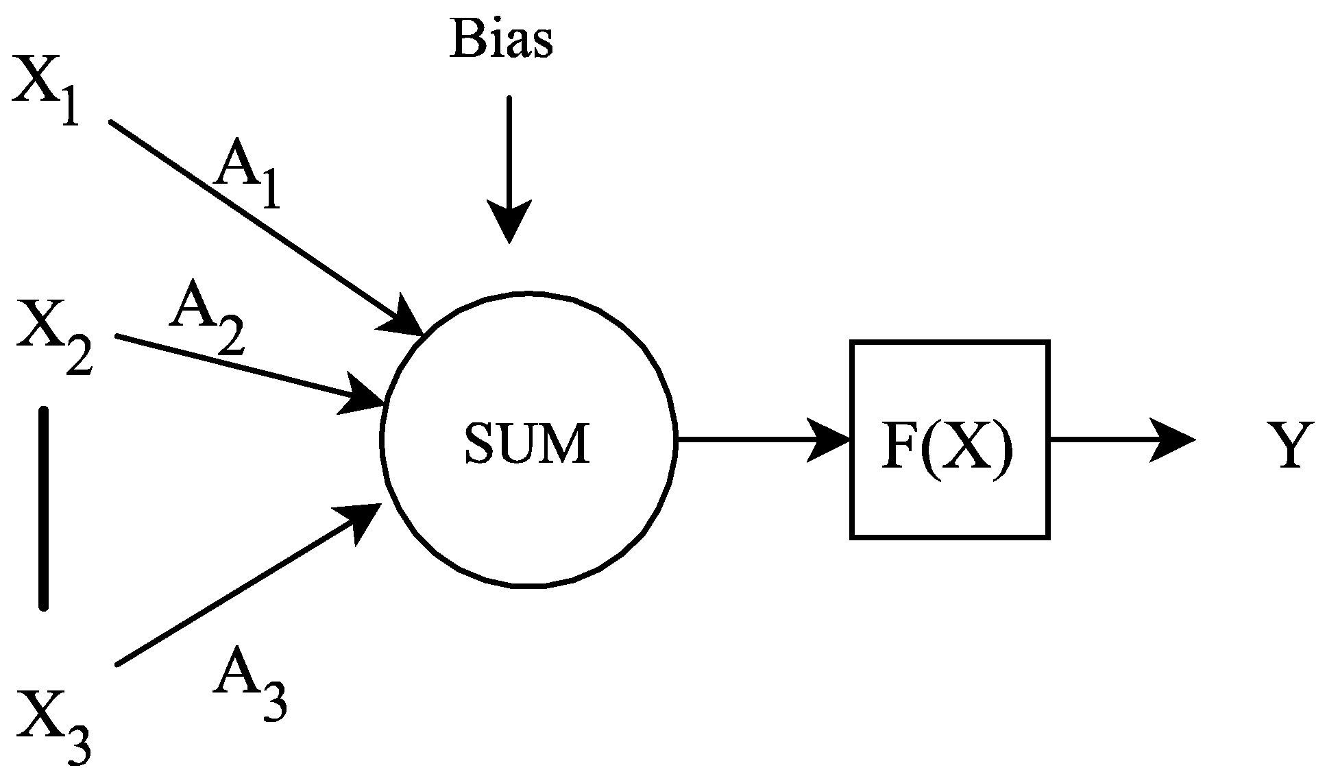
2.1. Deep Neural Network

The basic structure of a DNN consists of an input layer, multiple hidden layers, and an output layer, then a neural network layer is composed of several neurons and a complete neural network structure is formed by stacking network layers on each other. The structure of a single neuron is shown in Figure 1. The neuron is multiplied by the weight vector for each unit in the current layer producing the weighted sum. After adding the bias of the neuron, the input value is calculated by the activation function F(x) to get the output value of the neuron.
A neural network can be categorized into three layers: an input layer, an output layer, and a hidden layer. The input layer serves as the entrance of the entire network and is responsible for receiving data samples for learning. The output layer serves as the final output result of the entire model. The hidden layer provides the ability of the neural network to process and solve the target task.

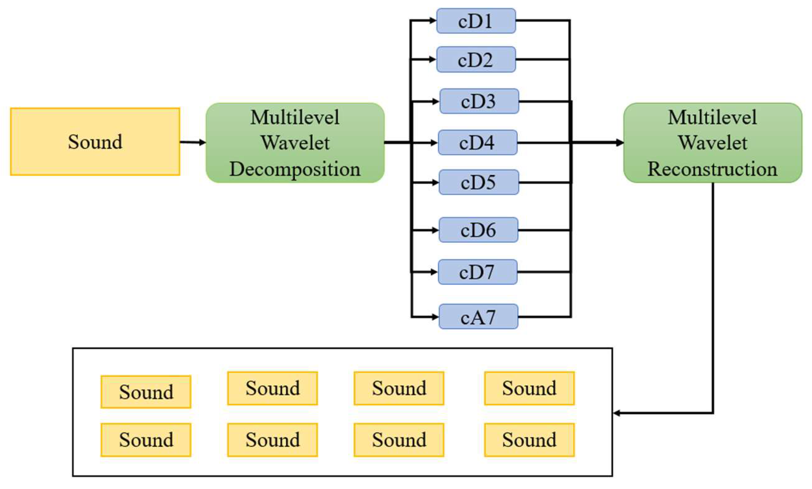
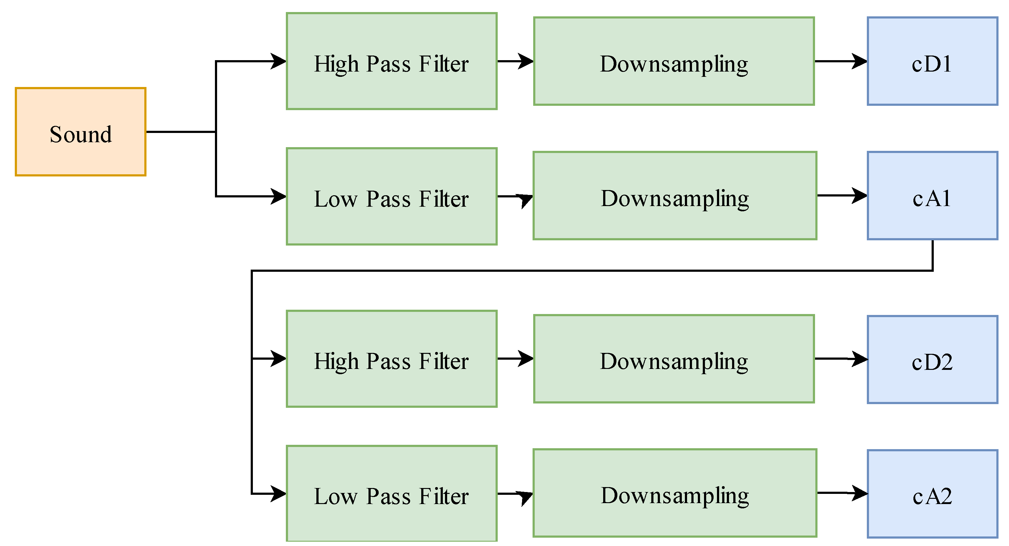
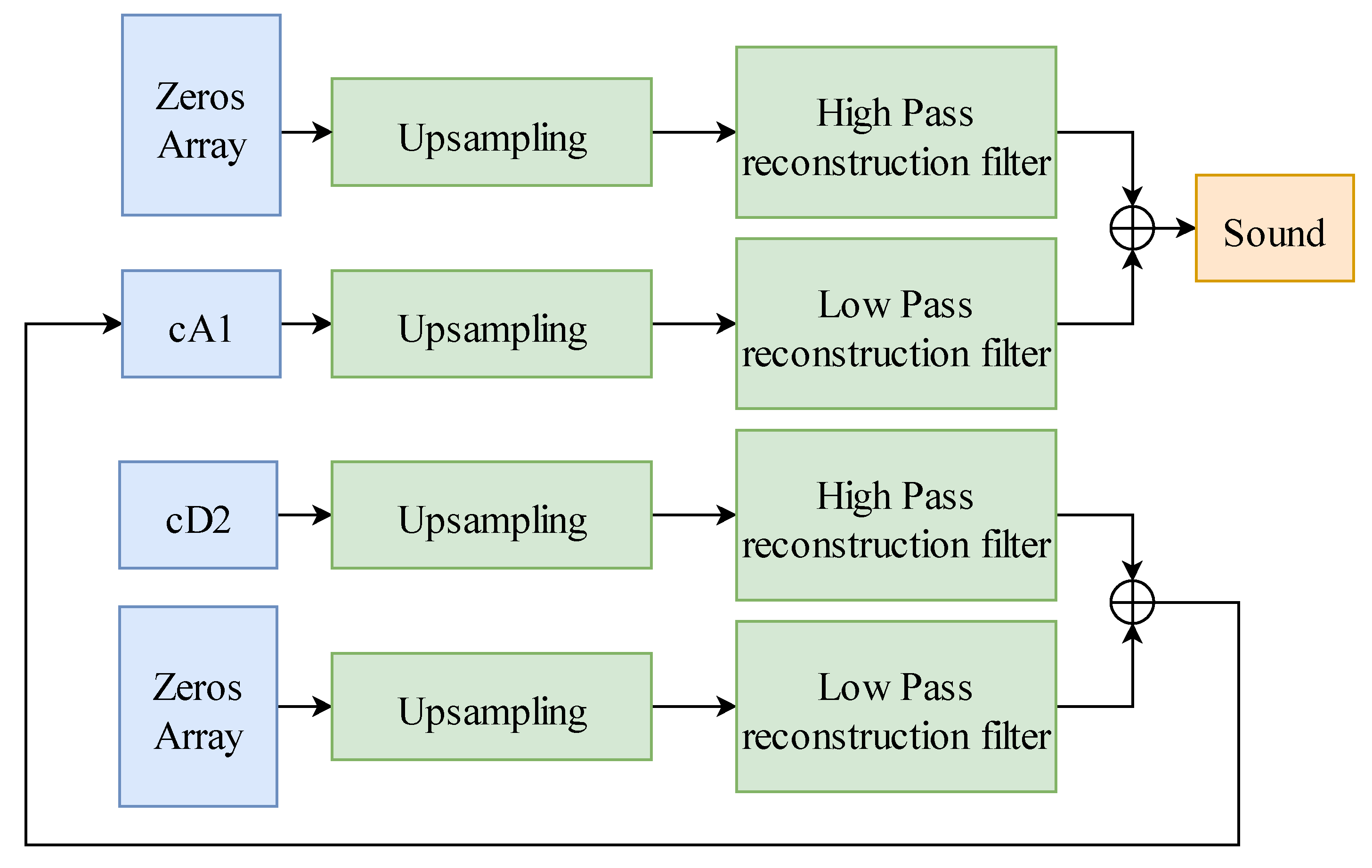
2.2. Wavelet Transform

As shown in Equation (1), the core concept of wavelet transformation is to use a mother wavelet function ψ(t) and a scaling function ϕ(t) to scale or translate the original audio wave, thereby generating various sub-wavelet functions ψ a , b ( t ) and using these as a basis to fit the original audio wave shape. There are two categories in wavelet transform: continuous wavelet transforms and discrete wavelet transform. The difference depends on whether scaling factor a and translation factor b in Equation (1) are in a continuous or discrete distribution:
ψ a , b ( t ) = ψ ( t b a )
Mallat proposed Mallat’s pyramid wavelet decomposition algorithm [7], which introduced the concept of wavelet transform into multi-resolution analysis [7]. Multi-resolution analysis examines the characteristics of the original information by decomposing the information into components of different scales. The analysis of a single resolution may change the characteristics of the information obtained by the analysis due to changes in the original information. For example, images may show different target proportions due to different focal lengths and resolutions. Audio files may confuse the target information due to factors such as recording volume and environmental noise. Through MRA (multi-resolution analysis), the interference of variables that are not related to the target characteristics can be reduced to a certain extent.

2.3. Anomaly Detection

Anomaly detection can be divided into supervised and unsupervised methods based on whether it is necessary to use abnormal samples for model training. Jia et al. [8] proposed a supervised method for use on California traffic flows under normal conditions and abnormal conditions, such as car accidents and road construction, to train the long short-term memory network (LSTM).
Saufi et al. [9] proposed a supervised anomaly detection architecture that can achieve a certain prediction accuracy in the context of limited data, a proper hyperparameter selection method in an SSAE network using a particle swarm optimization algorithm. The spectrum is used as the input, and prediction is made through a stacked sparse autoencoder (SSAE). In particular cases, the prediction accuracy can be higher than 94% using only one sensor. The proposed method has high efficiency but the accuracy is slightly lower than that found in relative research. Consequently, they devised an alternative approach for architecture using the fast kurtogram (FK) method to process the original signal. Compared to other time-frequency transformation methods, such as short-time Fourier transform (STFT), wavelet transform (WT), and empirical mode decomposition (EMD), the FK method has the advantage of not requiring set parameters. In this research, the team did not combine the data collected from multiple sensors; instead, they chose the sensor with the best prediction accuracy as the result.
Each anomaly category in supervised anomaly detection requires a large dataset of balanced data. Yang et al. [10] proposed a data generation method based on a generative adversarial network (GAN) to resolve this issue. To solve the problem of dataset imbalance, the team collected data through three accelerometers and then used fast Fourier transform (FFT) for preprocessing to obtain the real spectrogram data and, at the same time, generated more anomaly data using GAN. After sorting out these two different datasets, a balanced dataset could be obtained. In addition, the team proposed a multiscale convolutional neural network (MSCNN) to construct the anomaly detection model for a harmonic drive. MSCNN is an improved convolutional neural network (CNN) with an additional multiscale coarse-grained layer that can extract features with different scales from the signal data, thereby achieving better prediction accuracy. In the case of unbalanced datasets, the multi-class anomaly classification accuracy is as high as 98.49%. However, the proposed method in this study needs to train MSCNN and GAN separately, so it requires more computing resources and makes it difficult to be directly applied in real industrial environments.
The disadvantage of the supervised machine learning task is that it requires a large number of manually labeled datasets and suffers from potential human bias interference. Kong et al. [11] proposed an architecture combining attention-based recurrent neural networks and an autoencoder. The architecture can automatically find the most valuable features through unsupervised learning and can directly use the original vibration signal as the input instead of using data processed by time-frequency conversion. The proposed architecture makes predictions through the combined weights of the two network architectures. The accuracy of the architecture for rotating machinery anomaly detection was as high as 99.88%, which was 8–10% higher than the CNN mechanism. At the same time, the architecture could be used for other anomaly detection tasks. However, in this article, the proposed method did not include heavy noise handling.
In [12], Mel-frequency cepstral coefficients (MFCCs) were used to train an autoencoder (AE) to achieve an unsupervised anomaly detection method. Some researchers have begun to think about whether they can use other easily available data to replace abnormal samples. Outlier exposure (OE), proposed by Hendrycks et al. [13], uses a model that is trained on an auxiliary dataset of outliers. It was found that the performance of the model trained by this method was higher than that for models trained using normal samples.

2.4. Structural Health Monitoring

Structural health monitoring mainly discusses how to evaluate the structural safety of a structure, the damage to a structure, and the subsequent impact on the reliability of the structure. This method mainly analyzes the health of a structure through non-destructive testing methods. It can be divided into four stages [14]: (1) detection, based on locating any information containing structural damage; (2) positioning, based on identifying the location of damage using the information collected by the detection; (3) evaluation of the severity and repairability of the damage; and (4) prediction of the prognosis and remaining service life of the structure.

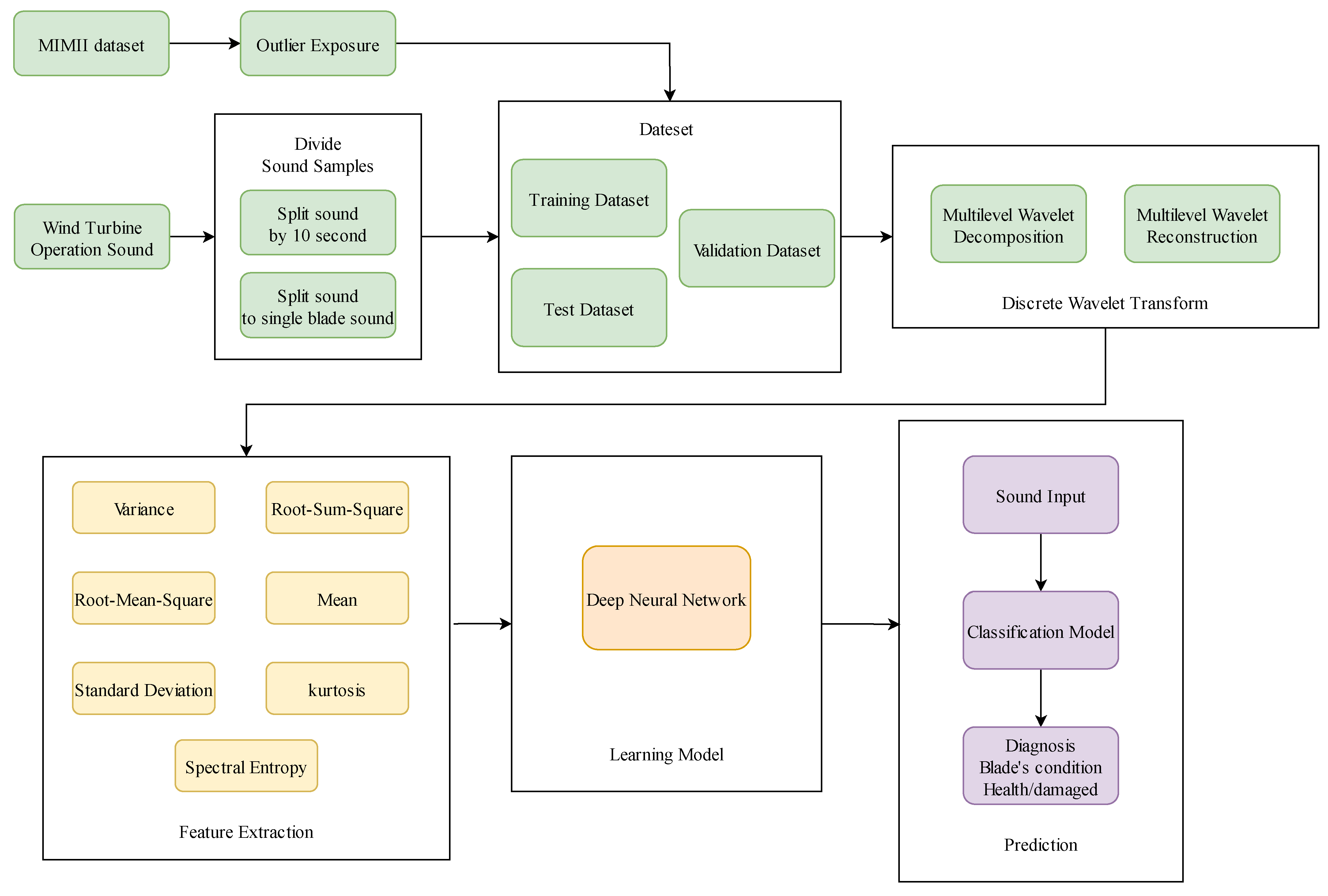
3. The Proposed Approach

This section introduces the architecture and processing flow of the monitoring model. In Section 3.1, the model architecture is introduced. In Section 3.2, the data pre-processing flow of the monitoring model is introduced. The DNN architecture is introduced in Section 3.3.

3.1. Monitor Model Architecture Diagram
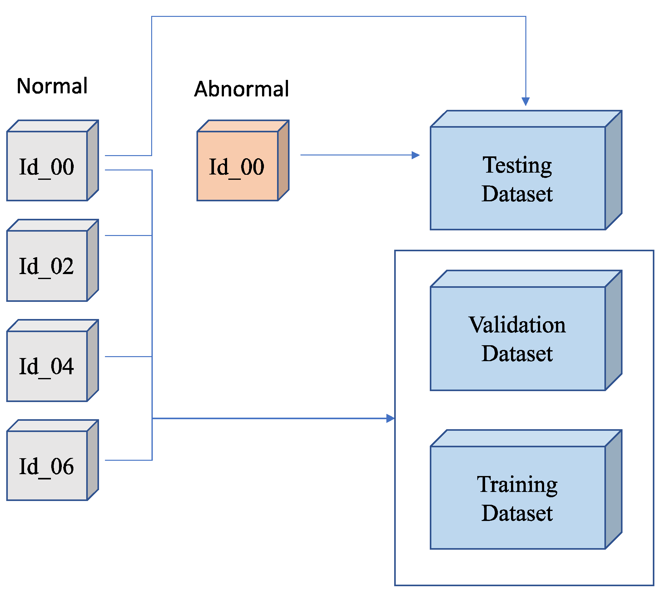
The design process of this paper’s monitoring model architecture is shown in Figure 2. This paper used two datasets to evaluate the effectiveness of the model: the recording files of the mechanical noise generated by operating the wind turbines and the MIMII dataset [12]. For the MIMII dataset, the outlier exposure method was used to create the training set. In the blade sound features part, data pre-processing was performed first by segmenting the blade recordings to increase the number of samples. After segmentation, discrete wavelet transform (DWT) was performed for each recording sample. Each sample was decomposed into a total of eight audio signals with different frequency intervals so that the model could analyze the information contained in different frequencies. Finally, we calculated the mean, variance, root mean square, root sum square, standard deviation, sample kurtosis, and spectral entropy of each audio signal as the feature vectors required by DNN, and concatenated the feature vectors of each audio signal to a 56-dimensional feature vector.
After data pre-processing, the structure of the DNN model was defined. The training process used the Adam optimization algorithm. At the same time, batch normalization and L2 regularization were used to avoid overfitting, and learning rate decay and batch size scaling large batch training were used.

3.2. Dataset

Two different datasets were used in this research—the MIMII dataset and the wind turbine dataset. We used the MIMII dataset to evaluate the anomaly detection performance of the proposed method at first, then used the wind turbine blade dataset to train the model to reach the goal of monitoring turbine blade damages.
The MIMII dataset [12] includes four common industrial machinery types, such as valves, pumps, fans, and slide rails. Each type of machinery was divided into seven different product models and recorded for 10 s at a distance of 50 cm from the machinery through an array microphone. In addition to the sound samples of the normal operation of the machinery, the dataset also recorded samples of abnormal conditions by adding different types of faults to the machinery, such as clogged valves, damaged fan bearings, etc.
To make the sound samples closer to the actual factory operating environment, Purohit et al. [12] used the background noise obtained from the factory recording and the machine sound to synthesize three kinds of data, for which the SNR values were 0 dB (Lin), −6 dB (Lin), and 6 dB (Lin).
The wind turbine blade dataset was collected by our research members; we used highly sensitive recording devices to acquire the sound raw data, then let the domain experts mark the dataset according to whether the blades had cracked. The type of anomaly only included crack blades.
The detail of the blade sounds recording process is as below, the wind turbine models were Enercon E70-7 and Gamesa G80-2MW, recorded as 32-bit audio clips at 44.1 kHz, mono-channel audio. The signal-to-noise ratio (SNR) of the samples was −11.7 dB (Lin). Recording devices were kept at a distance of 67 m from the blades.

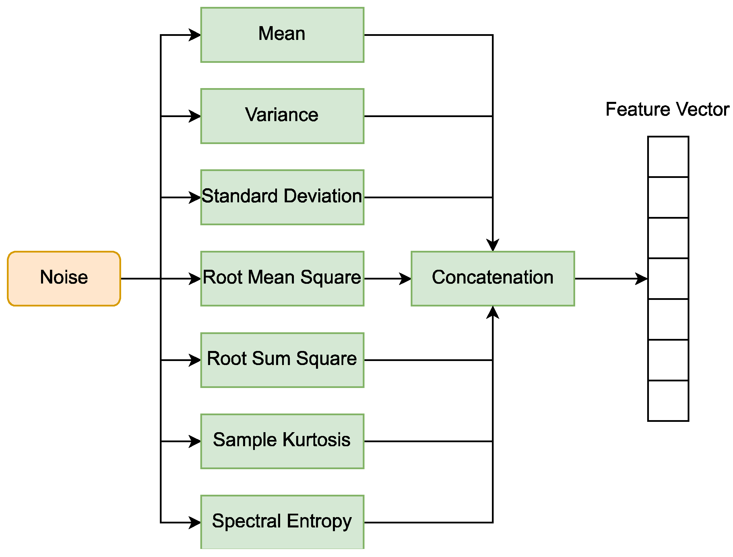
3.3. Data Preprocessing

This paper used two different methods to segment sound raw data in the wind turbine blade dataset: a fixed-length segmentation experiment on a sound file with a length of 10 s and a segmentation experiment in which the original sound was segmented into individual blade sounds. The number of samples in the fixed-length segmentation experiment is shown in Table 1.
For the single-blade segmentation experiment, this paper categorized each blade sound segmented from the whole original sound as either a normal or abnormal blade sound. The number of individual samples is shown in Table 2.
After segmentation, this paper used DWT for denoising by decomposing the original audio into components with different frequency intervals.
The audio decomposition process is shown in Figure 3. Firstly, the sample was decomposed using seven-level discrete wavelet decomposition to get seven detail coefficients and one approximation coefficient. The detail coefficient represented a higher frequency relative to the approximate coefficient, and the approximate coefficient represented the low-frequency component of the signal. After decomposition, each coefficient was reconstructed by wavelet reconstruction. After wavelet reconstruction, eight audio files with different frequency ranges remained.
The filter used in this paper was constructed by the Sym10 wavelet in the symlet wavelet family. Figure 4 is a diagram of the multi-level wavelet decomposition. Taking level 2 as an example, the original audio x[n] is a fixed-length one-dimensional real number array that passes through a high-pass filter (h[k]) of length K and a low-pass filter (g[k]) to separate the high-frequency signal component and the low-frequency signal in Equations (2) and (3):
cA 1 [ n ] = k = 0 K 1 x [ n + 1 k ] g [ k ]
cD 1 [ n ] = k = 0 K 1 x [ n + 1 k ] h [ k ]
Next, the signal component is subjected to a down-sampling filter with a down-sampling factor of two to obtain the first level of detail and approximate coefficients cD1 and cA1.
After the end of the first level, the approximate coefficient, cA1, is used as the input audio in the second level to execute a single-level wavelet decomposition to obtain the two-level coefficients cD2 and cA2. Therefore, the audio investigation will obtain the coefficient set S = {cD1, cD2, cD3, cD4, cD5, cD6, cD7, cA7} after seven stages of wavelet decomposition, which represents the signal components of the original audio files.
The next stage is signal reconstruction. Figure 5 is a diagram of the reconstruction process. Here, only the audio of a specific frequency is retained. Therefore, when performing wavelet reconstruction, except for the coefficient to be reconstructed, the other missing correlation coefficients are used with zeros substituted into the array to complete the reconstruction. As an example, Equation (4) represents the reconstruction of the signal component of the second-level cD2 detail coefficient as an example:
cA 1 [ n ] = k = 0 K 1 cA 2 [ n + 1 k ] g * [ k ] + k = 0 K 1 cD 2 [ n + 1 k ] h * [ k ]
After the cD2 and the approximate coefficients are increased via an upsampling filter with an upsampling factor of two, they are added through the high-pass and low-pass reconstruction filters, h*[k] and g*[k], to obtain the first level approximation coefficient cA1. After that, single-level wavelet reconstruction is performed to restore the signal component of cD2 to the original audio type. By performing seven-level wavelet reconstruction on each coefficient element in coefficient set S, we can obtain eight signal components of the original audio in different frequency intervals.
Finally, the statistical indicators of the audio are calculated and composed as the input feature vector of the DNN model. Statistical indicators are calculated for each time-series audio component to obtain the mean, variance, standard deviation, root mean square (RMS), root sum square (RSS), spectral entropy (SE), sample kurtosis, and a total of seven values as features of the component, as shown in Equations (5)–(11). Suppose time-series signal X is a one-dimensional array of length n, mean M can be calculated using Equation (5).
M = i = 1 n x i n
V a r = i = 1 n ( x i μ ) 2 n
S = i = 1 n ( x i μ ) 2 n
In Equations (6) and (7), V a r is the variance of the audio file and S is the standard deviation. Both use the mean μ to obtain the values for V a r and S.
RMS = i = 1 n ( x i ) 2 n
RSS = i = 1 n ( x i ) 2
kurtosis = i = 1 n ( x i μ ) 4 n V a r ( x ) 2 3
SE = i = 1 n P ( i ) l o g 2 P ( i )
In Equation (11), P ( i ) is the power spectral density.
After calculating the seven statistical indicators of each time-series component, the program concatenates the features of each time-series component into a seven-dimensional vector, as shown in Figure 6.
The vectors of all components are then concatenated from high frequency to low frequency in sequence. Finally, a 56-dimensional feature vector is achieved, which is then used as the input of the DNN model.

3.4. Neural Network Architecture

This paper used a deep neural network to build a machine learning model for training. The model architecture is shown in Table 3. Size represents the number of neurons in the network layer, and activation represents the activation function used in this layer. The first layer has 56 input neurons as the input of the neural network. The neurons in the hidden layer will gradually decrease. Hidden layer activation function uses ReLU, and batch normalization is interspersed between the hidden layers. The last layer has an output neuron in the output layer, and its activation function uses the sigmoid function. All hidden layers use L2 regularization, and the regularization parameter is 0.01.

4. Experiment

This section introduces the experimental process and results. Section 4.1 describes the network model used and compared in the experiment and the learning parameters of the training process. Section 4.2 describes the process of using the classification accuracy and AUC to evaluate the difference between the model’s performance and the experimental results.

4.1. Experimental Process

This paper compared the monitoring model constructed using discrete wavelet transform and fully connected DNN with the monitoring model constructed using a log-mel spectrogram and the convolutional neural network (CNN) model in [15]. The CNN model was tested with ResNet18 and ResNet50, respectively. The window function length of the log-mel spectrogram was 1024, the overlap length was 512, and the Mel frequency bandwidth was 64. The number of iterations for the training process was set to 200 rounds, and the model parameters with the lowest loss of the validation set were saved as the model in the final test stage. The Adam algorithm was used for optimization, the learning parameter β was 0.9, β2 was 0.999, and the learning rate decay was set. After every 10 epochs, if the loss of the validation set changed by less than 0.001, the learning rate was 0.9. The batch size was set at 32 in the MIMII dataset and five in the wind turbine audio dataset.

4.2. Experimental Result

This study used the MIMII dataset to train the monitoring model and compare the experimental results with the best experimental results [12,16,17] to measure the ability of anomaly detection. As the related experiments did not use abnormal samples in the training process, in order to make the benchmark as close as possible, this study referred to [13,18] to train the model using the outlier exposure method.
As shown in Figure 7, for each model of each different machine type, all abnormal samples and the same number of normal samples were taken as the test set. For the training set, the remaining normal samples were combined with normal samples taken from different models of the same machine type, and normal samples of other models were regarded as abnormal samples. The AUC experimental result comparison between the methods used in this research and other models is shown in Table 4.
From Table 4, it could be found that the average AUC of the monitoring model proposed in this study was better than ResNet18 and ResNet50. However, in the training stage, the time cost of the monitoring model in this paper was less than 50% of that for other models, as shown in Table 5.
In this study, the monitoring model constructed by wavelet transform and fully connected layer neural network and the monitoring model constructed by Mel log-spectrogram and CNN model have been used for comparison [15]. The CNN model was tested using ResNet18 and ResNet50, respectively. Table 6 is the comparison between the experimental results of this study and the CNN model [12]. It can be seen from the table that the monitoring model proposed in this research had the best average AUC among the four different machine structures. The results indicate that, in the face of different materials and architectures, the monitoring model could still maintain better prediction accuracy. Among the four types of machines, only the AUC of the slider was lower than the experimental results of the others. This may be because the resolution of the discrete wavelet transforms in the high frequency range was lower and the frequency range was low, which made it difficult for the extracted sound features to retain the complete characteristics of the slider in an abnormal state and resulted in a lower AUC.
The overall monitoring also suggests that the model proposed in this study has an accuracy of 98% and AUC of 0.99 in judging whether the fan contains abnormal blades, and 96% accuracy and AUC of 0.96 in judging whether a single blade is abnormal, which can effectively distinguish whether there is an abnormality in the fan blades.
On the other hand, for the MIMII dataset, the average AUC index of the model was also higher than the abnormality detection model proposed by other researchers.
In this study, the operating sounds recorded from actual operating wind turbines were used for training. Of the data, 60% of the normal samples and abnormal samples containing blade damage were taken as the training set, 20% were taken as the validation set, and 20% were taken as the test set. The fixed-length segmentation experiment result is shown in Table 7.
The accuracy of the monitoring model on the test set was 98.04%, and the AUC was 0.99. On the whole, the monitoring model proposed in this study could indeed effectively distinguish whether the wind turbine contained damaged blades.
The single-blade segmentation experiment was used to test whether the model could classify an abnormal blade sound with damage. The single-blade segmentation experiment results are shown in Table 8.
In terms of the model performance, the accuracy of the monitoring model in this study was higher than ResNet18 and lower than ResNet50, while the AUC was higher than ResNet18 and slightly lower than ResNet50. Overall, the monitoring model of this study could effectively diagnose a blade’s health status using the sound wave data of a single blade. Considering that the model architecture and complexity of this study were much simpler than those of the other two models, the performance of the monitoring model could be improved by trying different network models.

5. Conclusions

This research combined discrete wavelet transformation with deep neural networks to construct a model that could monitor wind turbine blade damage from the running sound. Statistical methods, such as RMS and RSS, were used to extract features, which greatly reduced the complexity and training time of the network models. Discrete wavelet transformation was used to decompose the original audio into components of different frequency ranges, and the neural network self-learned and analyzed the key signal information. Finally, the outlier exposure method was used so that the model would not need to use abnormal samples for training.
With the growth of the scale of wind power generation, the large number of land-based and offshore wind turbines have made it difficult for maintenance manufacturers to follow traditional high-cost manual inspection and repair procedures. The automatic monitoring of the health of the blades through the monitoring model could ensure that damage is repaired at an early stage, thus avoiding the deterioration of the wind turbine structure due to damage over time. In addition, for various machines with special operating sounds, the monitoring model could also properly distinguish whether a machine is operating normally or not.
The monitoring model of this study was based solely on the operating sound of the machine as the source for structural damage judgment. If the damage to the machine does not impact the operating sound, it will be difficult for the model to correctly identify damage. Therefore, the use of data sources other than sound, such as structural vibrations or images, etc., could improve the accuracy of the monitoring model.

Author Contributions

Conceptualization, J.-Y.K. and S.-Y.Y.; methodology, J.-Y.K. and S.-Y.Y.; software, J.-Y.K. and S.-Y.Y.; validation, J.-Y.K., S.-Y.Y. and H.-C.L. writing—original draft preparation, S.-Y.Y. and H.-C.L.; writing—review and editing, J.-Y.K., C.-Y.H., B.L., S.-Y.Y. and H.-C.L. All authors have read and agreed to the published version of the manuscript.

Funding

This research received no external funding.

Institutional Review Board Statement

Not applicable.

Informed Consent Statement

Not applicable.

Data Availability Statement

Not applicable.

Acknowledgments

This research was supported by National Taipei University of Technology program NTUT-SZU-107-06.

Conflicts of Interest

The authors declare no conflict of interest.

References

  1. Regan, T.; Beale, C.; Inalpolat, M. Wind turbine blade damage detection using supervised machine learning algorithms. J. Vib.Acoust. Trans. ASME 2017, 139, 061010. [Google Scholar] [CrossRef]
  2. Liu, Z.; Wang, X.; Zhang, L. Fault Diagnosis of Industrial Wind Turbine Blade Bearing Using Acoustic Emission Analysis. IEEE Trans. Instrum. Meas. 2020, 69, 6630–6639. [Google Scholar] [CrossRef]
  3. Latoufis, K.; Riziotis, V.; Voutsinas, S.; Hatziargyriou, N. Effects of leading edgeerosion on the power performance and acoustic noise emissions of locally manufactured small wind turbine blades. J. Phys. Conf. Ser. 2019, 1222, 012010. [Google Scholar] [CrossRef]
  4. Mollasalehi, E.; Wood, D.; Sun, Q. Indicative Fault Diagnosis of Wind Turbine Generator Bearings Using Tower Sound and Vibration. Energies 2017, 10, 1853. [Google Scholar] [CrossRef] [Green Version]
  5. Castellani, F.; Garibaldi, L.; Daga, A.P.; Astolfi, D.; Natili, F. Diagnosis of Faulty Wind Turbine Bearings Using Tower Vibration Measurements. Energies 2020, 13, 1474. [Google Scholar] [CrossRef] [Green Version]
  6. Liu, Z.; Yang, B.; Wang, X.; Zhang, L. Acoustic Emission Analysis for Wind Turbine Blade Bearing Fault Detection Under Time-Varying Low-Speed and Heavy Blade Load Conditions. IEEE Trans. Ind. Appl. 2021, 57, 2791–2800. [Google Scholar] [CrossRef]
  7. Mallat, S.G. A theory for multiresolution signal decomposition: The wavelet representation. IEEE Trans. Pattern Anal. Mach. Intell. 1989, 11, 674–693. [Google Scholar] [CrossRef] [Green Version]
  8. Jia, W.; Shukla, R.M.; Sengupta, S. Anomaly Detection using Supervised Learning and Multiple Statistical Methods. In Proceedings of the 2019 18th IEEE International Conference On Machine Learning and Applications (ICMLA), Boca Raton, FL, USA, 16–19 December 2019; Available online: https://www.researchgate.net/publication/336902630 (accessed on 18 November 2019).
  9. Saufi, S.R.; Ahmad, Z.A.B.; Leong, M.S.; Lim, M.H. Gearbox Fault Diagnosis Using a Deep Learning Model with Limited Data Sample. IEEE Trans. Ind. Inform. 2020, 16, 6263–6271. [Google Scholar] [CrossRef]
  10. Yang, G.; Zhong, Y.; Yang, L.; Tao, H.; Li, J.; Du, R. Fault Diagnosis of Harmonic Drive with Imbalanced Data Using Generative Adversarial Network. IEEE Trans. Instrum. Meas. 2021, 70, 1–11. [Google Scholar] [CrossRef]
  11. Kong, X.; Li, X.; Zhou, Q.; Hu, Z.; Shi, C. Attention Recurrent Autoencoder Hybrid Model for Early Fault Diagnosis of Rotating Machinery. IEEE Trans. Instrum. Meas. 2021, 70, 1–10. [Google Scholar] [CrossRef]
  12. Ribeiro, A.; Matos, L.M.; Pereira, P.J.; Nunes, E.C.; Ferreira, A.L.; Cortez, P.; Pilastri, A. Deep Dense and Convolutional Autoencoders for Unsupervised Anomaly Detection in Machine Condition Sounds. arXiv 2020, arXiv:2006.10417. [Google Scholar]
  13. Hendrycks, D.; Mazeika, M.; Dietterich, T. Deep anomaly detection with outlier exposure. arXiv 2019, arXiv:1812.04606. [Google Scholar]
  14. Tokognon, C.A.; Gao, B.; Tian, G.Y.; Yan, Y. Structural Health Monitoring Framework Based on Internet of Things: A Survey. IEEE Internet Things J. 2017, 4, 619–635. [Google Scholar] [CrossRef]
  15. Kim, J.; Lee, H.; Jeong, S.; Ahn, S. Sound-based remote real-time multi-device operational monitoring system using a Convolutional Neural Network. J. Manuf. Syst. 2021, 58, 431–441. [Google Scholar] [CrossRef]
  16. Müller, R.; Ritz, F.; Illium, S.; Popien, C.L. Acoustic Anomaly Detection for Machine Sounds based on Image Transfer Learning. arXiv 2020, arXiv:2006.03429. [Google Scholar]
  17. Purohit, H.; Tanabe, R.; Ichige, T.; Endo, T.; Nikaido, Y.; Suefusa, K.; Kawaguchi, Y. MIMII Dataset: Sound Dataset for Malfunctioning Industrial Machine Investigation and Inspection. arXiv 2019, arXiv:1909.09347. [Google Scholar]
  18. Primus, P.; Haunschmid, V.; Praher, P.; Widmer, G. Anomalous Sound Detection as a Simple Binary Classification Problem with Careful Selection of Proxy Outlier Examples. arXiv 2020, arXiv:2011.02949. [Google Scholar]
Figure 1. Neuron structure.
Mathematics 10 00972 g001
Figure 2. Monitoring model architecture.
Mathematics 10 00972 g002
Figure 3. The audio decomposition process.
Mathematics 10 00972 g003
Figure 4. Two-level wavelet decomposition.
Mathematics 10 00972 g004
Figure 5. Two-level wavelet reconstruction.
Mathematics 10 00972 g005
Figure 6. Feature extraction process.
Mathematics 10 00972 g006
Figure 7. Construction of the training process dataset using the outlier exposure method.
Mathematics 10 00972 g007
Table 1. The samples used for fixed-length segmentation.
NormalAbnormal
The number of samples596143
Table 2. The number of individual segments.
NormalAbnormal
The number of samples539221
Table 3. Neural network model architecture.
LayerSizeActivation
Input56None
Hidden Layer40ReLU
BatchNormalizationNoneNone
Hidden Layer40ReLU
BatchNormalizationNoneNone
Hidden Layer30ReLU
BatchNormalizationNoneNone
Hidden Layer20ReLU
BatchNormalizationNoneNone
Hidden Layer10ReLU
Output1Sigmoid
Table 4. Performance of different monitoring models.
This Paperlog-Mel Spectrogram
+ResNet50
log-Mel Spectrogram
+ResNet18
fan0.74810.75370.6872
pump0.76320.72820.7505
slider0.85070.74970.8806
valve0.94190.94060.8436
average0.82600.79310.7905
Table 5. Average epoch time for different models.
This Paperlog-Mel Spectrogram
+ResNet50
log-Mel Spectrogram
+ResNet18
Average epoch time4.39 s24.21 s14.12 s
Table 6. Comparison with other papers.
This PaperRibeiro et al. [12] Müller et al. [16]Purohit et al. [17]
fan0.74810.66780.68050.6625
pump0.76320.72070.74040.66
slider0.85070.91770.8540.7
valve0.94190.78830.68520.555
average0.82600.77360.74000.6443
Table 7. Fixed-length segmentation experimental results.
AccuracyAUC
This paper98.04%0.9932
log-mel spectrogram+ResNet1899.85%0.9894
log-mel spectrogram+ResNet5098.14%0.9980
Table 8. Single-blade sound segmentation experimental results.
AccuracyAUC
This paper96.04%0.9664
log-mel spectrogram+ResNet1895.62%0.9650
log-mel spectrogram+ResNet5096.40%0.9720
Publisher’s Note: MDPI stays neutral with regard to jurisdictional claims in published maps and institutional affiliations.

