The Choice of Time–Frequency Representations of Non-Stationary Signals Affects Machine Learning Model Accuracy: A Case Study on Earthquake Detection from LEN-DB Data

Abstract

Non-stationary signals are often analyzed using raw waveform data or spectrograms of those data; however, the possibility of alternative time–frequency representations being more informative than the original data or spectrograms is yet to be investigated. This paper tested whether alternative time–frequency representations could be more informative for machine learning classification of seismological data. The mentioned hypothesis was evaluated by training three well-established convolutional neural networks using nine time–frequency representations. The results were compared to the base model, which was trained on the raw waveform data. The signals that were used in the experiment are three-component seismogram instances from the Local Earthquakes and Noise DataBase (LEN-DB). The results demonstrate that Pseudo Wigner–Ville and Wigner–Ville time–frequency representations yield significantly better results than the base model, while spectrogram and Margenau–Hill perform significantly worse (p < 0.01). Interestingly, the spectrogram, which is often used in signal analysis, had inferior performance when compared to the base model. The findings presented in this research could have notable impacts in the fields of geophysics and seismology as the phenomena that were previously hidden in the seismic noise are now more easily identified. Furthermore, the results indicate that applying Pseudo Wigner–Ville or Wigner–Ville time–frequency representations could result in a large increase in earthquakes in the catalogs and lessen the need to add new stations with an overall reduction in the costs. Finally, the proposed approach of extracting valuable information through time–frequency representations could be applied in other domains as well, such as electroencephalogram and electrocardiogram signal analysis, speech recognition, gravitational waves investigation, and so on.

1. Introduction

Non-stationary signal analysis is usually focused on detecting components of interest in a measured signal. It can be performed on a wide variety of non-stationary signals, such as electroencephalogram (EEG), electrocardiogram (ECG), speech, and so on. The signals can be analyzed raw, in their original waveform configuration, or after a time–frequency representation (TFR) has been applied. This also holds true for non-stationary earthquake signals used for earthquake monitoring, which plays a crucial role in seismology. In recent years, technological advancements made it possible to gather and store vast amounts of data, which surpassed the processing capabilities of human analysts. Automatic earthquake detection algorithms have been under development since the 1960s (see review [1]), but often fail to detect smaller earthquakes buried in seismic noise. The detection of smaller earthquakes is important for improving seismic catalogs, which are crucial for seismic hazard and risk analysis. Automatic detection is also important for larger earthquakes, mainly to improve the rapid response capabilities for natural hazards. New approaches for earthquake detection have been developed recently, such as template matching [2] and machine learning (see review [3]). Advancements in the field of neural networks combined with ever available colossal amounts of data can lead to increased accuracy in earthquake detection and characterization.

Perol et al. (2018) proposed a convolutional neural network (CNN), ConvNetQuake, and formulated earthquake detection as a supervised classification problem [4]. ConvNetQuake achieved substantial results by having a precision of 94.8% and a recall of 100% for local earthquake detection in Oklahoma, USA. Building on top of [4], Lomax et al. (2019) built a single CNN for local, regional, and teleseismic earthquake detection and characterization [5]. The subsequent studies of local earthquake detection (e.g., [6,7]) performed at least as good as [4] or better. Most of the algorithms which deal with earthquake detection have used the waveforms in the time domain, and few have used waveform transformations (e.g., spectrograms [8,9] and continuous wavelet transform [10]). The importance of extracting as much information as possible from the data we have is self-explanatory; however, to our knowledge, the use and comparison of different TFRs along with machine learning in earthquake detection has not yet been explored.

The goal of this research is to explore the potential of several powerful TFRs for earthquake detection, and their influence on algorithm performance. Furthermore, an important contribution of this paper is raising awareness that Cohen’s class of TFRs could be a good way to extract more useful information from non-stationary data for machine learning applications.

2. Materials and Methods

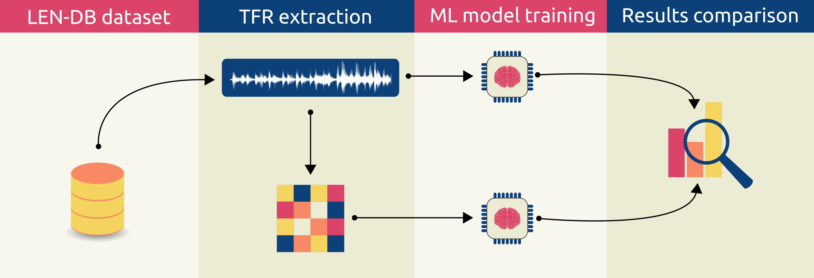
2.1. Experimental Setup

The concept of our experiment was to train three state-of-the-art CNNs using different TFRs, and compare their performance on earthquake detection with the base model. The base model was trained on the original waveform data. The experiment was divided into two parts: data preprocessing and neural network training. Data preprocessing included random sampling of the Local Earthquakes and Noise DataBase (LEN-DB) [11] (further described in Section 2.2) and TFRs extraction (further described in Section 2.3). Both the base model and the CNNs are detailed in Section 2.4. The main phases of the experiment are depicted in Figure 1.

2.2. LEN-DB Dataset

To conduct the experiment, we used the LEN-DB seismological dataset [11]. The dataset includes earthquake waveforms and noise recorded by high-gain, velocimetric seismometers from earthquakes in the magnitude range $0.4\le M\le 7.1$, originating up to 134 km from the recording stations. The data were filtered in the frequency range $0.1<f<5$ Hz. All this implies that the dataset includes very diversified trace records in terms of max amplitude and frequency content. Each instance of the dataset contains three component seismograms sampled at 20 Hz. Each seismogram contains 540 points, i.e., it is 27 s long. Illustrations of the three-component (3C) seismograms depicting an event (earthquake) and a noise instance are presented in Figure 2. The dataset contains 631,105 instances labeled as earthquakes, and 618,306 instances labeled as noise. This gives an approximate earthquake-to-noise ratio of 50:50.

In terms of uniformity, seismological data tends to have lower intra-class variance and higher inter-class variance than the, e.g., ImageNet data [12]. To clarify, in most cases, the differences between an earthquake and noise are much easier to learn and require fewer features than the differences between a tabby cat and a tiger cat (which are only two of the 1000 classes in the ImageNet dataset). Having that in mind, one can assume that even a relatively small amount of data will suffice in this experiment. Furthermore, the time required to extract TFRs and train three complex CNN models is quite significant. Consequently, we decided to use a subset of 150,000 randomly sampled three-component seismograms from the LEN-DB dataset while maintaining the original earthquake-to-noise ratio.

We split the data into training, validation, and test sets. The training set contained 104,999 instances, the validation set 22,499 instances, and the test set 22,502 instances. Each set had an approximately equal number of earthquake and noise instances, following the original ratio of the LEN-DB dataset. This waveform data were used to train the base model. The same division was maintained throughout the experiment. That means that each CNN model was trained on the same set of data as the base model, only processed by different TFRs. The same was true for the validation and the test set, so the results should reflect the effects of using TFRs with great credibility. In addition, it is worth noting that the data preprocessing procedure was parallelized due to the time-consuming nature of the process.

2.3. Extracting Time–Frequency Representations from Seismograms

Due to the oscillatory nature of seismic signals, which are non-stationary (having frequency content varying in time) and multi-component, it is necessary to develop tools to characterize and analyze them simultaneously in time and frequency. Namely, the Fourier transform provides only spectral information (information of frequencies present in the signal without their time localization). Considering the time dimension along the spectral information naturally leads to the concept of TFRs. These representations result in the 2D spreading of signal information content along the time–frequency plane.

A straightforward way to obtain signal TFR, called short-time Fourier transform (STFT), is by applying the Fourier transform to a signal windowed by a sliding window, Equation (1) [13], where x is the analyzed time-series, t denotes time, f frequency, h smoothing window (Hamming windows were used in the paper), and * denotes complex conjugate. Well-known shortcomings of the STFT are the time/frequency resolution limits caused by the fixed-sized window width. Namely, short time windows provide a better time resolution and a worse resolution in the frequency domain. On the other hand, wide windows improve frequency resolution and, at the same time, decrease the time resolution. Further, it is not possible to adjust the time and frequency resolutions independently due to a single fixed-size window (also known as Heisenberg’s uncertainty principle).

$$STF{T}_x(t,f)={\int }_{-\infty }^{+\infty }x\left(u\right)h^{*}(u-t)e^{-j2\pi fu}du$$

(1)

In many practical applications, such as seismology, instead of the STFT, the squared modulus of the STFT (known as the spectrogram, SP) is often used [13,14,15], Equation (8).

Another TFR used in this paper is Margenau–Hill (MH), defined as [16] and presented in Equation (5), where $X\left(f\right)$ stands for signal Fourier transform. In addition, the MH can also be interpreted as the real part of the product between two STFTs having different time windows. The two windows, consequently, allow for independently adjusting time and frequency resolution. The shortcoming of this approach is the possible generation of artifacts when the window lengths are significantly different, and the signal contains components with similar frequencies [17].

Another TFR was introduced by E. Wigner and further applied to the analytic signal by J. Ville. Unlike the SP where the Fourier transform was applied to a windowed signal, the Wigner–Ville distribution (WV) is performed on signal autocorrelation function resulting in quadratic TFR calculated as [18,19], Equation (10). The WV, a member of Cohen’s class of time and frequency shift-invariant TFRs, improves auto-term resolution compared to the smeared out SP; however, in the case of multi-component signals, the WV suffers from cross-terms due to its quadratic nature.

In order to reduce the cross-terms, numerous modified methods were proposed, such as windowed WV with frequency smoothing window or Pseudo WV (PWV), calculated as [20,21], Equation (6). The PWV distribution can further be modified by introducing a time-smoothing window, resulting in so-called Smoothed PWV (SPWV) defined as [20,22], Equation (9), where g stands for the time smoothing window.

Another method to reduce unwanted interferences (cross-terms) is Born–Jordan distribution (BJ), whose kernel contains the sinus cardinalis sinc, which can be viewed as the Fourier transform of the first B-Spline [23]. In particular, it damps so-called “ghost frequencies” and also effectively suppresses the noise. The BJ is expressed as [22,24], Equation (2).

Hyung-Ill Choi and William J. Williams proposed an exponential time–frequency kernel to suppress the cross-terms, which resulted in another TFR called the Choi–Williams distribution (CW), also belonging to Cohen’s class [25], Equation (4). The CW distribution does not provide an independent choice of the amount of smoothing in the time and frequency domain. Namely, its weighing function does not decay along the axis in the ambiguity domain (otherwise, it would not satisfy marginal properties), and thus, it can only filter out the cross-terms that result from the components that differ in both time and frequency center [26].

By generalizing the Choi–Williams time–frequency exponential distribution, the Butterworth distribution (BUD) was obtained [27]. Its kernel acts as a 2D filter in the ambiguity function plane with variable filter characteristics [28,29,30], Equation (3), where $\sigma$ denotes kernel width.

Finally, a reduced interference distribution based on the first kind Bessel function (RIDB) [31,32] was used in this research, Equation (7). The method is known to effectively reduce cross-terms while the auto-terms are kept due to the low-pass filter characteristics of the used Bessel kernel.

To summarize, we used the following TFRs:

• Born–Jordan (BJ) [22,24]

  $$B{J}_x(t,f)={\int }_{-\infty }^{+\infty }\frac{1}{\left|\tau \right|}{\int }_{t-\left|\tau \right|/2}^{t+\left|\tau \right|/2}x(s+\tau /2)x^{*}(s-\tau /2)ds{e}^{-j2\pi f\tau }d\tau$$

  (2)
• Butterworth (BUD) [29,32]

  $$BU{D}_x(t,f)={\int }_{-\infty }^{+\infty }\frac{\sqrt{\sigma }}{2\left|\tau \right|}{e}^{-\left|v\right|\sqrt{\sigma }\left|\tau \right|}x(t+v+\tau /2)x^{*}(t+v-\tau /2)e^{-j2\pi f\tau }dvd\tau$$

  (3)
• Choi–Williams (CW) [15,25,32]

  $$C{W}_x(t,f)=2{\int }_{-\infty }^{+\infty }{\int }_{-\infty }^{+\infty }\frac{\sqrt{\sigma }}{4\sqrt{\pi }\left|\tau \right|}{e}^{-v^2\sigma /\left(16{\tau }^2\right)}x(t+v+\tau /2)x^{*}(t+v-\tau /2)e^{-j2\pi f\tau }dvd\tau$$

  (4)
• Margenau–Hill (MH) [16]

  $$M{H}_x(t,f)=Re\left\{x\left(t\right)X\left(f\right)e^{-j2\pi ft}\right\}={\int }_{-\infty }^{\infty }\frac{1}{2}\left(x(t+\tau )x^{*}\left(t\right)+x\left(t\right)X^{*}(t-\tau )\right)e^{-j2\pi f\tau }d\tau$$

  (5)
• Pseudo Wigner–Ville (PWV) [20,21]

  $$PW{V}_x(t,f)={\int }_{-\infty }^{+\infty }h\left(\tau \right)x(t+\tau /2)x^{*}(t-\tau /2)e^{-j2\pi f\tau }d\tau$$

  (6)
• Reduced Interference Distribution with Bessel kernel (RIDB) [31,32]

  $$RID{B}_x(t,f)={\int }_{-\infty }^{+\infty }h\left(\tau \right){\int }_{t-|\tau /2|}^{t+|\tau /2|}\frac{\sqrt{2g\left(v\right)}}{\pi \left|\tau \right|}\sqrt{1-{\left(\frac{v-t}{\tau }\right)}^2}x(v+\tau /2)x^{*}(v-\tau /2)dv{e}^{-j2\pi f\tau }d\tau$$

  (7)
• Spectrogram (SP) [13,14,15]

  $$S{P}_x(t,f)=|{\int }_{-\infty }^{+\infty }x\left(u\right)h^{*}(u-t)e^{-j2\pi fu}du{|}^2$$

  (8)
• Smoothed Pseudo Wigner–Ville (SPWV) [20,22]

  $$SPW{V}_x(t,f)={\int }_{-\infty }^{+\infty }h\left(\tau \right){\int }_{-\infty }^{+\infty }g(s-t)x(s+\tau /2)x^{*}(s-\tau /2)ds{e}^{-j2\pi f\tau }d\tau$$

  (9)
• Wigner–Ville (WV) [18,19]

  $$W{V}_x(t,f)={\int }_{-\infty }^{+\infty }x(t+\tau /2)x^{*}(t-\tau /2)e^{-j2\pi f\tau }d\tau$$

  (10)

The results of the TFR extractions conducted on the LEN-DB data were three-channel, 224 × 540 images. Sample images are shown in Figure 3, Figure 4, Figure 5 and Figure 6. The heatmaps depicted in the mentioned figures indicate the presence and intensity of different frequencies in the original signal at the specific point in time. The heatmap values are TFR-dependent and do not have a specific unit of measurement. A complete list of images of all the representations is shown in Figures S1–S9. Each channel consists of 224 frequencies and 540 timeframes. TFR extraction originally produced 540 × 540 images, but we decided to logarithmically choose the first 224 frequencies, starting from the lowest one. The former was performed to reduce the size of the output data and to adapt it to the input size of the CNNs listed in Section 2.4.

As it can be noticed, some of the used TFRs may take negative values (which are, same as the interferences, the results of the mathematical transformation). This indicates that the TFRs are not energy density functions. The cause for this lies in the fact that time and frequency are non-commuting variables. Hence, it is not possible to simultaneously achieve absolute accuracy in both domains. Thus, no joint distribution (even if non-negative) may be interpreted, in a strict mathematical sense, as a probability density [33]. Nevertheless, TFRs still offer a valuable insight into the spectral nature of the signal, number of components, their time localization, and frequency modulation, to name a few.

2.4. Convnet Models and the Base Model

CNNs are a class of feed-forward neural networks whose architecture includes convolutional layers. In addition, pooling layers are also common in CNNs. CNNs are mainly used in image classification and pattern recognition due to their invariance to translation, but also, to some extent, to rotation and scale. One of the first CNNs was LeNet [34]. LeNet proved successful in identifying handwritten zip code numbers supplied by the US Postal Service.

We used three CNN architectures:

• VGG16 [35].
• AlexNet [36].
• ResNet50 [37].

Each of the listed architectures won the ImageNet classification challenge [12]. We refrained from making major modifications to the network architectures; however, we did adjust the following characteristics architecture-wise (the motivation behind this is explained in the sequel):

• Batch normalization (BN) layers were added after each convolutional layer and after each fully connected layer, except for the output layer. BN layers were not added to ResNet50 because the mentioned network originally has BN layers incorporated in its architecture.
• Inputs into the networks were adapted so that each model accepted a TFR image and three maximum channel values before data scaling. Data scaling/normalization is thoroughly described in Section 2.5.
• Outputs from the networks were adapted so that each model predicted the probability of the input data being an earthquake.

Batch normalization is a neural network training acceleration technique devised by Ioffe and Szegedy in 2015 [38]. Batch normalization layers reduce internal covariate shift allowing the training to progress at a quicker pace. Additionally, batch normalization layers have regularization effects. That is why dropout and other regularization techniques should be removed or reduced in strength when used in conjunction with BN layers.

Table 1. Original and modified regularization parameters used by the convolutional neural networks.

	L2		Dropout		Batch Normalization
	Original	Modified	Original	Modified	Original	Modified
VGG16	5$\times {10}^{-4}$	${10}^{-4}$	50%, the first two fully connected layers	✗	✗	✓
AlexNet	✗	✗	50%, the first two fully connected layers	✗	✗	✓
ResNet50	✗	✗	✗	✗	✓	✓

shows the original and modified regularization parameters used by the CNN models. The original parameters are those reported in [35,36,37], while the modified parameters are the ones used in this research. Following the practice in [38], we removed dropout and reduced L2 in strength. ResNet50 originally uses BN layers and does not employ other regularization techniques.

To utilize the full potential of BN layers, Ioffe and Szegedy recommend, among other things, to accelerate the learning rate decay and increase the learning rate. Where should BN layers be added is still a topic of debate, but the original paper states to “apply it before the nonlinearity since that is where matching the first and second moments is more likely to result in a stable distribution” [38], so we followed the same principle. Wherever we added a BN layer, we disabled the use of bias since the role of the bias is subsumed by $\beta$ in the batch normalization layer. $\beta$ is one of the parameters of a BN layer that is determined through the model training process and serves as a bias value. As it was already mentioned, training the CNN models takes quite a lot of time, so we used BN layers primarily as a means of accelerating model training.

As described in Section 2.3, the results of TFR extractions were three channel, 224 × 540 images. Each channel represents a single seismogram axis, X, Y, and Z. The chosen CNN architectures have the following input dimensions:

• VGG16—224 × 224 × 3.
• AlexNet—227 × 227 × 3.
• ResNet50—224 × 224 × 3.

It is obvious that some sort of input adaptation was necessary. For VGG16 and ResNet50, we added two max pooling layers before the original input layer. The first max pooling layer had both a size, (height, width), and a stride of (1, 2), while the second pooling layer had a size of (1, 47) and a stride of (1, 1). AlexNet’s input size differs from the formerly mentioned CNNs, so a slightly different scheme was applied there. Firstly, a zero padding layer was added, having a dimension of (3, 0). Because the time component of a TFR image is large enough, only the frequency component needs to be padded. The zero padding layer produces 230 × 540 × 3 images, which are then fed to the two max pooling layers. The first one has a size and a stride of (1, 2), while the second one has a size of (4, 44) and a stride of (1, 1). By applying the described scheme, we believe to have adapted the input layers of the networks while minimizing the modifications of the original architectures.

The three used CNN architectures have 1000 neurons in their output layers. This stems from the fact that the architectures were originally devised for dealing with the ImageNet [12] dataset, which contains 1000 classes. Because we are interested in classifying whether something is or is not an earthquake, we only need one sigmoid neuron in the output layer. In addition, because we believed that the maximum values of each of the three channels (before data scaling) would enhance classification performance, along with modifying the output layers to have a single sigmoid neuron, we also added channel max data input as close to the output layer as possible. The same was performed in [5]. Jozinović et al. showed that this procedure is highly effective [39]. In VGG16 and AlexNet, max channel data were concatenated with the last fully connected layer before the output neuron. In ResNet50, channel max data were concatenated with the global average pooling layer. All the described modifications resulted in CNNs that are capable of accepting 224 × 540 × 3 TFR input along with three channel max values before data scaling, and are capable of outputting the probability that the input data represents an earthquake. Each CNN model takes approximately 24 h to train.

We also trained the base model as a means of comparing classification accuracy with the CNNs trained on TFR representations. We chose the model described in [4]. The original model accepts three-channel waveform data of size $1000\times 3$. As described in Section 2.2, LEN-DB waveform data have three channels, each consisting of 540 samples. To match LEN-DB data size with the model input, we padded waveform data with 230 zeros on each side. Further, as formerly described, maximum channel values before scaling were added to the last fully connected layer. The output layer was also adapted to enable earthquake classification. No other modifications were made to the base model. We retained L2 regularization with $\lambda =0.001$. The base model, being much simpler than the CNN models, takes about 1 h to train; therefore, BN layers were not added to the architecture and the original regularization procedure was retained. It is important to emphasize that we normalized the inputs into neural networks, both in case of CNN models and the base model. Input normalization is described in Section 2.5.

Since our primary concern is the usefulness of TFRs, the single important thing when choosing the models is that they have sufficient capacity. Neural network capacity can “be viewed as an upper bound on the number of bits that can be stored in the architecture during learning, or equivalently an upper bound on the number of bits that can be extracted from the training data” [40]. It is clear that the capacity of a neural network should be assessed with respect to the complexity of the problem the network is expected to solve. Consequently, the neural network of insufficient capacity is guaranteed to underfit. Given the fact that the used CNN architectures were originally designed to deal with the ImageNet dataset [12], which is a multi-class high-variance dataset, we are confident that all the architectures have sufficient capacity in the context of this experiment. To make the comparisons as unbiased as possible, we tried to use the original hyperparameter values and refrained from making any major modifications to the networks. This was described earlier in this subsection.

Table 2. Training parameters that were used for the experiment.

	Optimizer	Learning Rate	Decay	Momentum	Batch Size	Epochs
CNN (all TFRs except spectrogram)	SGD	0.1	0.0001	0.9	16	30
CNN (spectrogram)	SGD	0.0001	0.0001	0.9	16	30
Base model	Adam	0.0001	✗	✗	128	500

lists the training parameters that were used. For CNNs, we mostly relied on ResNet50 training parameters due to the fact that it originally uses BN layers in its architecture.

However, while conducting the experiment, we noticed that the spectrogram TFR was underperforming. The results achieved on the validation dataset by all three CNNs were a clear indicator of an overly large learning rate; therefore, we assessed the performance with many different learning rates ranging from 0.01 to 0.00001. The learning rate of 0.0001 was the first to yield significant improvements, while 0.00001 achieved the same results as 0.0001, but had longer training time, which was expected. The tested learning rates had no positive or negative effects when applied to other TFRs. The only difference was the extended training time. Due to that, we decided to apply the learning rate of 0.0001 when CNNs were trained on spectrogram data, and a learning rate of 0.1 when we used other TFRs. Each CNN model was trained for a maximum of 30 epochs. The learning rate was divided by 10 if there was no improvement in validation loss over 5 consecutive epochs. Similarly, the training was stopped if there was no improvement in validation loss over 10 consecutive epochs.

2.5. Input Normalization

Input normalization brings specific benefits into neural network training [41,42]. More specifically, data normalization brings different features into the similar value range, and therefore facilitates the gradient flow during neural network training, consequently yielding a model with superior performance. We normalized the data by scaling each channel separately, i.e., by determining the minimum and maximum values and applying the following expression:

$$\eta =\frac{\gamma -\beta }{\alpha -\beta },$$

(11)

where $\eta$ represents the value after scaling, $\alpha$ is the maximum channel value, $\beta$ is the minimum channel value, and $\gamma$ is the value that needs to be scaled. This brought each value of each channel in the range between zero and one, inclusive. Further, we saved maximum values of each channel for each instance and used them in neural network training.

Furthermore, we calculated a per-channel mean image (i.e., a three-channel mask) on the training set for each TFR separately. The mask is of the same shape as TFR images and contains average values of each pixel, i.e., each pixel of each channel is a separate feature. Let M be a zero tensor of dimension $224\times 540\times 3$. Let T be a 4-D tensor containing TFR training set images. T’s shape is $N\times 224\times 540\times 3$, where N represents the number of images in the training set. Equation (12) describes how mask calculation is conducted for each element of the mask tensor. The mask was then applied to the validation set and the test set.

$$M_{ijk}=\frac{{\sum }_{m=1}^N{T}_{mijk}}{N}$$

(12)

The same normalization procedure we applied to the TFR data was also applied to the original waveform data that were used for the base model training. We scaled each channel separately by using Equation (11). As described in Section 2.2, waveform data dimensions are $540\times 3$. Hence, when calculating the mask, each value of each channel represents a separate feature. Equation (12) can therefore be adapted to allow for the smaller number of dimensions when dealing with waveform data. Let M be a zero tensor of dimension $540\times 3$. Let T be a 3-D tensor containing training set waveform data. T’s shape is $N\times 540\times 3$, where N represents the number of instances in the training set. Equation (13) describes how mask calculation is conducted for each element of the mask tensor.

$$M_{ij}=\frac{{\sum }_{m=1}^N{T}_{mij}}{N}$$

(13)

2.6. Evaluation Metrics

We evaluated the results based on three indicators: receiver operating characteristic (ROC) curve, area under the ROC curve (AUC), and classification accuracy. A model is evaluated using different probability thresholds. Obtained true positive rates (TPRs) and false positive rates (FPRs) show the level of certainty the model has while classifying the data. TPRs and FPRs can be plotted one against another, and the AUC can be calculated. The ideal AUC value is 1, but in practice, it is fairly hard to achieve it. We also tested the classification accuracies of our models by applying the standard threshold of 0.5. The following equation demonstrates the rounding rule that we used:

$$f\left(x\right)=\left\{\begin{array}{cc}1\hfill & x\in [0.5,1]\hfill \\ 0\hfill & x\in [0,0.5)\hfill \end{array}\right.,$$

(14)

where x represents the model’s prediction, while $f\left(x\right)$ represents the output class—earthquake (1) or noise (0).

2.7. Statistical Significance

A series of statistical tests were performed to determine if the results are strong enough to draw solid conclusions about the usefulness of TFRs. We used McNemar’s test because “for algorithms that can be executed only once, McNemar’s test is the only test with acceptable Type I error” [43]. Our goal was to assess if any of the used TFRs enhances original data and, as a consequence, yields models whose performance significantly surpasses the performance of the base model. The idea was to keep the significance level $\alpha$ at 0.01 for each TFR. Due to the fact that each TFR was applied to three different CNN architectures, we utilized the Bonferroni correction [44] and divided $\alpha$ by 3. This resulted in significance level $\alpha =0.00\overline{3}$ for each TFR–CNN couple. Each comparison was made between the results of a CNN coupled with a TFR and the results of the base model.

3. Results

The final results on the test dataset are presented in

Table 3. The results of model evaluation using classification accuracy measured on the test dataset. Each time–frequency representation is coupled with a convolutional neural network. The best performing combination is marked in green, while the worst performing one is marked in red. The results of the base model are marked in gray.

Time–Frequency Representation	CNN Architecture
	VGG16	ResNet50	AlexNet
BJ	94.69%	94.52%	94.28%
BUD	93.86%	93.39%	92.41%
CW	92.68%	93.03%	93.75%
MH	86.45%	88.70%	88.79%
PWV	95.11%	95.57%	95.71%
RIDB	94.94%	95.00%	94.47%
SP	92.46%	93.74%	92.55%
SPWV	93.21%	93.79%	90.34%
WV	94.90%	95.24%	94.72%
Base	94.15%

and

Table 4. The results of model evaluation using the area under the receiver operating characteristic curve measured on the test dataset. Each time–frequency representation is coupled with a convolutional neural network. The best performing combination is marked in green, while the worst performing one is marked in red. The results of the base model are marked in gray.

Time–Frequency Representation	CNN Architecture
	VGG16	ResNet50	AlexNet
BJ	0.9807	0.9791	0.9762
BUD	0.9725	0.9697	0.9608
CW	0.967	0.9697	0.9706
MH	0.9253	0.9484	0.9509
PWV	0.9826	0.9857	0.9859
RIDB	0.9811	0.9815	0.9783
SP	0.962	0.9715	0.9618
SPWV	0.9679	0.9677	0.9415
WV	0.9824	0.9841	0.9805
Base	0.9785

. Table 3 lists the final accuracies on the test set, while Table 4 lists the AUC values. Base model results are marked in gray, the best TFR–model combination in green, and the worst TFR–model combination in red. Additional results are presented in Figure S10, where each subfigure represents the base model and all the TFRs coupled with a specific CNN. Figures S11–S19 focus on the base model results and how they compare to the TFRs.

The base model achieved an accuracy of 94.15% and an AUC of 0.9785. The best TFR results were achieved by AlexNet architecture combined with Pseudo Wigner–Ville TFR. The mentioned combination achieved an accuracy of 95.71% and an AUC of 0.9859. On the other hand, the worst performing combination was the one between VGG16 and Margenau–Hill TFR, which achieved an accuracy of 86.45% and an AUC of 0.9253.

Table 5. p-values of the performed statistical tests ($\alpha =0.00\overline{3}$), using McNemar’s test. Each time–frequency representation is coupled with a convolutional neural network. The values are rounded to three decimal places. Statistically significant cases are marked in green and red. Green is used to indicate that a time–frequency representation model performed better than the base model, while red is used to emphasize the opposite. The cases where no statistically significant differences between the results of a time–frequency representation model and the base model were observed are marked in gray.

Time–Frequency Representation	CNN Architecture
	VGG16	ResNet50	AlexNet
BJ	0	0.01	0.323
BUD	0.042	0	0
CW	0	0	0.007
MH	0	0	0
PWV	0	0	0
RIDB	0	0	0.016
SP	0	0.002	0
SPWV	0	0.014	0
WV	0	0	0

lists p-values for all the comparisons. We used McNemar’s test [43]. We should note that the p-values were rounded to three decimal places. Statistically significant cases are marked in green and red. Green is used to indicate that a TFR model performed better than the base model, while red is used to emphasize the opposite. The cases where no statistically significant differences between the results of a time–frequency representation model and the base model were observed are marked in gray.

4. Discussion

This research shows that the most common TFR traditionally used in seismology, the spectrogram, has better performing alternatives. Because we used fairly complex CNNs and a well-determined training protocol, a reasonable assumption is that both the CNNs and the base model had an equal opportunity to learn the differences between earthquake and noise seismograms; therefore, the key factor preventing CNN results from being significantly better than those of the base model are the data representations that were used to train the CNN models. Further to the previous point, if a TFR yields significantly better results than the base model when coupled with all three CNNs, we conclude that the particular TFR significantly enhances waveform data and, also, gives superior accuracy. The opposite is also true. In addition, if a row connected to a certain TFR (see Table 5) contains even a single result that is not statistically significant, we can not draw a conclusion about that particular TFR. The same is true if a single row contains cells that contradict each other, i.e., the p-values infer TFR superiority and inferiority at the same time. Given the p-values presented in Table 5, and the statistical significance level of $\alpha =0.00\overline{3}$, we can conclude that Pseudo Wigner–Ville and Wigner–Ville TFRs significantly enhance waveform data, while Margenau–Hill and spectrogram TFRs significantly worsen the results. We can not claim anything about the remaining five TFRs, that is, the remaining TFRs are as informative as the original data. The conclusions are based on the randomly sampled subset of the LEN-DB dataset that was used in the experiment.

Pseudo Wigner–Ville TFR coupled with AlexNet CNN achieves 1.56 percentage points better results than the base model, while Wigner–Ville TFR coupled with ResNet50 CNN surpasses the base model by 1.09 percentage points. The increase in accuracy is important as the waveforms misclassified in the original study, [11], mainly come from the stations that have high noise levels. This suggests that the selection of a TFR helps the machine learning model to achieve significant improvements on those stations. The former could be of crucial importance for the applications of machine learning in seismology on sensors featuring higher instrumental noise. Consequently, researchers will have higher quality data to further study earthquake occurrence and phenomena linked to it.

Because the difference in performance between the base and the TFR models is quite close, we used a McNemar’s test of statistical significance. The test does not directly compare model accuracies, but focuses on the cases where the base model and the TFR model disagreed in predictions. It then checks if there is a statistically significant difference in their performance. In the context of our experiment, we can say it is highly unlikely the results presented in the tables arose by chance, if there is no statistically significant difference between machine learning model performance on raw waveform data and on the TFRs.

Perhaps the most important result is that by applying the PWV or WV TFRs to the recorded data, seismologists can exploit the data better to lower the magnitude of the earthquake detection level. This indeed, because of the magnitude–occurrence Gutenberg–Richter law, can result in a large increase in earthquakes in the catalogs and, to some extent, reduce the need to add new stations with an overall reduction in the costs.

An interesting observation is that the spectrogram TFR, which is often used in non-stationary signal analysis, performed significantly worse than the original waveform data. Seeing that the results achieved using TFRs suggest their usefulness in machine learning modeling, we believe that TFRs could prove useful in other domains as well, e.g., EEG and ECG signals, gravitational waves, speech data, and so on; however, this should be further inspected.

Since the LEN-DB dataset contains an approximately equal number of earthquake and noise instances, the work presented in the paper does not take into account possible class imbalance; however, the proposed methodology could easily be adapted to investigate such a scenario. The only necessary modification of the experiment workflow is the use of evaluation metrics appropriate for imbalanced datasets, such as Matthews correlation coefficient, precision–recall curve, F1 score, etc.

We should note that, in addition to the LEN-DB dataset, we also considered other datasets for this research, such as STanford EArthquake Dataset (STEAD) [45]; however, given the complexity and the time-consuming nature of extracting TFRs, along with the time needed to train three intricate CNN models using nine TFRs, we decided to limit the experiment to the LEN-DB dataset only as it had the waveforms with the smallest size between the considered datasets. As our hypothesis is that TFRs might affect the classification accuracies of machine learning models, a confirmation of the hypothesis on a single dataset presents sufficient evidence for its approval, which mitigates the necessity to use other datasets.

Inclusion of spatio-temporal information proved as a viable way to enhance deep learning models [46,47,48], and has been performed in seismic applications of machine learning mainly by using multi-station input data (e.g., [49,50]). Such applications could perhaps also be improved by using the alternative TFRs suggested here (it, however, needs to be tested). Additionally, our analysis could be easily expanded by, e.g., incorporating magnitude prediction in the experiment (similar as in our recent paper on examining transfer learning between different domains [51]). This is, however, out of the scope of this study.

5. Conclusions

Building on top of [4,5], this research explored the possibility of TFRs being more informative than raw waveform data or commonly used spectrograms for non-stationary signals analysis. More specifically, we tested the effects of TFRs on machine learning classification. The data used in the experiment were a subset of LEN-DB seismological dataset [11]. We used nine TFRs coupled with three respectable CNNs.

The results show that a number of combinations surpasses the accuracy of the base model described in [4]. In addition, tests of statistical significance suggest that Pseudo Wigner–Ville and Wigner–Ville TFRs significantly enhance waveform representations and result in higher classification accuracies, while Margenau–Hill and spectrogram TFRs worsen the results (p < 0.01). The best combination, the one between AlexNet architecture and Pseudo Wigner–Ville TFR, achieves 1.56 percentage points better accuracy than the base model.

Given the vast amount of earthquakes that happen every year, this results in a significant increase in the number of correctly classified events. Moreover, the analysis of the results suggests that the phenomena that were previously hidden in the seismic noise are now more easily identified; however, the main conclusion of the paper is that the machine learning model accuracy is significantly affected by the representation of the input data. More precisely, we show that Pseudo Wigner–Ville TFR improves the performance of the machine learning models (AlexNet, ResNet50, VGG16) for earthquake detection the most, both in terms of classification accuracy and AUC. In addition, the results indicate the possibility of alternative TFRs extracting more useful information from the original data, which may be applicable in various other fields that deal with non-stationary signals. This is a promising indicator that opens ways to new research opportunities.

References

1. Withers, M.; Aster, R.; Young, C.; Beiriger, J.; Harris, M.; Moore, S.; Trujillo, J. A comparison of select trigger algorithms for automated global seismic phase and event detection. Bull. Seismol. Soc. Am. 1998, 88, 95–106. [Google Scholar] [CrossRef]
2. Yoon, C.E.; O’Reilly, O.; Bergen, K.J.; Beroza, G.C. Earthquake detection through computationally efficient similarity search. Sci. Adv. 2015, 1, e1501057. [Google Scholar] [CrossRef] [PubMed] [Green Version]
3. Rojas, O.; Otero, B.; Alvarado, L.; Mus, S.; Tous, R. Artificial neural networks as emerging tools for earthquake detection. Comput. Sist. 2019, 23, 350. [Google Scholar] [CrossRef]
4. Perol, T.; Gharbi, M.; Denolle, M. Convolutional neural network for earthquake detection and location. Sci. Adv. 2018, 4, e1700578. [Google Scholar] [CrossRef] [PubMed] [Green Version]
5. Lomax, A.; Michelini, A.; Jozinović, D. An Investigation of Rapid Earthquake Characterization Using Single-Station Waveforms and a Convolutional Neural Network. Seismol. Res. Lett. 2019, 90, 517–529. [Google Scholar] [CrossRef]
6. Zhou, Y.; Yue, H.; Kong, Q.; Zhou, S. Hybrid Event Detection and Phase-Picking Algorithm Using Convolutional and Recurrent Neural Networks. Seismol. Res. Lett. 2019, 90, 1079–1087. [Google Scholar] [CrossRef]
7. Tous, R.; Alvarado, L.; Otero, B.; Cruz, L.; Rojas, O. Deep Neural Networks for Earthquake Detection and Source Region Estimation in North-Central Venezuela. Bull. Seismol. Soc. Am. 2020, 110, 2519–2529. [Google Scholar] [CrossRef]
8. Mousavi, S.M.; Zhu, W.; Sheng, Y.; Beroza, G.C. CRED: A Deep Residual Network of Convolutional and Recurrent Units for Earthquake Signal Detection. Sci. Rep. 2019, 9, 10267. [Google Scholar] [CrossRef]
9. Dokht, R.M.; Kao, H.; Visser, R.; Smith, B. Seismic event and phase detection using time-frequency representation and convolutional neural networks. Seismol. Res. Lett. 2019, 90, 481–490. [Google Scholar] [CrossRef]
10. Mousavi, S.M.; Langston, C.A. Fast and novel microseismic detection using time-frequency analysis. In SEG Technical Program Expanded Abstracts; Society of Exploration Geophysicists: Tulsa, OK, USA, 2016; Volume 35. [Google Scholar] [CrossRef]
11. Magrini, F.; Jozinović, D.; Cammarano, F.; Michelini, A.; Boschi, L. Local earthquakes detection: A benchmark dataset of 3-component seismograms built on a global scale. Artif. Intell. Geosci. 2020, 1, 1–10. [Google Scholar] [CrossRef]
12. Russakovsky, O.; Deng, J.; Su, H.; Krause, J.; Satheesh, S.; Ma, S.; Huang, Z.; Karpathy, A.; Khosla, A.; Bernstein, M.; et al. ImageNet Large Scale Visual Recognition Challenge. Int. J. Comput. Vis. 2015, 115, 211–252. [Google Scholar] [CrossRef] [Green Version]
13. Ackroyd, M.H. Short-time spectra and time-frequency energy distributions. J. Acoust. Soc. Am. 1971, 50, 1229–1231. [Google Scholar] [CrossRef]
14. Flandrin, P. Time-Frequency/Time-Scale Analysis; Academic Press: Cambridge, MA, USA, 1998. [Google Scholar]
15. Hlawatsch, F.; Auger, F. Time-Frequency Analysis; John Wiley & Sons: Hoboken, NJ, USA, 2013. [Google Scholar]
16. Margenau, H.; Hill, R.N. Correlation between Measurements in Quantum Theory. Prog. Theor. Phys. 1961, 26, 722–738. [Google Scholar] [CrossRef] [Green Version]
17. Volpato, A.; Collini, E. Time-frequency methods for coherent spectroscopy. Opt. Express 2015, 23, 20040. [Google Scholar] [CrossRef]
18. Ville, J. Theorie et application dela notion de signal analytique. Câbles Transm. 1948, 2, 61–74. [Google Scholar]
19. Boashash, B. Time-Frequency Signal Analysis and Processing: A Comprehensive Reference; Academic Press: Cambridge, MA, USA, 2015. [Google Scholar]
20. Claasen, T.; Mecklenbräuker, W. The Wigner distribution—A tool for time-frequency signal analysis, Parts I–III. Philips J. Res. 1980, 35, 217–250, 276–300, 372–389. [Google Scholar]
21. Flandrin, P.; Escudié, B. An interpretation of the pseudo-Wigner-Ville distribution. Signal Process. 1984, 6, 27–36. [Google Scholar] [CrossRef]
22. Flandrin, P. Some features of time-frequency representations of multicomponent signals. In Proceedings of the IEEE International Conference on Acoustics, Speech, and Signal Processing (ICASSP ’84), Institute of Electrical and Electronics Engineers, San Diego, CA, USA, 19–21 March 1984; Volume 9, pp. 266–269. [Google Scholar] [CrossRef]
23. Cordero, E.; de Gosson, M.; Dörfler, M.; Nicola, F. Generalized Born-Jordan distributions and applications. Adv. Comput. Math. 2020, 46, 51. [Google Scholar] [CrossRef]
24. Jeong, J.; Williams, W.J. Kernel design for reduced interference distributions. IEEE Trans. Signal Process. 1992, 40, 402–412. [Google Scholar] [CrossRef]
25. Choi, H.I.; Williams, W.J. Improved Time-Frequency Representation of Multicomponent Signals Using Exponential Kernels. IEEE Trans. Acoust. Speech Signal Process. 1989, 37, 862–871. [Google Scholar] [CrossRef]
26. Hlawatsch, F.; Manickam, T.G.; Urbanke, R.L.; Jones, W. Smoothed pseudo-Wigner distribution, Choi-Williams distribution, and cone-kernel representation: Ambiguity-domain analysis and experimental comparison. Signal Process. 1995, 43, 149–168. [Google Scholar] [CrossRef]
27. Papandreou, A.; Boudreaux-Bartels, G.F. Distributions for time-frequency analysis: A generalization of Choi-Williams and the Butterworth distribution. In Proceedings of the 1992 IEEE International Conference on Acoustics, Speech, and Signal Processing (ICASSP-92), San Francisco, CA, USA, 23–26 March 1992; Volume 5, pp. 181–184. [Google Scholar] [CrossRef]
28. Wu, D.; Morris, J.M. Time-frequency representations using a radial Butterworth kernel. In Proceedings of the IEEE-SP International Symposium on Time- Frequency and Time-Scale Analysis, Philadelphia, PA, USA, 25–28 October 1994; pp. 60–63. [Google Scholar] [CrossRef]
29. Papandreou, A.; Boudreaux-Bertels, G. Generalization of the Choi-Williams Distribution and the Butterworth Distribution for Time-Frequency Analysis. IEEE Trans. Signal Process. 1993, 41, 463. [Google Scholar] [CrossRef]
30. Auger, F. Représentations Temps-Fréquence des Signaux Non-Stationnaires: Synthèse et Contribution. Ph.D. Thesis, Ecole Centrale de Nantes, Nantes, France, 1991. [Google Scholar]
31. Guo, Z.; Durand, L.G.; Lee, H. The time-frequency distributions of nonstationary signals based on a Bessel kernel. IEEE Trans. Signal Process. 1994, 42, 1700–1707. [Google Scholar] [CrossRef]
32. Auger, F.; Flandrin, P.; Goncalves, P.; Lemoine, O. Time-Frequency Toolbox Reference Guide. Hewston Rice Univ. 2005, 180, 1–179. [Google Scholar]
33. Man’ko, V.I.; Mendes, R.V. Non-commutative time-frequency tomography. Phys. Lett. Sect. A Gen. At. Solid State Phys. 1999, 263. [Google Scholar] [CrossRef] [Green Version]
34. Lecun, Y.; Bottou, L.; Bengio, Y.; Haffner, P. Gradient-based learning applied to document recognition. Proc. IEEE 1998, 86, 2278–2324. [Google Scholar] [CrossRef] [Green Version]
35. Simonyan, K.; Zisserman, A. Very deep convolutional networks for large-scale image recognition. arXiv 2015, arXiv:1409.1556v6. [Google Scholar]
36. Krizhevsky, A.; Sutskever, I.; Hinton, G.E. ImageNet classification with deep convolutional neural networks. Commun. ACM 2017, 60, 84–90. [Google Scholar] [CrossRef]
37. He, K.; Zhang, X.; Ren, S.; Sun, J. Deep residual learning for image recognition. In Proceedings of the 2016 IEEE Conference on Computer Vision and Pattern Recognition (CVPR), Las Vegas, NV, USA, 27–30 June 2016; pp. 770–778. [Google Scholar]
38. Ioffe, S.; Szegedy, C. Batch normalization: Accelerating deep network training by reducing internal covariate shift. arXiv 2015, arXiv:1502.03167. [Google Scholar]
39. Jozinović, D.; Lomax, A.; Štajduhar, I.; Michelini, A. Rapid prediction of earthquake ground shaking intensity using raw waveform data and a convolutional neural network. Geophys. J. Int. 2020, 222, 1379–1389. [Google Scholar] [CrossRef]
40. Baldi, P.; Vershynin, R. The capacity of feedforward neural networks. Neural Netw. 2019, 116, 288–311. [Google Scholar] [CrossRef] [Green Version]
41. Nawi, N.M.; Atomi, W.H.; Rehman, M. The Effect of Data Pre-processing on Optimized Training of Artificial Neural Networks. Procedia Technol. 2013, 11, 32–39. [Google Scholar] [CrossRef] [Green Version]
42. Singh, D.; Singh, B. Investigating the impact of data normalization on classification performance. Appl. Soft Comput. 2020, 97, 105524. [Google Scholar] [CrossRef]
43. Dietterich, T.G. Approximate Statistical Tests for Comparing Supervised Classification Learning Algorithms. Neural Comput. 1998, 10, 1895–1923. [Google Scholar] [CrossRef] [Green Version]
44. Bonferroni, C.E. Teoria statistica delle classi e calcolo delle probabilità. Pubbl. R Ist. Sup. Sci. Econ. Commer. Fir. 1936, 8, 3–62. [Google Scholar]
45. Mousavi, S.M.; Sheng, Y.; Zhu, W.; Beroza, G.C. STanford EArthquake Dataset (STEAD): A Global Data Set of Seismic Signals for AI. IEEE Access 2019, 7, 179464–179476. [Google Scholar] [CrossRef]
46. Amato, F.; Guignard, F.; Robert, S.; Kanevski, M. A novel framework for spatio-temporal prediction of environmental data using deep learning. Sci. Rep. 2020, 10, 22243. [Google Scholar] [CrossRef]
47. Wang, S.; Cao, J.; Yu, P. Deep Learning for Spatio-Temporal Data Mining: A Survey. IEEE Trans. Knowl. Data Eng. 2020, 1. [Google Scholar] [CrossRef]
48. Wang, L.; Xu, T.; Stoecker, T.; Stoecker, H.; Jiang, Y.; Zhou, K. Machine learning spatio-temporal epidemiological model to evaluate Germany-county-level COVID-19 risk. Mach. Learn. Sci. Technol. 2021, 2, 035031. [Google Scholar] [CrossRef]
49. Kriegerowski, M.; Petersen, G.M.; Vasyura-Bathke, H.; Ohrnberger, M. A deep convolutional neural network for localization of clustered earthquakes based on multistation full waveforms. Seismol. Res. Lett. 2019, 90, 510–516. [Google Scholar] [CrossRef]
50. Jozinović, D.; Lomax, A.; Štajduhar, I.; Michelini, A. Transfer learning: Improving neural network based prediction of earthquake ground shaking for an area with insufficient training data. Geophys. J. Int. 2022, 229, 704–718. [Google Scholar] [CrossRef]
51. Otović, E.; Njirjak, M.; Jozinović, D.; Mauša, G.; Michelini, A.; Štajduhar, I. Intra-domain and cross-domain transfer learning for time series data—How transferable are the features? Knowl.-Based Syst. 2022, 239, 107976. [Google Scholar] [CrossRef]
Figure 1. A diagram depicting the main phases of the experiment.
Mathematics 10 00965 g001
Figure 2. Two randomly sampled seismogram instances from the LEN-DB dataset, depicting (a) an event (earthquake) and (b) noise.
Mathematics 10 00965 g002
Figure 3. Pseudo Wigner–Ville transformations of (a) an earthquake and (b) noise shown in Figure 2. All three axes are presented.
Mathematics 10 00965 g003
Figure 4. Wigner–Ville transformations of (a) an earthquake and (b) noise shown in Figure 2. All three axes are presented.
Mathematics 10 00965 g004
Figure 5. Margenau–Hill transformations of (a) an earthquake and (b) noise shown in Figure 2. All three axes are presented.
Mathematics 10 00965 g005
Figure 6. Spectrogram transformations of (a) an earthquake and (b) noise shown in Figure 2. All three axes are presented.
Mathematics 10 00965 g006