Modified Projection Method with Inertial Technique and Hybrid Stepsize for the Split Feasibility Problem

Abstract

We designed a modified projection method with a new condition of the inertial step and the step size for the split feasibility problem in Hilbert spaces. We show that our iterate weakly converged to a solution. Lastly, we give numerical examples and comparisons that could be applied to signal recovery to show the efficiency of our method.

1. Introduction

The convex feasibility problem (CFP) is to find a feasible point in the intersection of finitely many convex and closed sets. The CFP formalism is at the core of the modeling of many inverse problems in various areas of mathematics. The split equality problem (SFP) is a classical inverse problem that is formulated as follows [1]:

$$\begin{array}{c}\hfill \mathrm{finding}s\in C,t\in Q\mathrm{such}\mathrm{that}As=Bt,\end{array}$$

(1)

where $C\subset {\mathbb{R}}^K$, $Q\subset {\mathbb{R}}^P$, are nonempty closed convex sets. A and B are $M\times K$ and $M\times P$ real matrices, respectively, and $M,K,P$ are positive integers. See also [1,2,3,4].

Now, we consider the split feasibility problem (SFP) that was proposed by Censor and Elfving [5] and is formulated as

$$\begin{array}{c}\hfill \mathrm{finding}{s}^{*}\in C\mathrm{such}\mathrm{that}A{s}^{*}\in Q,\end{array}$$

(2)

where $A:X\to Y$ is a bounded linear operator, C and Q are nonempty closed and convex subsets of real Hilbert spaces X and Y, respectively. SEP is an extension of SFP.

SFP can be applied to real-world problems such as image processing, signal recovery, and data classification; see [5,6,7,8,9,10]. There are many methods for solving the split feasibility problem [11,12,13,14,15,16,17,18]. One of the most popular is the CQ method of Byrne [19]. In 2004, Yang [20] introduced the relaxed CQ method onto half space. For these methods, step sizes are based on the norm operator and are generally not easy to compute.

Afterwards, line-search step sizes that do not depend on norm operator were introduced. In 2012, Zhao et al. [21] introduced the modified projection method for SFP. In 2018, Gibali et al. [22] proposed the modified relaxation CQ algorithm for split feasibility with the Armijo line search. In 2012, López et al. [23] suggested the stepsizes that do not require the prior knowledge of matrix norms for SFP.

In addition, to speed up the convergence, the methods were also improved by adding an inertial step in iterative, see Nesterov [24]. In 2020, Shehu and Gibali [25] introduced a relaxed CQ method with alternated inertial step for SFP.

The purpose of this work is to design a new projection method by using the inertial step and the stepsize defined by López et al. [23] for solving SFP. We prove the weak convergence of our iterations. To show its efficiency, we present a comparison with algorithm of Gibali et al. [22] and algorithm of Shehu and Gibali [25] in signal recovery.

The paper is organized as follows. Section 2 presents preliminaries and lemmas that are used throughout the paper. In Section 3, we describe our new relaxed CQ algorithm with inertial step and prove the weak convergence theorem. In Section 4, we apply the proposed algorithm to signal recovery and give a comparison to algorithm of Gibali et al. [22] and algorithm of Shehu and Gibali [25]. Lastly, conclusions are given in Section 5.

2. Preliminaries and Lemmas

We now give some preliminaries and mathematical tools for proving our convergence theorem. Symbol ⇀ stands for weak convergence. Mapping $T:X\to X$ is

• firmly nonexpansive if

  $$\langle Ts-Tt,s-t\rangle \ge {\parallel Ts-Tt\parallel }^2,\mathrm{for}\mathrm{all}s,t\in X.$$

  (3)
• g is convex if and only if:

  $$g(w)\ge g(s)+\langle \nabla g(s),w-s\rangle ,\mathrm{for}\mathrm{all}w\in X.$$

  (4)

Lemma 1

([26]). Let X be a real Hilbert space, and let C be a nonempty closed convex subset of a real Hilbert space X; we have

(1) 

$\langle s-P_{C}s,w-P_{C}s\rangle \le 0$ for all $w\in C$;

(2) 

$\parallel P_{C}s-P_C{t\parallel }^2\le \langle P_{C}s-P_{C}t,s-t\rangle$ for all $s,t\in X$;

(3) 

$\parallel P_C{s-w\parallel }^2\le {\parallel s-w\parallel }^2-{\parallel P_{C}s-s\parallel }^2$ for all $w\in C$.

Lemma 2

([27]). Let $\left\{a_k\right\}$, $\left\{b_k\right\}$ and $\left\{c_k\right\}$ be positive sequences, such that

$$\begin{array}{c}\hfill a_{k+1}\le (1+c_k)a_k+b_k,k\ge 1.\end{array}$$

If ${\sum }_{k=1}^{\infty }{c}_k<+\infty$ and ${\sum }_{k=1}^{\infty }{b}_k<+\infty$; then, ${\displaystyle \underset{k\to +\infty }{lim}{a}_k}$ exists.

Lemma 3

([28]). Let $\left\{a_k\right\}$ and $\left\{{\beta }_k\right\}$ be positive sequences, such that

$$\begin{array}{c}\hfill a_{k+1}\le (1+{\beta }_k)a_k+{\beta }_k{a}_{k-1},k\ge 1.\end{array}$$

Then, $a_{k+1}\le N·{\prod }_{i=1}^k(1+2{\beta }_i)$ where $N=max\{a_1,a_2\}.$ Moreover, if ${\sum }_{k=1}^{\infty }{\beta }_k<+\infty$; then, $\left\{a_k\right\}$ is bounded.

Lemma 4

([29]). Let X be a real Hilbert space, and let Ω be a nonempty subset of a real Hilbert space X. Assume that $\left\{s_k\right\}$ is a sequence in X, such that

(i) 

${\displaystyle \underset{k\to \infty }{lim}\parallel s_k-s\parallel }$ exists for each $s\in \mathsf{\Omega }$;

(ii) 

every sequential weak limit point of $\left\{s_k\right\}$ is in Ω.

Then $\left\{s_k\right\}$ converges weakly to a point in Ω.

3. Main Results

Next, we propose a new relaxed CQ algorithm with inertial step and prove the weak convergence theorem. Let $\mathsf{\Omega }$ be the set of solutions of SFP. Define sets $C_k$ and $Q_k$ by

$$\begin{array}{c}\hfill C_k=\{s\in X:c(s_k)\le \langle {\eta }_k,s_k-s\rangle \},\end{array}$$

(5)

where ${\eta }_k\in \mathsf{\partial }c(s_k)$ and $c:X\to \mathbb{R}$ are convex functions,

$$\begin{array}{c}\hfill Q_k=\{t\in Y:q(A{s}_k)\le \langle {\phi }_k,A{s}_k-t\rangle \},\end{array}$$

(6)

where ${\phi }_k\in \mathsf{\partial }q(A{s}_k)$ and $q:Y\to \mathbb{R}$ are convex functions.

Since c and q are subdifferentiable on C and Q, respectively, c and q are bounded on bounded sets.

Set

$$\begin{array}{c}\hfill {\displaystyle g_k(s)=\frac{1}{2}{\parallel (I-P_{Q_k})As\parallel }^2,k\ge 1.}\end{array}$$

(7)

We then have

$$\begin{array}{c}\hfill \nabla g_k(s)=A^{*}(I-P_{Q_k})As,\end{array}$$

(8)

where $A^{*}$ is the adjoint operator of A.

Method 1.

A relaxed CQ method with inertial step.

Let ${\rho }_1>0$, $\mu \in (0,\frac{1}{2})$, $0<{\sigma }_k<4$ and ${\beta }_k>0$. Choose $s_0,s_1\in X$ and set $k=1$.

Step 1

Construct the inertial step:

$$\begin{array}{c}\hfill r_k=s_k+{\beta }_k(s_k-s_{k-1}).\end{array}$$

(9)

Step 2

Compute the relaxed CQ iteration:

$$\begin{array}{c}\hfill t_k=P_{C_k}(r_k-{\rho }_k\nabla g_k(r_k)).\end{array}$$

(10)

Step 3

Calculate the next iterate via:

$$\begin{array}{c}\hfill s_{k+1}=t_k-{\alpha }_k\nabla g_k(t_k),\end{array}$$

(11)

where

$$\begin{array}{c}\hfill {\alpha }_k=\frac{{\sigma }_k{g}_k(t_k)}{\parallel \nabla g_k(t_k){\parallel }^2}.\end{array}$$

(12)

Step 4

Compute the stepsize

$$\begin{array}{c}\hfill {\rho }_{k+1}=\left\{\begin{array}{cc}min\{{\rho }_k,\frac{\mu \parallel t_k-r_k\parallel }{\parallel \nabla g_k(t_k)-\nabla g_k(r_k)\parallel }\}\hfill & \mathrm{if}\nabla g_k(t_k)-\nabla g_k(r_k)\ne 0\hfill \\ {\rho }_k\hfill & \mathrm{otherwise}.\hfill \end{array}\right.\end{array}$$

(13)

Set$k=k+1$ and go toStep 1.

Remark 1.

FromStep 1, the inertial term is represented by ${\beta }_k(s_k-s_{k-1})$, which is efficient in speeding up the convergence rate of the algorithms. See [24,30].

Lemma 5.

Let $\left\{s_k\right\}$ be generated by Method 1. Then,

$$\begin{array}{c}\hfill \langle t_k-w,\nabla g_k(t_k)\rangle \ge 2g_k(t_k),\forall w\in \mathsf{\Omega }\end{array}$$

(14)

and

$$\begin{array}{c}\hfill \langle r_k-w,\nabla g_k(r_k)\rangle \ge 2g_k(r_k),\forall w\in \mathsf{\Omega }.\end{array}$$

(15)

Proof. 

Let $w\in \mathsf{\Omega }$. Hence, $w=P_{C_k}(w)$, $Aw=P_{Q_k}(Aw)$ and $\nabla g_k(w)=0$. Since $I-P_{Q_k}$ is firmly nonexpansive by (3), we obtain

$$\begin{array}{ccc}\hfill \langle t_k-w,\nabla g_k(t_k)\rangle & =& \langle t_k-w,\nabla g_k(t_k)-\nabla g_k(w)\rangle \hfill \\ & =& \langle t_k-w,A^{*}(I-P_{Q_k})A{t}_k-A^{*}(I-P_{Q_k})Aw\rangle \hfill \\ & =& \langle A{t}_k-Aw,(I-P_{Q_k})A{t}_k-(I-P_{Q_k})Aw\rangle \hfill \\ & \ge & \parallel (I-P_{Q_k})A{t}_k{\parallel }^2\hfill \\ & =& 2g_k(t_k).\hfill \end{array}$$

(16)

We also have

$$\begin{array}{c}\hfill \langle r_k-w,\nabla g_k(r_k)\rangle \ge 2g_k(r_k).\end{array}$$

(17)

□

Lemma 6.

Let $\left\{s_k\right\}$ be generated by Method 1. Then,

$$\begin{array}{c}\hfill 2{\rho }_k\langle t_k-r_k,\nabla g_k(r_k)\rangle \ge -2\mu \frac{{\rho }_k}{{\rho }_{k+1}}{\parallel t_k-r_k\parallel }^2-2{\rho }_k{g}_k(r_k).\end{array}$$

(18)

Proof. 

Let $w\in \mathsf{\Omega }$. Since $g:H\to \mathbb{R}$ is convex by (4), using (13), we obtain

$$\begin{array}{ccc}\hfill & & 2{\rho }_k\langle t_k-r_k,\nabla g_k(r_k)\rangle \hfill \\ & =& 2{\rho }_k\langle t_k-r_k,\nabla g_k(r_k)-\nabla g_k(t_k)\rangle +2{\rho }_k\langle t_k-r_k,\nabla g_k(t_k)\rangle \hfill \\ & \ge & -2{\rho }_k\parallel t_k-r_k\parallel \parallel \nabla g_k(r_k)-\nabla g_k(t_k)\parallel +2{\rho }_k(g_k(t_k)-g_k(r_k))\hfill \\ & =& -2{\rho }_k\parallel t_k-r_k\parallel \parallel \nabla g_k(r_k)-\nabla g_k(t_k)\parallel +2{\rho }_k\frac{1}{2}(\parallel (I-P_{Q_k})A{t}_k{\parallel }^2-\parallel (I-P_{Q_k})A{r}_k{\parallel }^2)\hfill \\ & \ge & -2{\rho }_k\parallel t_k-r_k\parallel \parallel \nabla g_k(r_k)-\nabla g_k(t_k)\parallel -2{\rho }_k{g}_k(r_k)\hfill \\ & =& -2\frac{{\rho }_k}{{\rho }_{k+1}}{\rho }_{k+1}\parallel t_k-r_k\parallel \parallel \nabla g_k(r_k)-\nabla g_k(t_k)\parallel -2{\rho }_k{g}_k(r_k)\hfill \\ & =& -2\mu \frac{{\rho }_k}{{\rho }_{k+1}}{\parallel t_k-r_k\parallel }^2-2{\rho }_k{g}_k(r_k).\hfill \end{array}$$

(19)

□

Lemma 7.

Let $\left\{s_k\right\}$ be generated by Method 1. Then,

$$\begin{array}{ccc}\hfill \parallel s_{k+1}{-w\parallel }^2& \le & \parallel r_k{-w\parallel }^2-2{\rho }_k{g}_k(r_k)-(1-2\mu \frac{{\rho }_k}{{\rho }_{k+1}}){\parallel t_k-r_k\parallel }^2\hfill \\ & & -(4-{\sigma }_k){\sigma }_k\frac{g_k^2(t_k)}{\parallel \nabla g_k(t_k){\parallel }^2},\forall w\in \mathsf{\Omega }.\hfill \end{array}$$

(20)

Proof. 

Let $w\in \mathsf{\Omega }$. From Lemma 5, we have

$$\begin{array}{ccc}\hfill \parallel s_{k+1}{-w\parallel }^2& =& \parallel t_k-{\alpha }_k\nabla g_k(t_k){-w\parallel }^2\hfill \\ & =& \parallel t_k{-w\parallel }^2+{\alpha }_k^2{\parallel \nabla g_k(t_k)\parallel }^2-2{\alpha }_k\langle t_k-w,\nabla g_k(t_k)\rangle \hfill \\ & \le & \parallel t_k{-w\parallel }^2+\frac{{\sigma }_k^2{g}_k^2(t_k)}{(\parallel \nabla g_k(t_k){{\parallel }^2)}^2}{\parallel \nabla g_k(t)\parallel }^2-\frac{2{\sigma }_k{g}_k(t_k)}{\parallel \nabla g_k(t_k){\parallel }^2}·2g_k(t_k)\hfill \\ & =& \parallel t_k{-w\parallel }^2+\frac{{\sigma }_k^2{g}_k^2(t_k)}{\parallel \nabla g_k(t_k){\parallel }^2}-\frac{4{\sigma }_k{g}_k^2(t_k)}{\parallel \nabla g_k(t_k){\parallel }^2}\hfill \\ & =& \parallel t_k{-w\parallel }^2-(4-{\sigma }_k)\frac{{\sigma }_k{g}_k^2(t_k)}{\parallel \nabla g_k(t_k){\parallel }^2}.\hfill \end{array}$$

(21)

From Lemmas 5 and 6, we obtain

$$\begin{array}{ccc}\hfill \parallel t_k{-w\parallel }^2& =& \parallel P_{C_k}(r_k-{\rho }_k\nabla g_k(r_k)){-w\parallel }^2\hfill \\ & \le & \parallel r_k-{\rho }_k\nabla g_k(r_k){-w\parallel }^2-{\parallel t_k-r_k+{\rho }_k\nabla g_k(r_k)\parallel }^2\hfill \\ & =& \parallel r_k{-w\parallel }^2+{\rho }_k^2{\parallel \nabla g_k(r_k)\parallel }^2-2{\rho }_k\langle r_k-w,\nabla g_k(r_k)\rangle \hfill \\ & & -\parallel t_k-r_k{\parallel }^2-{\rho }_k^2{\parallel \nabla g_k(r_k)\parallel }^2-2{\rho }_k\langle t_k-r_k,\nabla g_k(r_k)\rangle \hfill \\ & \le & \parallel r_k{-w\parallel }^2-4{\rho }_k{g}_k(r_k)-\parallel t_k-r_k{\parallel }^2+2\mu \frac{{\rho }_k}{{\rho }_{k+1}}{\parallel t_k-r_k\parallel }^2+2{\rho }_k{g}_k(r_k)\hfill \\ & =& \parallel r_k{-w\parallel }^2-2{\rho }_k{g}_k(r_k)-(1-2\mu \frac{{\rho }_k}{{\rho }_{k+1}}){\parallel t_k-r_k\parallel }^2.\hfill \end{array}$$

(22)

Substituting (22) into (21), we obtain

$$\begin{array}{ccc}\hfill \parallel s_{k+1}{-w\parallel }^2& \le & \parallel r_k{-w\parallel }^2-2{\rho }_k{g}_k(r_k)-(1-2\mu \frac{{\rho }_k}{{\rho }_{k+1}}){\parallel t_k-r_k\parallel }^2\hfill \\ & & -(4-{\sigma }_k){\sigma }_k\frac{g_k^2(t_k)}{\parallel \nabla g_k(t_k){\parallel }^2}.\hfill \end{array}$$

(23)

□

Lemma 8.

Let $\left\{s_k\right\}$ be generated by Method 1. If ${\sum }_{k=1}^{\infty }{\beta }_k<\infty$. Then,${lim}_{k\to \infty }\parallel s_k-w\parallel$ exists for all $w\in \mathsf{\Omega }$.

Proof. 

Let $w\in \mathsf{\Omega }$. By Lemma 7, we obtain

$$\begin{array}{ccc}\hfill \parallel s_{k+1}-w\parallel & \le & \parallel r_k-w\parallel \hfill \\ & =& \parallel s_k+{\beta }_k(s_k-s_{k-1})-w\parallel \hfill \\ & \le & \parallel s_k-w\parallel +{\beta }_k\parallel s_k-s_{k-1}\parallel \hfill \\ & \le & \parallel s_k-w\parallel +{\beta }_k(\parallel s_k-w\parallel +\parallel s_{k-1}-w\parallel ).\hfill \end{array}$$

(24)

It follows that

$$\begin{array}{ccc}\hfill \parallel s_{k+1}-w\parallel & \le & (1+{\beta }_k)\parallel s_k-w\parallel +{\beta }_k\parallel s_{k-1}-w\parallel .\hfill \end{array}$$

(25)

From Lemma 3, we obtain

$$\begin{array}{c}\hfill \parallel s_{k+1}-w\parallel \le N\prod _{i=1}^k(1+2{\beta }_i)\end{array}$$

(26)

where $N=max\{\parallel s_1-w\parallel ,\parallel s_2-w\parallel \}$. Since ${\sum }_{k=1}^{\infty }{\beta }_k<+\infty$, by Lemma 3, we get $\{s_k-w\}$ is bounded. So ${\sum }_{k=1}^{\infty }{\beta }_k\parallel s_k-s_{k-1}\parallel <+\infty$. By Lemma 2 and (24), we obtain ${lim}_{k\to \infty }\parallel s_k-w\parallel$ exists. □

Theorem 1.

Let $\left\{s_k\right\}$ be generated by Method 1. If ${\sum }_{k=1}^{\infty }{\beta }_k<\infty$ and $0<{lim\; inf}_{k\to \infty }{\rho }_k\le {lim\; sup}_{k\to \infty }\le {\rho }_k<4$; then, $\left\{s_k\right\}$ weakly converges to a point in Ω.

Proof. 

From definition of $r_k$, we have

$$\begin{array}{ccc}\hfill \parallel r_k{-w\parallel }^2& =& \parallel s_k+{\beta }_k(s_k-s_{k-1}){-w\parallel }^2\hfill \\ & =& \parallel s_k{-w\parallel }^2+2{\beta }_k\langle s_k-w,s_k-s_{k-1}\rangle +{\beta }_k^2{\parallel s_k-s_{k-1}\parallel }^2\hfill \\ & \le & \parallel s_k{-w\parallel }^2+2{\beta }_k\parallel s_k-w\parallel \parallel s_k-s_{k-1}\parallel +{\beta }_k^2{\parallel s_k-s_{k-1}\parallel }^2.\hfill \end{array}$$

(27)

From Lemma 7 and Equation (27), we get

$$\begin{array}{ccc}\hfill \parallel s_{k+1}{-w\parallel }^2& \le & \parallel s_k{-w\parallel }^2+2{\beta }_k\parallel s_k-w\parallel \parallel s_k-s_{k-1}\parallel +{\beta }_k^2{\parallel s_k-s_{k-1}\parallel }^2\hfill \\ & & -2{\rho }_k{g}_k(r_k)-(1-2\mu \frac{{\rho }_k}{{\rho }_{k+1}}){\parallel t_k-r_k\parallel }^2-(4-{\sigma }_k){\sigma }_k\frac{g_k^2(t_k)}{\parallel \nabla g_k(t_k){\parallel }^2}.\hfill \end{array}$$

(28)

Since ${lim}_{k\to \infty }\parallel s_k-w\parallel$ exists and ${\sum }_{k=1}^{\infty }{\beta }_k<\infty$, hence we get

$$\begin{array}{c}\hfill \underset{k\to \infty }{lim}\frac{g_k^2(t_k)}{\parallel \nabla g_k(t_k){\parallel }^2}=0.\end{array}$$

(29)

It is easy to check that $\{\parallel \nabla g_k(t_k)\parallel \}$ is bounded. Therefore,

$$\begin{array}{c}\hfill \underset{k\to \infty }{lim}{g}_k(t_k)=\underset{k\to \infty }{lim}\parallel (I-P_{Q_k})A{t}_k\parallel =0\end{array}$$

(30)

and

$$\begin{array}{c}\hfill \underset{k\to \infty }{lim}{g}_k(r_k)=\underset{k\to \infty }{lim}\parallel (I-P_{Q_k})A{r}_k\parallel =0.\end{array}$$

(31)

From Equation (28), we have

$$\begin{array}{c}\hfill \underset{k\to \infty }{lim}\parallel t_k-r_k\parallel =0.\end{array}$$

(32)

From definition of $r_k$, $s_{k+1}$ and Equation (30), we have

$$\begin{array}{c}\hfill \underset{k\to \infty }{lim}\parallel r_k-s_k\parallel =0\end{array}$$

(33)

and

$$\begin{array}{c}\hfill \underset{k\to \infty }{lim}\parallel s_{k+1}-t_k\parallel =0.\end{array}$$

(34)

From Equations (30) and (32), we obtain

$$\begin{array}{ccc}\hfill \parallel A{r}_k-P_{Q_k}A{t}_k\parallel & =& \parallel A{r}_k-A{t}_k+A{t}_k-P_{Q_k}A{t}_k\parallel \hfill \\ & \le & \parallel A{r}_k-A{t}_k\parallel +\parallel A{t}_k-P_{Q_k}A{t}_k\parallel \hfill \\ & =& \parallel A\parallel \parallel r_k-t_k\parallel +\parallel A{t}_k-P_{Q_k}A{t}_k\parallel \hfill \\ & \to & 0\mathrm{as}k\to \infty .\hfill \end{array}$$

(35)

Since $\left\{s_k\right\}$ is bounded, there is a subsequence $\left\{s_{k_n}\right\}$ of $\left\{s_k\right\}$ that $s_{k_n}\rightharpoonup w^{*}\in \mathsf{\Omega }$. From (33) and $t_{k_n}\in C_{k_n}$, we have

$$\begin{array}{c}\hfill c(r_{k_n})+\langle {\eta }_{k_n},t_{k_n}-r_{k_n}\rangle \le 0,\mathrm{for}{\eta }_{k_n}\in \mathsf{\partial }c(r_{k_n}).\end{array}$$

(36)

Since $\left\{{\eta }_{k_n}\right\}$ is bounded and from Equation (32), we obtain

$$\begin{array}{ccc}\hfill c(r_{k_n})& \le & \langle {\eta }_{k_n},r_{k_n}-t_{k_n}\rangle \hfill \\ & \le & \parallel {\eta }_{k_n}\parallel \parallel r_{k_n}-t_{k_n}\parallel \hfill \\ & \to & 0\mathrm{as}n\to \infty \hfill \end{array}$$

(37)

that is $c(w^{*})\le 0$. So $w^{*}\in C$. From $P_{Q_{k_n}}(A{t}_{k_n})\in Q_{k_n}$, we have

$$\begin{array}{c}\hfill q(A{r}_{k_n})+\langle {\phi }_{k_n},P_{Q_{k_n}}A{t}_{k_n}-A{r}_{k_n}\rangle \le 0,\mathrm{for}{\phi }_{k_n}\in \mathsf{\partial }q(A{r}_{k_n}).\end{array}$$

(38)

Since $\left\{{\phi }_{k_n}\right\}$ is bounded and from Equation (35), we have

$$\begin{array}{ccc}\hfill q(A{r}_{k_n})& \le & \langle {\phi }_{k_n},A{r}_{k_n}-P_{Q_{k_n}}A{t}_{k_n}\rangle \hfill \\ & \le & \parallel {\phi }_{k_n}\parallel \parallel A{r}_{k_n}-P_{Q_{k_n}}A{t}_{k_n}\parallel \hfill \\ & \to & 0\mathrm{as}n\to \infty .\hfill \end{array}$$

(39)

Hence, $q(A{w}^{*})\le 0$, that is $A{w}^{*}\in Q$. Therefore, $w^{*}\in \mathsf{\Omega }$. From Lemma 4, we gives that $\left\{s_k\right\}$ converges weakly to a point in $\mathsf{\Omega }$. □

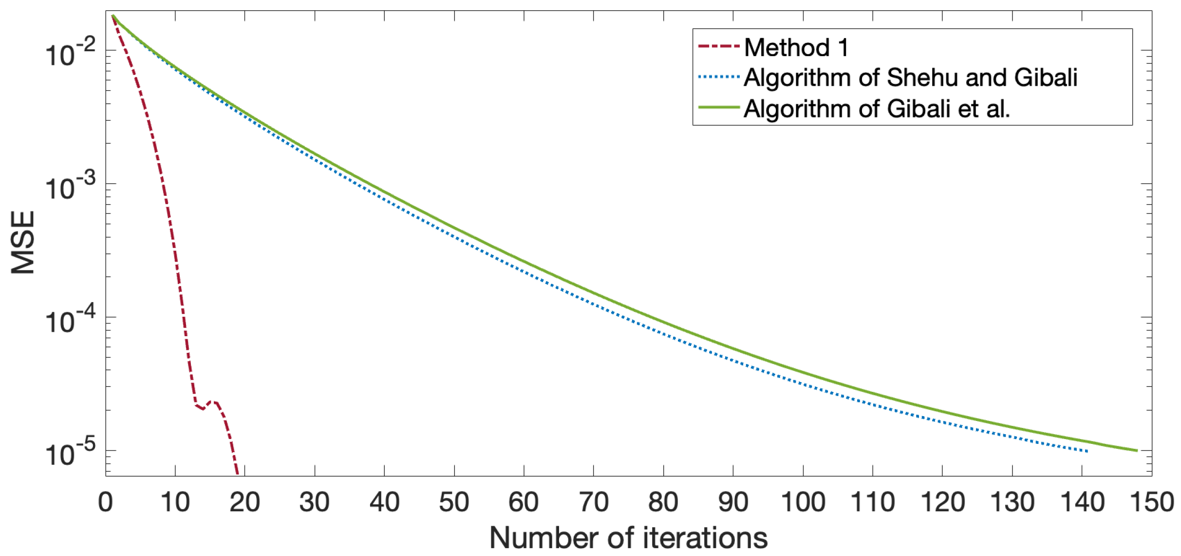
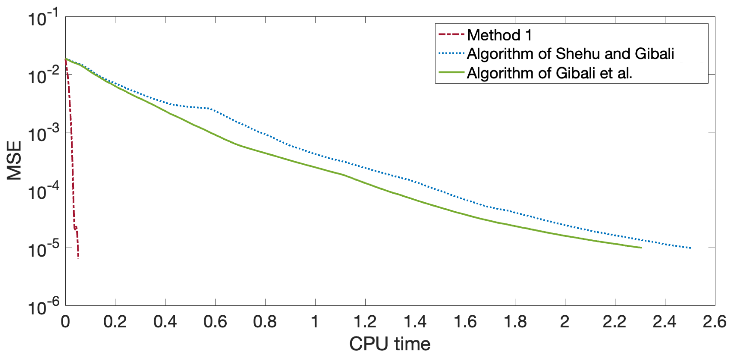
4. Numerical Experiments

Next, we give a comparison with algorithm of Gibali et al. [22], and the algorithm of Shehu and Gibali [25] for signal recovery, which is modeled as follows:

$${\displaystyle \underset{s\in {\mathbb{R}}^P}{min}\frac{1}{2}{\parallel t-As\parallel }^2\mathrm{subject}\mathrm{to}{\parallel s\parallel }_1\le e,}$$

(40)

where $s\in {\mathbb{R}}^P$ is a recovered vector with m nonzero components, $t\in {\mathbb{R}}^K$ are the observed data, $e>0$ is a given constant, and A is an $K\times P$ matrix with $K<P$.

We see that if let $C=\{s\in {\mathbb{R}}^P:{\parallel s\parallel }_1\le e\}$ and $Q=\left\{t\right\}$; then, (40) can be reduced to SFP.

Sparse vector $s\in {\mathbb{R}}^P$ is constructed by the uniform distribution in $[-2,2]$ with m nonzero elements. Matrix A is constructed by normal distribution with mean zero and variance one. Let t be the white Gaussian noise with SNR = 40. Let $e=m$ and initial point $s_0=s_1=(0,0,0,...,0)\in {\mathbb{R}}^P$. We use the mean square error (MSE):

$${\displaystyle MSE=\frac{1}{P}{\parallel s_k-s^{*}\parallel }^2,}$$

(41)

where $s_k$ is an estimated signal of $s^{*}$.

In the algorithm of Gibali et al. [22], and the algorithm of Shehu and Gibali [25], we choose $\gamma =1$, $\ell =\mu =0.5$. In Method 1, ${\beta }_k$ defined by a fast iterative shrinkage-thresholding algorithm (FISTA) [31]. Choose ${\rho }_1=0.1$, $\mu =0.4$, $\sigma =0.8$ and set

$${\beta }_k=\left\{\begin{array}{cc}\frac{a_{k-1}-1}{a_k},\hfill & \mathrm{if}1\le k\le 1000\hfill \\ 0\hfill & \mathrm{otherwise}.\hfill \end{array}\right.$$

where $a_0=1$, $a_k=\frac{1+\sqrt{1+4a_{k-1}^2}}{2}$. Numerical experiments were carried out in MATLAB version R2020b on MacBook Pro M1 with ram 8 GB. The numerical results are given by the following tables.

Table 1. Comparison of iteration (Iter) for $P=2048$, $K=1024$ and different m-sparse, $MSE<{10}^{-3}$ and $MSE<{10}^{-5}$.

m-Sparse	Methods	$\mathit{MSE}<{10}^{-3}$	$\mathit{MSE}<{10}^{-5}$
		Iter	Iter
m = 10	Method 1	6	11
	Algorithm of Shehu and Gibali [25]	15	73
	Algorithm of Gibali et al. [22]	16	77
m = 20	Method 1	8	17
	Algorithm of Shehu and Gibali [25]	29	89
	Algorithm of Gibali et al. [22]	30	94
m = 30	Method 1	9	19
	Algorithm of Shehu and Gibali [25]	41	141
	Algorithm of Gibali et al. [22]	43	148

and

Table 2. Results of MSE values, objective function values, and CPU time in seconds for each method and each iteration ($P=2048$, $K=1024$, $m=30$, $MSE<{10}^{-5}$).

Methods	Iter	MSE Values		Objective Functions
		MSE	CPU	Obj	CPU
Method 1	1	0.0185	0.0002	1.8832 × 10${}^4$	0.0007
	2	0.0130	0.0052	3.8504 × 10${}^3$	0.0050
	3	0.0097	0.0094	1.8248 × 10${}^3$	0.0091
	4	0.0070	0.0126	1.0359 × 10${}^3$	0.0125
	⋮	⋮	⋮	⋮	⋮
	19	6.4529 × 10${}^{-6}$	0.0524	0.0746	0.0522
Algorithm of Shehu and Gibali [25]	1	0.0185	0.0006	1.8832 × 10${}^4$	0.0007
	2	0.0159	0.0372	1.2047 × 10${}^4$	0.0364
	3	0.0144	0.0676	7.4679 × 10${}^3$	0.0665
	4	0.0128	0.0864	5.5536 × 10${}^3$	0.0862
	⋮	⋮	⋮	⋮	⋮
	141	9.8423 × 10${}^{-6}$	2.5043	0.6112	2.5041
Algorithm of Gibali et al. [22]	1	0.0185	0.0002	1.8832 × 10${}^4$	0.0011
	2	0.0159	0.0312	1.2047 × 10${}^4$	0.0303
	3	0.0144	0.0593	7.4679 × 10${}^3$	0.0582
	4	0.0130	0.0766	5.7134 × 10${}^3$	0.0765
	⋮	⋮	⋮	⋮	⋮
	148	9.9682 × 10${}^{-6}$	2.3068	0.6227	2.3067

show that Method 1 had less iteration, CPU time, and lower objective function and MSE values than those of the algorithm of Shehu and Gibali [25], and the algorithm of Gibali et al. [22] for different m-sparse. This reveals that our algorithm had better convergence than that of other methods.

We next provide the convergence behavior, MSE, number of iterations, objective function values, and CPU time.

In Figure 1, Figure 2, Figure 3 and Figure 4, we see that Method 1 converged to a solution faster than the algorithms in [22,25] did.

We next show the illustration of the original signal and recovered signal by Method 1, the algorithm of Shehu and Gibali [25], and the algorithm of Gibali et al. [22] when $MSE<{10}^{-3}$.

From Figure 5, the results include the recovery signal via Method 1, and the algorithm in [22,25].

5. Conclusions

In this work, we improved using the projection method by a new inertial step and a new hybrid step size. We gave a weak convergence theorem under suitable conditions for solving split feasibility. We applied the result to signal recovery and provided a comparison with other methods. Results showed that our method is more efficient than other methods in terms of iteration and CPU time.

References

1. Byrne, C.; Moudafi, A. Extensions of the CQ algorithm for the split feasibility and split equality problems. Doc. Trav. 2013, 18, 1485–1496. [Google Scholar]
2. Censor, Y.; Gibali, A.; Lenzen, F.; Schnörr, C. The implicit convex feasibility problem and its application to adaptive image denoising. J. Comput. Math. 2016, 34, 610–625. [Google Scholar] [CrossRef] [Green Version]
3. O’Hara, J.G.; Pillay, P.; Xu, H.K. Iterative approaches to convex feasibility problems in Banach spaces. Nonlinear Anal. Theory Methods Appl. 2006, 64, 2022–2042. [Google Scholar] [CrossRef]
4. Tian, D.; Jiang, L. Two-step methods and relaxed two-step methods for solving the split equality problem. Comput. Appl. Math. 2021, 40, 83. [Google Scholar] [CrossRef]
5. Censor, Y.; Elfving, T. A multiprojection algorithm using Bregman projections in a product space. Numer. Algorithms 1994, 8, 221–239. [Google Scholar] [CrossRef]
6. Ansari, Q.H.; Rehan, A. An iterative method for split hierarchical monotone variational inclusions. Fixed Point Theory Appl. 2015, 2015, 121. [Google Scholar] [CrossRef] [Green Version]
7. Censor, Y.; Elfving, T.; Kopf, N.; Bortfeld, T. The multiple-sets split feasibility problem and its applications for inverse problems. Inverse Probl. 2005, 21, 2071. [Google Scholar] [CrossRef] [Green Version]
8. Censor, Y.; Bortfeld, T.; Martin, B.; Trofimov, A. A unified approach for inversion problems in intensity-modulated radiation therapy. Phys. Med. Biol. 2006, 51, 2353. [Google Scholar] [CrossRef] [PubMed] [Green Version]
9. Censor, Y.; Motova, A.; Segal, A. Perturbed projections and subgradient projections for the multiple-sets split feasibility problem. J. Math. Anal. Appl. 2007, 327, 1244–1256. [Google Scholar] [CrossRef] [Green Version]
10. Gu, R.; Dogandžić, A. Projected nesterov’s proximal-gradient algorithm for sparse signal recovery. IEEE Trans. Signal Process. 2017, 65, 3510–3525. [Google Scholar] [CrossRef]
11. Ceng, L.C.; Ansari, Q.H.; Yao, J.C. An extragradient method for solving split feasibility and fixed point problems. Comput. Math. Appl. 2012, 64, 633–642. [Google Scholar] [CrossRef] [Green Version]
12. Dang, Y.; Gao, Y. The strong convergence of a KM–CQ-like algorithm for a split feasibility problem. Inverse Probl. 2010, 27, 015007. [Google Scholar] [CrossRef]
13. Gibali, A.; Mai, D.T. A new relaxed CQ algorithm for solving split feasibility problems in Hilbert spaces and its applications. J. Ind. Manag. Optim. 2019, 15, 963. [Google Scholar] [CrossRef] [Green Version]
14. Kesornprom, S.; Pholasa, N.; Cholamjiak, P. On the convergence analysis of the gradient-CQ algorithms for the split feasibility problem. Numer. Algorithms 2020, 84, 997–1017. [Google Scholar] [CrossRef]
15. Kesornprom, S.; Cholamjiak, P. On inertial relaxation CQ algorithm for split feasibility problems. Commun. Math. Appl. 2019, 10, 245–255. [Google Scholar]
16. Qu, B.; Xiu, N. A new halfspace-relaxation projection method for the split feasibility problem. Linear Algebra Its Appl. 2008, 428, 1218–1229. [Google Scholar] [CrossRef] [Green Version]
17. Suparatulatorn, R.; Cholamjiak, W.; Gibali, A.; Mouktonglang, T. A parallel Tseng’s splitting method for solving common variational inclusion applied to signal recovery problems. Adv. Differ. Equ. 2021, 2021, 492. [Google Scholar] [CrossRef]
18. Yambangwai, D.; Khan, S.A.; Dutta, H.; Cholamjiak, W. Image restoration by advanced parallel inertial forward-backward splitting methods. Soft Comput. 2021, 25, 6029–6042. [Google Scholar] [CrossRef]
19. Byrne, C. Iterative oblique projection onto convex sets and the split feasibility problem. Inverse Probl. 2002, 18, 441. [Google Scholar] [CrossRef]
20. Yang, Q. The relaxed CQ algorithm solving the split feasibility problem. Inverse Probl. 2004, 20, 1261. [Google Scholar] [CrossRef]
21. Zhao, J.; Zhang, Y.; Yang, Q. Modified projection methods for the split feasibility problem and the multiple-sets split feasibility problem. Appl. Math. Comput. 2012, 219, 1644–1653. [Google Scholar] [CrossRef]
22. Gibali, A.; Liu, L.W.; Tang, Y.C. Note on the modified relaxation CQ algorithm for the split feasibility problem. Optim. Lett. 2018, 12, 817–830. [Google Scholar] [CrossRef]
23. López, G.; Martín-Márquez, V.; Wang, F.; Xu, H.K. Solving the split feasibility problem without prior knowledge of matrix norms. Inverse Probl. 2012, 28, 085004. [Google Scholar] [CrossRef]
24. Nesterov, Y.E. A method for solving the convex programming problem with convergence rate O(1/k2). Dokl. Akad. Nauk SSSR 1983, 269, 543–547. [Google Scholar]
25. Shehu, Y.; Gibali, A. New inertial relaxed method for solving split feasibilities. Optim. Lett. 2021, 15, 2109–2126. [Google Scholar] [CrossRef]
26. Bauschke, H.H.; Combettes, P.L. Convex Analysis and Monotone Operator Theory in Hilbert Spaces; Springer: New York, NY, USA, 2011; Volume 408. [Google Scholar]
27. Osilike, M.O.; Aniagbosor, S.C.; Akuchu, B.G. Fixed points of asymptotically demicontractive mappings in arbitrary Banach spaces. Panam. Math. J. 2002, 12, 77–88. [Google Scholar]
28. Hanjing, A.; Suantai, S. A fast image restoration algorithm based on a fixed point and optimization method. Mathematics 2020, 8, 378. [Google Scholar] [CrossRef] [Green Version]
29. Bauschke, H.H.; Combettes, P.L. A weak-to-strong convergence principle for Fejér-monotone methods in Hilbert spaces. Math. Oper. Res. 2001, 26, 248–264. [Google Scholar] [CrossRef] [Green Version]
30. Alvarez, F.; Attouch, H. An inertial proximal method for maximal monotone operators via discretization of a nonlinear oscillator with damping. Set-Valued Anal. 2001, 9, 3–11. [Google Scholar] [CrossRef]
31. Beck, A.; Teboulle, M. A fast iterative shrinkage-thresholding algorithm for linear inverse problems. SIAM J. Imaging Sci. 2009, 2, 183–202. [Google Scholar] [CrossRef] [Green Version]
Figure 1. Graph of MSE and number of iterations for P = 2048 , K = 1024 , m = 30 when M S E < 10 5 .
Mathematics 10 00933 g001
Figure 2. Graph of objective function values and number of iterations for P = 2048 , K = 1024 , m = 30 when M S E < 10 5 .
Mathematics 10 00933 g002
Figure 3. Graph of MSE values and CPU time for P = 2048 , K = 1024 , m = 30 when M S E < 10 5 .
Mathematics 10 00933 g003
Figure 4. Graph of the objective function values and CPU time for P = 2048 , K = 1024 , m = 30 when M S E < 10 5 .
Mathematics 10 00933 g004
Figure 5. Original signal and recovered signal by Method 1, algorithm of Shehu and Gibali and algorithm of Gibali et al., respectively, when P = 2048 , K = 1024 , m = 30 and M S E < 10 3 . (a) Recovered signal by Method 1. (b) Recovered signal by the algorithm of Shehu and Gibali. (c) Recovered signal by the algorithm of Gibali et al.
Mathematics 10 00933 g005