On a New Family of Runge–Kutta–Nyström Pairs of Orders 6(4)

Abstract

In this study, Runge–Kutta–Nyström pairs of orders 6(4) using six stages per step are considered. The main contribution of the present work is that we introduce a new family of pairs (i.e., new methodology of solution for order conditions) that possesses seven free parameters instead of four, as used by similar pairs until now. Using these extra coefficients efficiently we may construct methods with better properties. Here, we exploit the free parameters in order to derive a pair with extended imaginary stability interval. This type of method may furnish better results on problems with periodic solutions. Extended numerical tests justify our effort.

1. Introduction

The second order initial value problem with the special form

$$y^{″}=f(x,y),y\left(x_0\right)=y_0,y^{\prime }\left(x_0\right)=y_0^{\prime }$$

(1)

where $f:ℝ\times {ℝ}^m\to {ℝ}^m$, and $(y_0,y_0^{\prime })\in {ℝ}^{2m}$, is under consideration here.

We make an approximation to the solution of problem (1) at a collection of separate points $\left(x_n,y_n,y_n^{\prime }\right)$ using an explicit Runge–Kutta–Nyström (RKN) pair sharing algebraic orders $p\left(q\right)$, $p>q$. The format of this method is as follows [1]

$$f_i=f(x_n+c_i{h}_n,y_n+c_i{h}_n{y}_n^{\prime }+h_n^2\sum _{j=1}^s{\tilde{\alpha }}_{ij}{f}_j),i=1,2,\cdots ,s$$

$$\begin{array}{cc}{y}_{n+1}=y_n+h_n{y}_n^{\prime }+h_n^2\sum _{i=1}^s{w}_i{f}_i,\hfill & {\widehat{y}}_{n+1}=y_n+h_n{y}_n^{\prime }+h_n^2\sum _{i=1}^s{\widehat{w}}_i{f}_i,\hfill \\ y_{n+1}^{\prime }=y_n^{\prime }+h_n\sum _{i=1}^s{w}_i^{\prime }{f}_i,\hfill & {\widehat{y}}_{n+1}^{\prime }=y_n^{\prime }+h_n\sum _{i=1}^s{\widehat{w}}_i^{\prime }{f}_i,\hfill \end{array}$$

where $h_n=x_{n+1}-x_n,$ is the stepsize. The higher order approximations $y_n,y_n^{\prime }$ are used to propagate the solutions. The weights $\widehat{w}$ and ${\widehat{w}}^{\prime }$ furnish the lower accuracy approximations used for error estimation.

The latter can be computed by the expression

$${ϵ}_n=h_n^{p-q+1}·max(\parallel h_n^2\sum _{i=1}^s(w_i-{\widehat{w}}_i)f_i\parallel ,\parallel h_n\sum _{i=1}^s(w_i^{\prime }-{\widehat{w}}_i^{\prime })f_i)\parallel ,$$

and the compared can be a very small positive number $TOL$ set by the user of the pair. Then, using this small number, called tolerance, we may guess the length of the next step length

$$h_{n+1}=0.9·h_n·{\left(\frac{TOL}{{ϵ}_n}\right)}^{1/p}.$$

In the exceptional case when $TOL<{ϵ}_n$, we do not allow the solution to propagate. We actually repeat the current step and use $h_{n+1}$ instead of $h_n$ as its new and shorter version.

All the coefficients can be formulated using the Butcher tableau [2,3]. So, the method takes the form

with $\tilde{A}\in {ℝ}^{s\times s}$, $w^{\mathrm{T}}, {\widehat{w}}^{\mathrm{T}}, w^{\prime \mathrm{T}}, {\widehat{w}}^{\mathrm{T}}, c\in {ℝ}^s.$

Pairs of orders six and four (i.e., $p=6$ and $q=4$) were studied in [1,4]. There, pairs DEP6(4) and PT6(4) were respectively presented. The following Butcher tableau characterizes these pairs.

From the tableau above it can be seen that the last stage (i.e., the sixth) shares as coefficients the vector w. These are actually six stages pairs (i.e., $s=6$) using the FSAL (First Stage As Last) device. Thus, only five stages are wasted every step. The PT6(4) pair was specially designed to address periodic problems since it shares higher phase-lag order. Reducing the phase lag we try to keep the difference in angles between the theoretical and numerical solution small when integrating harmonic oscillator.

In the following we are interested to study a six stages (i.e., $s=6$) pair of orders six and four (i.e., $p=6$ and $q=4$). These pairs are shown in the following Butcher tableaus

Such pairs were firstly studied in [5]. No FSAL device is used on these pairs. In [5] all the coefficients are expressed with respect to four free parameters that can be chosen arbitrarily. Namely $c_3,c_4,c_5$ and $w_6^{\prime }$. The pair ER6(4) was presented there, achieving small local truncation errors. However, it seems that we may use seven free parameters for constructing pairs of this form, as will be seen below. We aim to exploit these extra parameters for achieving long imaginary stability intervals.

2. The New Family of Runge–Kutta–Nyström Pairs Sharing Orders 6(4)

According to the relevant theory, there are 47 equations of condition for achieving a pair of orders six and four [5,6]. We may consider the simplifying assumption

$$\tilde{A}·e=\frac{1}{2}{c}^2,$$

(2)

with $e={[1,1,\cdots ,1]}^T\in {ℝ}^s$ and $c^2=c\ast c$ the component wise multiplication between the elements of vector c. Then the number of order conditions reduces to just 29. Another common assumption is

$$w=w^{\prime }·(I_s-\mathrm{diag}\left(c\right)),\widehat{w}={\widehat{w}}^{\prime }·(I_s-\mathrm{diag}\left(c\right)),$$

(3)

with $I_s\in {ℝ}^{s\times s}$ the identity matrix. After (3) holds, only 18 equations remain to be solved. Namely, 13 of them correspond to the higher order formula:

The 1st, 2nd, and 3rd order conditions, respectively.

$$w^{\prime }·e=1,w^{\prime }·c=\frac{1}{2},w^{\prime }·c^2=\frac{1}{3}.$$

The 4th order conditions.

$$w^{\prime }·c^3=\frac{1}{4},w^{\prime }·\tilde{A}·c=\frac{1}{24}.$$

The 5th order conditions.

$$w^{\prime }·c^4=\frac{1}{5},w^{\prime }·(c\ast \tilde{A}·c)=\frac{1}{30},w^{\prime }·\tilde{A}·c^2=\frac{1}{60}.$$

The 6th order conditions.

$$w^{\prime }·c^5=\frac{1}{6},w^{\prime }·\left(c^2\ast \tilde{A}·c\right)=\frac{1}{36},w^{\prime }·\left(c\ast \tilde{A}·c^2\right)=\frac{1}{72},$$

$$w^{\prime }·\tilde{A}·c^3=\frac{1}{120},w^{\prime }·{\tilde{A}}^2·c=\frac{1}{720}.$$

Whereas for the lower order formula, the following five equations must be satisfied,

$${\widehat{w}}^{\prime }·e=1,{\widehat{w}}^{\prime }·c=\frac{1}{2},{\widehat{w}}^{\prime }·c^2=\frac{1}{3},{\widehat{w}}^{\prime }·c^3=\frac{1}{4},{\widehat{w}}^{\prime }·\tilde{A}·c=\frac{1}{24}.$$

In these equations, “∗” is to be understood as a component-wise multiplication among vectors and has the lowest priority after all other operations. Also, $c^2=c\ast c$, $c^3=c^2\ast c$, etc. This latter operation (“raising” a vector to a power) has the highest priority and is evaluated before dot products and “∗”.

The parameters available are 25. Specifically

$$c_2,c_3,c_4,c_5,{\tilde{\alpha }}_{32},{\tilde{\alpha }}_{42},{\tilde{\alpha }}_{43},{\tilde{\alpha }}_{52},{\tilde{\alpha }}_{53},{\tilde{\alpha }}_{54},{\tilde{\alpha }}_{62},{\tilde{\alpha }}_{63},{\tilde{\alpha }}_{64},{\tilde{\alpha }}_{65},w_1^{\prime },w_2^{\prime },w_3^{\prime },w_4^{\prime },w_5^{\prime },w_6^{\prime },{\widehat{w}}_1^{\prime },{\widehat{w}}_2^{\prime },{\widehat{w}}_3^{\prime },{\widehat{w}}_4^{\prime },{\widehat{w}}_6^{\prime }.$$

Thus, we may choose 7 of them arbitrarily. We select $c_2,c_3,c_4,c_5,{\tilde{\alpha }}_{62},{\tilde{\alpha }}_{63}$ and ${\tilde{\alpha }}_{64}$ as free parameters. Then we may explicitly evaluate all the remaining coefficients. The algorithm for this is as follows.

Firstly, set

$${\tilde{\alpha }}_{65}=-\frac{\left\{\begin{array}{c}(c_2-1)(c_3-1)(c_4-1){(c_5-1)}^2(c_2(5c_3(2c_4-1)-5c_4+3)\\ +c_3(3-5c_4)+3c_4-2)\end{array}\right\}}{\left\{\begin{array}{c}2c_5(c_5-c_2)(c_3-c_5)(c_5-c_4)\left(c_2\right(5c_3(6c_4{c}_5-4c_4-4c_5+3)\\ -20c_4{c}_5+15c_4+15c_5-12)+c_3(-20c_4{c}_5+15c_4+15c_5-12)\\ +15c_4{c}_5-12c_4-12c_5+10)\end{array}\right\}}.$$

Continue evaluating $w_1^{\prime },w_2^{\prime },w_3^{\prime },w_4^{\prime },w_5^{\prime }$, and $w_6^{\prime }$ after solving the linear system

$$w^{\prime }·e=1,w^{\prime }·c=\frac{1}{2},w^{\prime }·c^2=\frac{1}{3},w^{\prime }·c^3=\frac{1}{4},w^{\prime }·c^4=\frac{1}{5},w^{\prime }·c^5=\frac{1}{6}.$$

The remaining six equations (except $w^{\prime }·{\tilde{A}}^2·c=\frac{1}{720}$) for the higher order formula can also be solved explicitly, since they are linear in ${\tilde{a}}_{32},{\tilde{a}}_{42},{\tilde{a}}_{43},{\tilde{a}}_{52},{\tilde{a}}_{53},{\tilde{a}}_{54}$. The 13th equation was already satisfied by ${\tilde{a}}_{65}$. The remaining coefficients of the first column of $\tilde{A}$ (i.e., ${\tilde{a}}_{21}$, ${\tilde{a}}_{31}$, ${\tilde{a}}_{41}$, ${\tilde{a}}_{51}$ and ${\tilde{a}}_{61}$) are found by expression (2).

We proceed by evaluating the weights of the lower order formula. Thus, we set

$${\widehat{w}}_5^{\prime }=\frac{\left\{\begin{array}{c}{c}_4(c_2-c_4)(2{\tilde{a}}_{32}{c}_2(6c_2{c}_4-4c_2-4c_4+3)+c_3(c_2-c_3)(c_3-c_4))\\ -2{\tilde{a}}_{42}{c}_2{c}_3\left(c_2^2(6c_3-4)+c_2\left(3-6c_3^2\right)+c_3(4c_3-3)\right)\\ +2{\tilde{a}}_{43}{c}_3^2\left(c_2^2(4-6c_3)+c_2\left(6c_3^2-3\right)+(3-4c_3)c_3\right)\end{array}\right\}}{24\left(\begin{array}{c}{\tilde{a}}_{32}{c}_2^3{c}_4^2{c}_5-{\tilde{a}}_{32}{c}_2^3{c}_4{c}_5^2-{\tilde{a}}_{32}{c}_2^2{c}_4^3{c}_5+{\tilde{a}}_{32}{c}_2^2{c}_4{c}_5^3+{\tilde{a}}_{32}{c}_2{c}_4^3{c}_5^2-{\tilde{a}}_{32}{c}_2{c}_4^2{c}_5^3\\ -{\tilde{a}}_{42}{c}_2^3{c}_3^2{c}_5+{\tilde{a}}_{42}{c}_2^3{c}_3{c}_5^2+{\tilde{a}}_{42}{c}_2^2{c}_3^3{c}_5-{\tilde{a}}_{42}{c}_2^2{c}_3{c}_5^3-{\tilde{a}}_{42}{c}_2{c}_3^3{c}_5^2+{\tilde{a}}_{42}{c}_2{c}_3^2{c}_5^3\\ -{\tilde{a}}_{43}{c}_2^2{c}_3^3{c}_5+{\tilde{a}}_{43}{c}_2^2{c}_3^2{c}_5^2+{\tilde{a}}_{43}{c}_2{c}_3^4{c}_5-{\tilde{a}}_{43}{c}_2{c}_3^2{c}_5^3-{\tilde{a}}_{43}{c}_3^4{c}_5^2+{\tilde{a}}_{43}{c}_3^3{c}_5^3\\ +{\tilde{a}}_{52}{c}_2{c}_3{c}_4(c_2-c_3)(c_2-c_4)(c_3-c_4)\\ +{\tilde{a}}_{53}{c}_3^2{c}_4(c_2-c_3)(c_2-c_4)(c_3-c_4)+{\tilde{a}}_{54}{c}_2^2{c}_3^2{c}_4^2-{\tilde{a}}_{54}{c}_2^2{c}_3{c}_4^3\\ -{\tilde{a}}_{54}{c}_2{c}_3^3{c}_4^2+{\tilde{a}}_{54}{c}_2{c}_3{c}_4^4+{\tilde{a}}_{54}{c}_3^3{c}_4^3-{\tilde{a}}_{54}{c}_3^2{c}_4^4\end{array}\right)}$$

and conclude by finding ${\widehat{w}}_1^{\prime },{\widehat{w}}_2^{\prime },{\widehat{w}}_3^{\prime },{\widehat{w}}_4^{\prime },$ after solving the linear system

$${\widehat{w}}^{\prime }·e=1,{\widehat{w}}^{\prime }·c=\frac{1}{2},{\widehat{w}}^{\prime }·c^2=\frac{1}{3},{\widehat{w}}^{\prime }·c^3=\frac{1}{4},$$

with respect to these parameters.

Finally, the coefficients in vectors w and $\widehat{w}$ can be found explicitly by expressions (3).

3. Stability Intervals

Having at hand seven free coefficients instead of four we may exploit them in various directions. Here, we will try to derive a pair that performs best on periodic problems.

Following Horn [7] or Dormand et al. [1], we consider the test problem $y^{″}={\mu }^{2}y$ (with $\mu$ complex). Since $y^{\prime }=\mu y$, we conclude to the following recursions for y and $y^{\prime }$,

$$\begin{array}{ccc}\hfill y_{n+1}& =& \left\{1+v^{2}w{\left(I-v^2\tilde{A}\right)}^{-1}e+v\left(1+v^{2}w{\left(I-v^2\tilde{A}\right)}^{-1}c\right)\right\} · y_n=R\left(v\right) · y_n,\hfill \\ \hfill y_{n+1}^{\prime }& =& \left\{v{w}^{\prime }{\left(I-v^2\tilde{A}\right)}^{-1}e+\left(1+v^2{w}^{\prime }{\left(I-v^2\tilde{A}\right)}^{-1}c\right)\right\} · y_n^{\prime }=R^{\ast }\left(v\right) · y_n^{\prime },\hfill \end{array}$$

with $v=\mu h$. Thus, the RKN methods posses a couple of stability regions associated with their higher orders formulas. Namely, for y and $y^{\prime }$. We may produce them requiring $\left|R\right(v\left)\right|<1$ and $|R^{\ast }\left(v\right)|<1$. This type of stability analysis is associated to the corresponding A-stability of Runge–Kutta methods.

Let, for $i\ge 1$,

$${\delta }_{2i-1}=w{\tilde{A}}^{i-1}e,{\delta }_{2i}=w{\tilde{A}}^{i-1}c,{\delta }_{2i-1}^{\prime }=w^{\prime }{\tilde{A}}^{i-1}e,{\delta }_{2i}^{\prime }=w^{\prime }{\tilde{A}}^{i-1}c,$$

with ${\delta }_{-1}^{\prime }=0,{\delta }_0={\delta }_{-1}={\delta }_0^{\prime }=1$. Applying the formal Neumann expansion of ${\left(I-zA\right)}^{-1}$ and since $\tilde{A}$ is strictly lower triangular, we may write

$$R\left(v\right)=1+v+\frac{1}{2}{v}^2+\frac{1}{6}{v}^3+\frac{1}{24}{v}^4+\frac{1}{120}{v}^5+\frac{1}{720}{v}^6+{\delta }_6{v}^7+{\delta }_7{v}^8+{\delta }_8{v}^9+{\delta }_9{v}^{10},$$

$$R^{\ast }\left(v\right)=1+v+\frac{1}{2}{v}^2+\frac{1}{6}{v}^3+\frac{1}{24}{v}^4+\frac{1}{120}{v}^5+\frac{1}{720}{v}^6+{\delta }_7^{\prime }{v}^7+{\delta }_8^{\prime }{v}^8+{\delta }_9^{\prime }{v}^9+{\delta }_{10}^{\prime }{v}^{10}+{\delta }_{11}^{\prime }{v}^{11}.$$

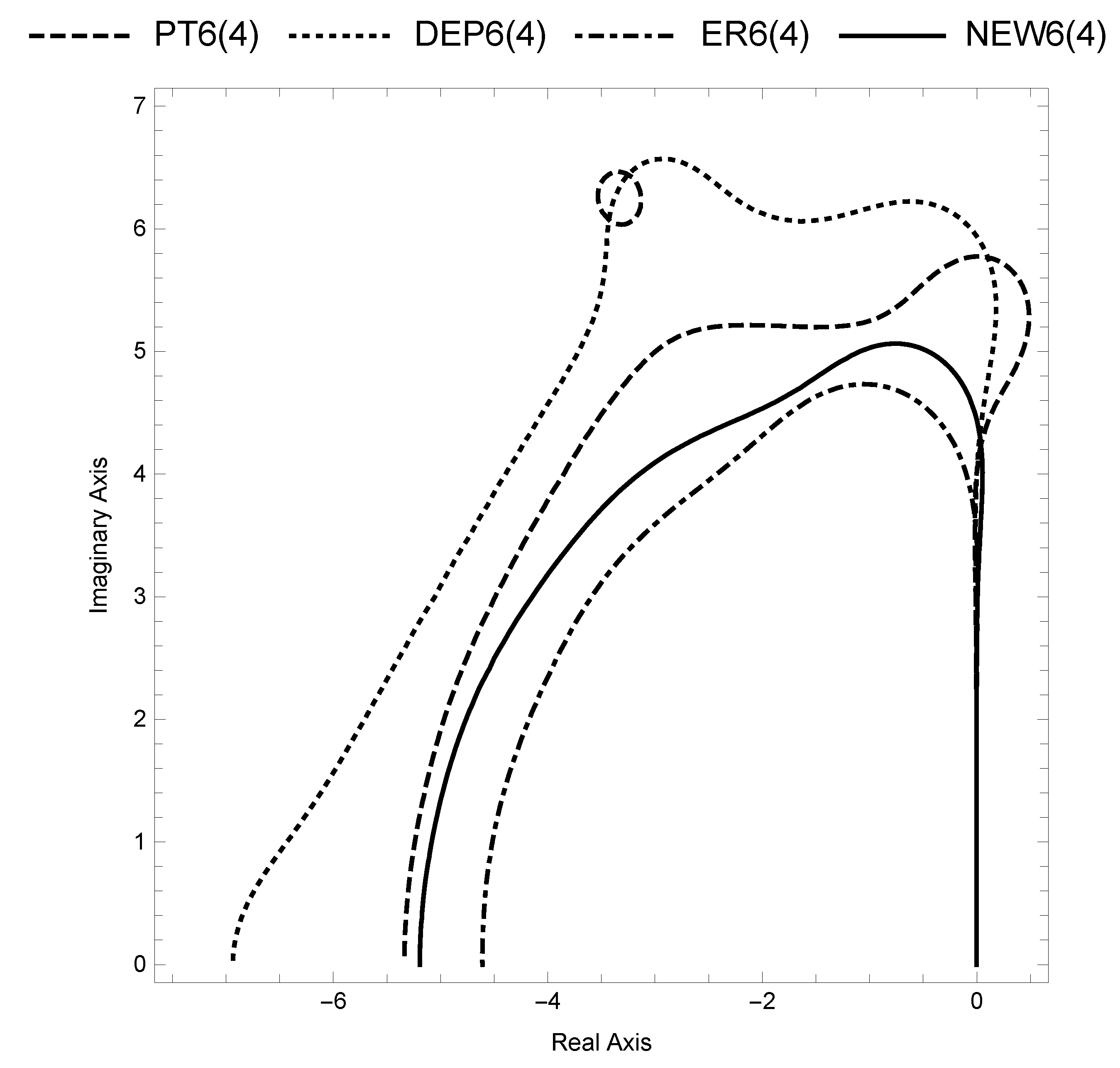
The stability region defined by $R\left(v\right)$ is characterized by its first cuts (i.e., those closest to origin) with the two axes, i.e., the real and imaginary axes. Thus, we define the corresponding intervals. Namely (i) the real stability interval $(-\tilde{v},0)$ (ii) the imaginary stability interval $(0,\widehat{v})$ with both $\tilde{v}$ and $\widehat{v}$ being real numbers. Analogously we define the corresponding intervals $(-{\tilde{v}}^{\ast },0)$ and $(0,{\widehat{v}}^{\ast })$ associated with $R^{\ast }\left(v\right)$.

We focus on pairs with long imaginary stability intervals since such pairs are expected to perform better on periodic problems. For deriving such a method we expressed $R\left(v\right)$ and $R^{\ast }\left(v\right)$ with respect to the free parameters and v. Let us assume $v=v\sqrt{-1}$, $v\in ℝ$, i.e., concentrate on the imaginary axis. Then, for a sixth order method, we conclude to

$${\left|R\left(v\right)\right|}^2={(1-\frac{v^2}{2}+\frac{v^4}{24}-\frac{v^6}{720}+{\delta }_7{v}^8-{\delta }_9{v}^{10})}^2+{(v-\frac{v^3}{6}+\frac{v^5}{120}-{\delta }_6{v}^7+{\delta }_8{v}^9)}^2$$

and

$$|R^{\ast }{\left(v\right)|}^2={(1-\frac{v^2}{2}+\frac{v^4}{24}-\frac{v^6}{720}+{\delta }_8^{\prime }{v}^8-{\delta }_{10}^{\prime }{v}^{10})}^2+{(v-\frac{v^3}{6}+\frac{v^5}{120}-{\delta }_7^{\prime }{v}^7+{\delta }_9^{\prime }{v}^9-{\delta }_{11}^{\prime }{v}^{11})}^2.$$

Then, we used Differential Evolution Algorithm [8,9] for maximizing v with respect to ${\left|R\left(v\right)\right|}^2\le 1$ and $|R^{\ast }{\left(v\right)|}^2\le 1$. We manage to get such a pair (named NEW6(4)) with coefficients presented in the Appendix A as part of a MATLAB [10] listing.

In fact, we compute with these coefficients

$$\begin{array}{ccc}\hfill {\left|R\left(v\right)\right|}^2& \approx & \\ & & {\left(\begin{array}{c}1-v^2/2+v^4/24-v^6/720\\ +2.477993886208964524\times {10}^{-5}{v}^8-2.15355114080193519\times {10}^{-7}{v}^{10}\end{array}\right)}^2\hfill \\ & & +{\left(\begin{array}{c}v-v^3/6+v^5/120\\ +1.984043154492196\times {10}^{-4}{v}^7-2.5011619564014669781\times {10}^{-6}{v}^9\end{array}\right)}^2.\hfill \end{array}$$

Observe that ${\left|R\left(v\right)\right|}^2\le 1$ for $v\in [0,5.39]$ and thus we get an imaginary stability interval for y. Analogously, we may work for $y^{\prime }$.

The main characteristics of the major RKN pairs of orders 6(4) that have appeared until now in the literature are given in

Table 1. Basic characteristics of the RKN Pairs considered.

Pair	Stages	${∥{\mathit{T}}^{(\mathit{p}+1)}∥}_2$	${∥{\mathit{T}}^{\prime }{}^{(\mathit{p}+1)}∥}_2$	$\widehat{\mathit{v}}$	${\widehat{\mathit{v}}}^{\ast }$	$\tilde{\mathit{v}}$	${\tilde{\mathit{v}}}^{\ast }$
PT6(4) [4]	5	$8.4\times {10}^{-5}$	$6.7\times {10}^{-5}$	4.39	0	5.32	5.33
DEP6(4) [1]	5	$8.7\times {10}^{-5}$	$7.7\times {10}^{-5}$	3.27	0	6.95	6.93
ER6(4) [5]	6	$4.9\times {10}^{-9}$	$4.8\times {10}^{-9}$	1.82	0	4.61	4.61
NEW6(4)	6	$1.1\times {10}^{-5}$	$1.4\times {10}^{-5}$	5.39	4.44	5.13	5.19

$\hat{v}$: Length of Imaginary Stability Interval associated with y. ${\hat{v}}^{\ast }$: Length of Imaginary Stability Interval associated with y′. $\tilde{v}$: Length of Real Stability Interval associated with y. ${\tilde{v}}^{\ast }$: Length of Real Stability Interval associated with y′. ${∥T^{(p+1)}∥}_2$: Euclidean norm of the vector consisting of all the principal truncation error coefficients of the higher order method of a pair (regarding the solution y). ${∥T^{\prime }{}^{(p+1)}∥}_2$: as before, but regarding y′.

. As can be seen there, they do not posses an imaginary stability interval for $y^{\prime }$. In addition, the new pair has longer stability interval for y. The corresponding regions are presented in Figure 1 and Figure 2.

4. Numerical Tests

We tested the following pairs

• The five stages (effectively) pair PT6(4) given in [4];
• The five stages (effectively) pair DEP6(4) given in [1];
• The six stages pair ER6(4) given in [5];
• The six stages Runge–Kutta–Nyström pairs of orders 6(4) presented here.

The problems with periodic solutions selected for tests are the following. All these examples were tested using the listing in the Appendix A and changing only the coefficients in the preamble according to the pair under consideration.

(A)

The model problem

$$y^{″}=-9y,y\left(0\right)=1,y^{\prime }\left(0\right)=0,x\in [0,10\pi ],$$

with analytical solution $y\left(x\right)=cos\left(3x\right)$. We integrated the problem in the interval $x\in \left[0,10\pi \right]$ for tolerances ${10}^{-5},{10}^{-6},\cdots ,{10}^{-11}$.

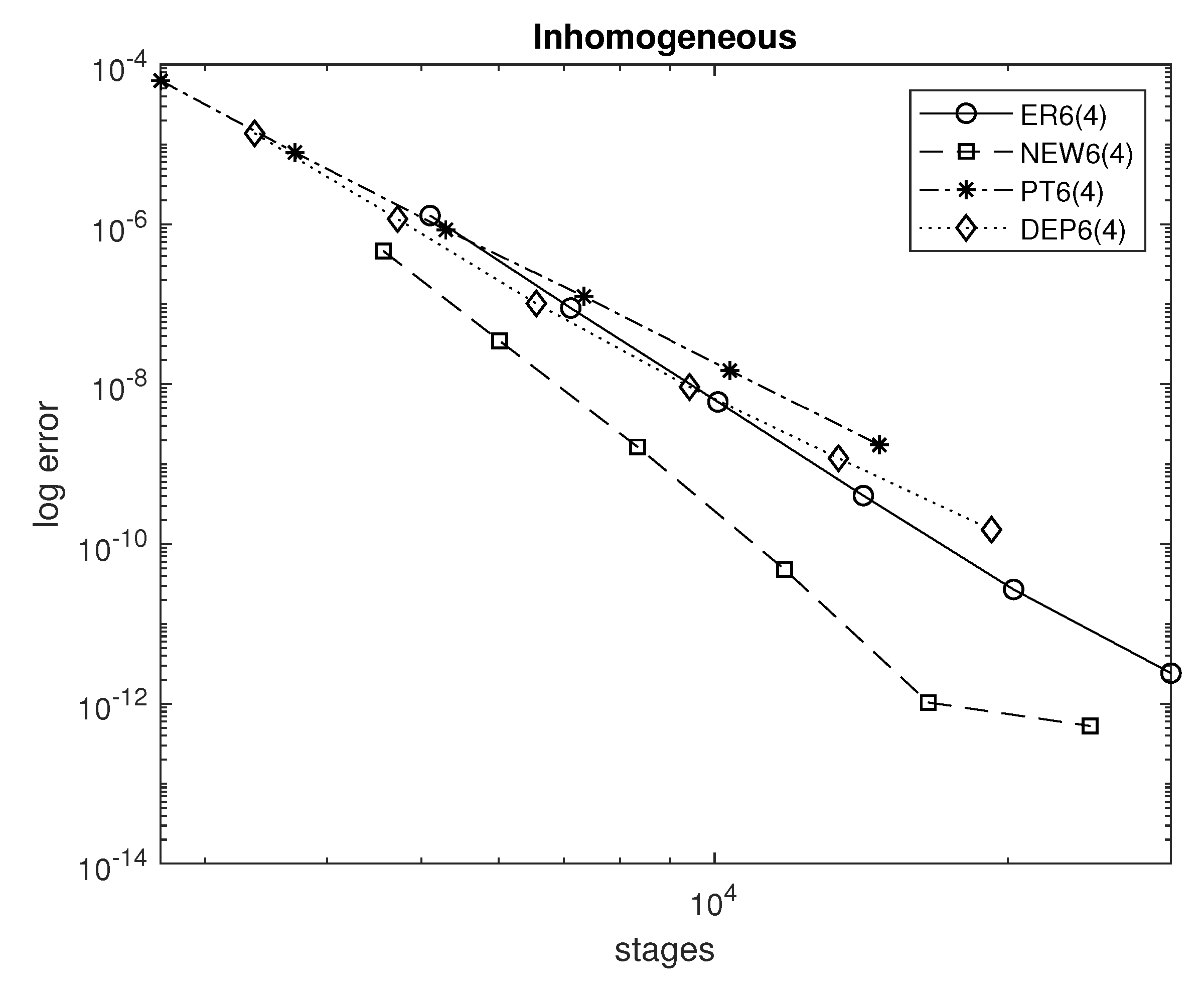
The efficiency plot recording the stages used by the four pairs versus the maximum global errors observed over the whole grid is presented in Figure 3. All figures of efficiency plots are in log-log scale.

(B)

In-homogeneous problem [11]

$$y^{″}\left(x\right)=-100y\left(x\right)+99sin\left(x\right),y\left(0\right)=1,y^{\prime }\left(0\right)=11,$$

with analytical solution

$$y\left(x\right)=cos\left(10x\right)+sin\left(10x\right)+sin\left(x\right).$$

We integrated the problem in the interval $x\in \left[0,10\pi \right]$ for tolerances ${10}^{-5},{10}^{-6},\cdots ,$ ${10}^{-11}$. The efficiency plot recording the stages used by the four pairs versus the maximum global errors observed over the whole grid is presented in Figure 4.

(C)

Bessel problem [12]

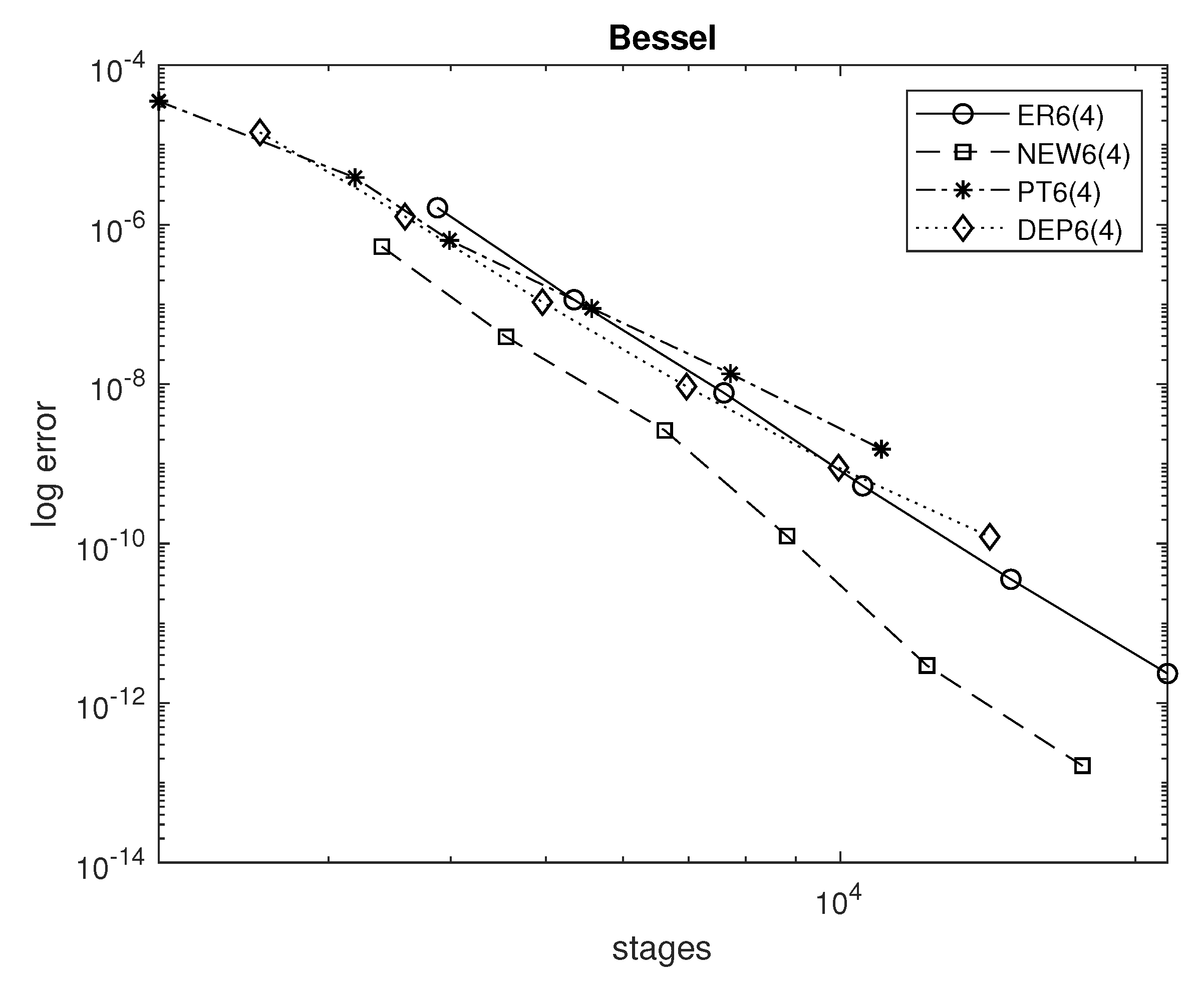
The well known Bessel equation

$$y^{″}=-y\left(x\right)·\frac{1+400x^2}{4x^2},$$

is verified by an analytical solution of the form

$$y\left(x\right)=J_0\left(10x\right)·\sqrt{x},$$

with $J_0$ being the zeroth order Bessel function of the first kind. We solved the above equation in the interval $\left[1,10\pi \right]$ for tolerances ${10}^{-5},{10}^{-6},\cdots ,{10}^{-11}$. The efficiency plot recording the stages used by the four pairs versus the maximum global errors observed over the whole grid is presented in Figure 5.

(D)

The Duffing equation

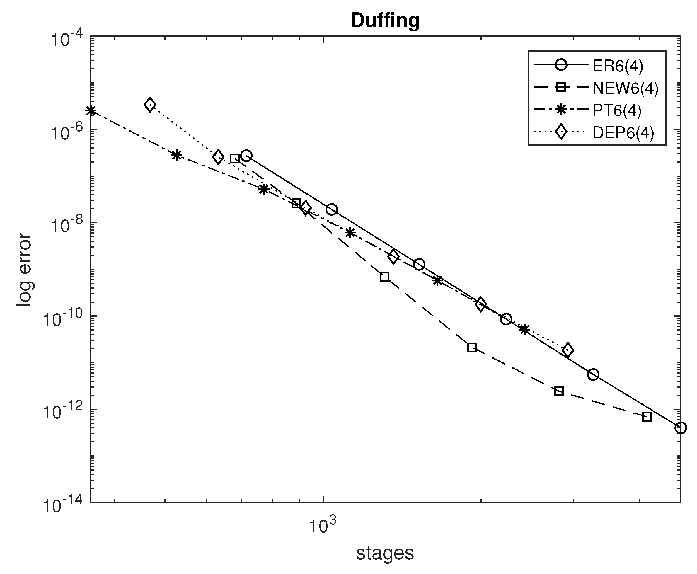
Next, we choose the equation [13]

$$\begin{array}{c}\hfill y^{″}\left(x\right)=-y\left(x\right)-y{\left(x\right)}^3+\frac{1}{500}·cos\left(1.01x\right),\\ \hfill y\left(0\right)=0.2004267280699011,y^{\prime }\left(0\right)=0,\end{array}$$

with an approximate analytical solution

$$y\left(x\right)\approx \begin{array}{c}0.2001794775368452cos\left(1.01x\right)+2.469461432611\times {10}^{-4}cos\left(3.03x\right)\\ +3.040149839\times {10}^{-7}cos\left(5.05x\right)+3.743495\times {10}^{-10}cos\left(7.07x\right)\\ +4.609\times {10}^{-13}cos\left(9.09x\right)+6\times {10}^{-16}cos\left(11.11x\right).\end{array}$$

We solved the above equation in the interval $\left[0,\frac{20.5}{1.01}\pi \right]$ for tolerances ${10}^{-5},{10}^{-6},\cdots ,$ ${10}^{-11}$. The efficiency plot recording the stages used by the four pairs versus the maximum global errors observed over the whole grid is presented in Figure 6.

(E)

semi-Linear system

The nonlinear problem proposed by Franco and Gomez [14] follows.

$$\begin{array}{ccc}\hfill y^{″}\left(x\right)& =& \left(\begin{array}{cc}-199& -198\\ 99& 98\end{array}\right)·y\left(x\right)+\left(\genfrac{}{}{0pt}{}{{\left(y_1+y_2\right)}^2+{sin}^2\left(10x\right)-1}{{\left(y_1+2y_2\right)}^2-{10}^{-6}sin{}^2\left(x\right)}\right),\hfill \\ \hfill x& \in & \left[0,10\pi \right],\hfill \end{array}$$

with theoretical solution

$$y\left(x\right)=\left(\begin{array}{c}2cos\left(10x\right)-{10}^{-3}sin\left(x\right)\\ -cos\left(10x\right)+{10}^{-3}sin\left(x\right)\end{array}\right).$$

Notice that $y_1,y_2$ may be understood here as components of vector y. We solved the above equation in the interval $\left[0,\frac{20.5}{1.01}\pi \right]$ for tolerances ${10}^{-5},{10}^{-6},\cdots ,{10}^{-10}$. The efficiency plot recording the stages used by the four pairs versus the maximum global errors observed over the whole grid is presented in Figure 7.

(F)

Wave equation

We finally consider the Wave equation of the form [15],

$$\begin{array}{ccc}\hfill \frac{{\partial }^{2}y}{\partial t^2}& =& 4\frac{{\partial }^{2}y}{\partial r^2}+sint·cos\left(\frac{\pi r}{100}\right),0\le r\le 100,t\in [0,10\pi ],\hfill \\ \hfill \frac{\partial y}{\partial r}\left(t,0\right)& =& \frac{\partial y}{\partial r}\left(t,100\right)=0\hfill \\ \hfill y\left(0,r\right)& \equiv & 0,\frac{\partial y}{\partial t}\left(0,r\right)=\frac{{100}^2}{4{\pi }^2-{100}^2}cos\frac{\pi r}{100},\hfill \end{array}$$

with the exact solution

$$y\left(t,r\right)=\frac{{100}^2}{4{\pi }^2-{100}^2}·sin\left(t\right)·cos\frac{\pi r}{100}.$$

We semi-discretisize $\frac{{\partial }^{2}y}{\partial r^2}$ with fourth order symmetric differences at internal points and one sided differences of the same order at the boundaries and conclude to the system:

$$\begin{array}{ccc}\hfill \left[\begin{array}{c}{y}_1^{″}\hfill \\ y_2^{″}\hfill \\ \\ \\ y_{N+1}^{″}\hfill \end{array}\right]& =& \frac{4}{{\left(\mathsf{\Delta }r\right)}^2}\left[\begin{array}{cccccccc}-\frac{415}{72}& 8& -3& \frac{8}{9}& -\frac{1}{8}& 0& \cdots & \\ \frac{257}{144}& -\frac{10}{3}& \frac{7}{4}& -\frac{2}{9}& \frac{1}{48}& 0& \cdots & \\ -\frac{1}{12}& \frac{4}{3}& -\frac{5}{2}& \frac{4}{3}& -\frac{1}{12}& & & ⋮\\ 0& & \ddots & \ddots & \ddots & \ddots & \ddots & 0\\ ⋮& & & -\frac{1}{12}& \frac{4}{3}& -\frac{5}{2}& \frac{4}{3}& -\frac{1}{12}\\ & \cdots & 0& \frac{1}{48}& -\frac{2}{9}& \frac{7}{4}& -\frac{10}{3}& \frac{257}{144}\\ & \cdots & 0& -\frac{1}{8}& \frac{8}{9}& -3& 8& -\frac{415}{72}\end{array}\right]·\left[\begin{array}{c}{y}_1\\ y_2\\ ⋮\\ \\ y_{N+1}\end{array}\right]\hfill \\ & & +sint·\left[\begin{array}{c}cos\left(\frac{0·\mathsf{\Delta }r}{r}·\pi \right)\\ cos\left(\frac{1·\mathsf{\Delta }r}{r}·\pi \right)\\ ⋮\\ \\ cos\left(\frac{N·\mathsf{\Delta }r}{r}·\pi \right)\end{array}\right].\hfill \end{array}$$

By choosing $\mathsf{\Delta }r=\frac{1}{4}$ we arrive at a constant coefficients linear system with $N=401.$ Then $y_1\approx y(t,0)$, $y_2\approx y(t,\mathsf{\Delta }r)$, $y_3\approx y(t,2\mathsf{\Delta }r),\cdots$, $y_{401}\approx y(t,400\mathsf{\Delta }r)$. In addition, here $y_1,y_2,\cdots$ may be understood as components of vector y.

We solved the above equation in the interval $\left[0,10\pi \right]$ for tolerances ${10}^{-7.5},{10}^{-8},\cdots ,$ ${10}^{-9.5},{10}^{-10}$. The efficiency plot recording the stages used by the four pairs versus the maximum global errors observed over the whole grid is presented in Figure 8.

The wave equation is a mildly stiff problem. This explains the peculiar performance of the pairs. The maximum accuracy is limited due to the space discretezation error there. Even so, the new pair reaches it faster. Lower order finite difference methods (e.g., Crank–Nicolson) have difficulties in attaining such high accuracies as NEW6(4).

The overall results indicate the superiority of the new pair over non stiff problems with periodic solutions.

It is standard in RKN literature to present comparisons with stages vs. error. This is independent from the hardware used and programming issues. Besides, some runs here ended after very few stages and the timing might be unreliable even using the same machine. In the following we present a couple of figures (in log-log scale) with efficiency plots including times vs. accuracies. The tests were carried on AMD Ryzen 9-3900X, 12-Core Processor at 3.79 GHz. Parallel computation of MATLAB was not applied in time or space direction of the problems.

The similarity of the above Figure 9 and Figure 10 with the corresponding Figure 5 and Figure 7, respectively, is indicative.

5. Conclusions

We considered the Runge–Kutta–Nyström pairs of orders 6(4) for addressing the special second order Initial Value Problem. We focused on problems with periodic solutions. Thus, we proposed a new family of such pairs and derived a certain representative with extended imaginary stability regions. The extensive results justified our effort.

References

- Dormand, J.R.; El-Mikkawy, M.E.A.; Prince, P.J. Families of Runge-Kutta-Nyström formulae. IMA J. Numer. Anal. 1987, 7, 235–250. [Google Scholar] [CrossRef]
- Butcher, J.C. On Runge-Kutta processes of high order. J. Aust. Math. Soc. 1964, 4, 179–194. [Google Scholar] [CrossRef] [Green Version]
- Butcher, J.C. Numerical Methods for Ordinary Differential Equations, 3rd ed.; John Wiley & Sons: Chichester, UK, 2016. [Google Scholar]
- Papakostas, S.N.; Tsitouras, C. High phase-lag order Runge-Kutta and Nyström pairs. SIAM J. Sci. Comput. 1999, 21, 747–763. [Google Scholar] [CrossRef]
- El-Mikkawy, M.E.A.; Rahmo, E. A new optimized non-FSAL embedded Runge-Kutta-Nyström algorithm of orders 6 and 4 in six stages. Appl. Math. Comput. 2003, 145, 3343. [Google Scholar] [CrossRef]
- Fehlberg, E. Eine Runge-Kutta-Nystrom-Formel g-ter Ordnung rnit Schrittweitenkontrolle fur Differentialgleichungen = f(t,x). ZAMM 1981, 61, 477–485. [Google Scholar] [CrossRef]
- Horn, M.K. Developments in High Order Runge-Kutta-Nystrom Formulas. Ph.D. Thesis, The University of Texas, Austin, TX, USA, 1977. [Google Scholar]
- Storn, R.; Price, K. Differential evolution—A simple and efficient heuristic for global optimization over continuous spaces. J. Glob. Optim. 1997, 11, 341–359. [Google Scholar] [CrossRef]
- Storn, R.; Price, K.; Neumaier, A.; Zandt, J.V. DeMat. Available online: https://www.swmath.org/software/24853 (accessed on 23 August 2021).
- Matlab. MATLAB Version 7.10.0; The MathWorks Inc.: Natick, MA, USA, 2010. [Google Scholar]
- Van de Vyver, H. Scheifele two-step methods for perturbed oscillators. J. Comput. Appl. Math. 2009, 224, 415–432. [Google Scholar] [CrossRef] [Green Version]
- Van de Vyver, H. A Runge-Kutta-Nyström pair for the numerical integration of perturbed oscillators. Comput. Phys. Commun. 2005, 167, 129–142. [Google Scholar] [CrossRef]
- Vanden Berghe, G.; Van Daele, M. Exponentially-fitted Obrechkoff methods for second-order differential equations. Appl. Numer. Math. 2009, 59, 815–829. [Google Scholar] [CrossRef]
- Franco, J.M.; Gomez, I. Trigonometrically fitted nonlinear two-step methods for solving second order oscillatory IVPs. Appl. Math. Comput. 2014, 232, 643–657. [Google Scholar] [CrossRef]
- Simos, T.E.; Tsitouras, C. Explicit, Ninth Order, Two Step Methods for solving Inhomogeneous Linear problems x″(t) = Λx(t) + f(t). Appl. Numer. Math. 2020, 153, 344–351. [Google Scholar] [CrossRef]