Finite-Time Synchronization Analysis for BAM Neural Networks with Time-Varying Delays by Applying the Maximum-Value Approach with New Inequalities

Abstract

In this paper, we consider the finite-time synchronization for drive-response BAM neural networks with time-varying delays. Instead of using the finite-time stability theorem and integral inequality method, by using the maximum-value method, two new criteria are obtained to ensure the finite-time synchronization for the considered drive-response systems. The inequalities in our paper, applied to obtaining the maximum-valued and designing the novel controllers, are different from those in existing papers.

1. Introduction

In 1987, Kosko firstly proposed a two-way associative search for stored bipolar vector pairs and generalized the single-layer auto-associative Hebbian correlation to a two-layer pattern-matched hetero-associative circuit. These are a class of important neural networks, called bidirectional associative memory (BAM) neural networks [1,2]. The dynamic behaviors of BAM neural networks are of significant application prospects in various fields, such as automatic control, signal processing, pattern recognition and associative memory, which has arisen the great interest of researchers. To date, many researchers have analyzed various dynamical behaviors of BAM neural networks, and obtained many dynamical analysis results of BAM neural networks [3,4,5,6,7,8,9,10,11,12,13,14,15,16,17,18,19,20,21,22,23,24,25,26,27,28,29,30,31,32,33,34,35,36,37,38,39,40,41,42,43,44,45,46,47,48,49,50]. In recent years, the global asymptotic/exponential synchronization of BAM neural networks has been widely investigated, for example, see [3,4,5,6,7,8,9,10,11,12,13] and references therein. Meanwhile, many scholars have devoted themselves to the study of the finite-time synchronization of BAM neural networks, for example, see [14,15,16,17,18,19,20,21,22,42] and references therein.

In [14], the authors developed a finite-time synchronization for the drive–response fuzzy inertial BAM neural networks by employing integral inequality techniques and the figure analysis approach. Furthermore, the finite-time stochastic synchronization for memristor-based BAM neural networks with time-varying delays and stochastic disturbances was considered in [15]. In addition, the authors built more reasonable switching conditions of the finite-time synchronization by using a stochastic analysis technique. In [16], researchers introduced a different inequality, the fractional-order Gronwall inequality with time delays, and then dealt with the finite-time synchronization problem of fractional-order memristor-based neural networks with time delays. Zhang and Yang [17] studied the finite-time impulsive synchronization issue of fractional-order memristive BAM neural networks involving switch jumps mismatch by designing two impulsive controllers and using the properties of Gamma functions. In [18], the finite-time synchronization of drive–response BAM fuzzy neural networks with time delays and impulsive effects was investigated. The authors’ goal was to illustrate the effects of both impulse and time delay in a finite-time control area in terms of novel Lyapunov functionals and special analytical techniques. Motivated by security applications in the image transmission, Wang et al. [19] provided some sufficient conditions to guarantee the finite-time projective synchronization for memristor-based BAM neural networks.

So far, the investigated results about the finite-time synchronization of BAM neural networks and non-BAM neural networks have been acquired mainly by applying Lyapunov functionals [15,18], analysis approaches [15,17,18], inequality approaches [14,16,19,21,22], the finite-time stability theorem [20,21] and the integral inequality method [48,49,50]. Recently, two novel sufficient conditions were obtained to guarantee the finite-time synchronization for the considered drive–response fuzzy inertial neural networks by using the maximum-value approach [42].

Inspired by [42], we studied the finite-time synchronization of BAM neural networks by applying the maximum-value approach. In this paper, by using different inequality techniques from those in [42] and designing controllers different from those in [14,15,16,17,18,19,20,21,22,42], the finite-time synchronization criteria for drive–response BAM neural networks with time-varying delays are obtained. In proving the main results, one of the two difficulties in our paper was how to construct novel inequalities in the controllers to get $V^{\prime }(t)<\psi (t)$ and the other one was how to establish the new inequalities in the controllers to achieve a finite-time synchronization. Thus, the novelty of this paper is to construct some novel inequalities to obtain the maximum value of the considered functions and to get the finite time $t_1$ needed to achieve synchronization. As a result, the main contribution of this paper lies in the following three aspects:

(1) Some new inequalities which are different from those in [42] are constructed in the process of obtaining the maximum-value of the considered functions; (2) new inequalities described with fractional and integral functions are introduced to design the novel controllers; (3) using the maximum-value approach and designing novel controllers, two different conditions are attained to assure the finite-time synchronization between the drive system and the response system.

The rest of this paper is arranged as follows. In Section 2, some necessary preliminaries are given. In Section 3, two novel criteria to realize the finite-time synchronization are put forward for the drive system (1) and the response system (2). In Section 4, we exhibit two examples to validate the effectiveness and feasibility of the derived consequences.

2. Preliminaries

In this paper, we consider a class of BAM neural networks with time-varying delays described by

$$\left\{\begin{array}{c}\frac{d{x}_i(t)}{dt}=-a_i{x}_i(t)+{\displaystyle \sum _{j=1}^m}{c}_{ij}{f}_j(y_j(t))+{\displaystyle \sum _{j=1}^m}{d}_{ij}{f}_j(y_j(t-{\tau }_{ji}(t)))+I_i,\\ \frac{d{y}_j(t)}{dt}=-b_j{y}_j(t)+{\displaystyle \sum _{i=1}^n}{p}_{ji}{g}_i(x_i(t))+{\displaystyle \sum _{i=1}^n}{q}_{ji}{g}_i(x_i(t-{\sigma }_{ij}(t)))+J_j,\end{array}\right.$$

(1)

where $i=1,2,\cdots ,n,j=1,2,\cdots ,m,a_i>0$ and $b_j>0$ are constants; $x_i(t),y_j(t)$ are the states of the ith neuron and jth neuron; constants $c_{ij},d_{ij},p_{ji},q_{ji}$ denote the connection strengths; ${\tau }_{ji}(t),{\sigma }_{ij}(t)$ are time delays, $0<{\sigma }_{ij}^{\prime }(t)<{\sigma }^{*},0<{\tau }_{ji}^{\prime }(t)<{\tau }^{*}$; functions $f_j,g_i$ denote the activation functions; constants $I_i,J_j$ denote the external inputs.

The initial values of system (1) are given as follows:

$$x_i(s)={\varphi }_{xi}(s),s\in [-\sigma ,0],y_j(s)={\psi }_{yj}(s),s\in [-\tau ,0],$$

where $\sigma =\underset{1\le i\le n,1\le j\le m}{max}\{{\sigma }_{ij}(t)\},\tau =\underset{1\le i\le n,1\le j\le m}{max}\{{\tau }_{ji}(t)\},{\varphi }_{xi}(s),{\psi }_{yj}(s)$ are bounded continuous functions.

Throughout this paper, for system (1), we always assume that

Zhen: have modified. $(H_1)$ There exist constants $F_j>0,G_i>0$ such that

$$|f_j(x)-f_j(y)|\le F_j|x-y|,|g_i(x)-g_i(y)|\le G_i|x-y|,$$

for all $x,y\in R,i=1,2,\cdots ,n,j=1,2,\cdots ,m,|.|$ is the norm of the Euclidean space $R.$

For simplicity, we refer to (1) as the drive system, and consider the response BAM neural networks with time-varying delays described as follows:

$$\left\{\begin{array}{c}\frac{d{u}_i(t)}{dt}=-a_i{u}_i(t)+{\displaystyle \sum _{j=1}^m}{c}_{ij}{f}_j(v_j(t))+{\displaystyle \sum _{j=1}^m}{d}_{ij}{f}_j(v_j(t-{\tau }_{ji}(t)))+I_i+P_i(t),\\ \frac{d{v}_j(t)}{dt}=-b_j{v}_j(t)+{\displaystyle \sum _{i=1}^n}{p}_{ji}{g}_i(u_i(t))+{\displaystyle \sum _{i=1}^n}{q}_{ji}{g}_i(u_i(t-{\sigma }_{ij}(t)))+J_j+Q_j(t),\end{array}\right.$$

(2)

where $u_i(t),v_j(t)$ denote the states, the parameters are the same as those in system (1) and $P_i(t),Q_j(t)$ are the controllers to realize finite-time synchronization between the drive system (1) and the response system (2).

The initial values of system (2) are given as follows:

$$u_i(s)={\varphi }_{ui}(s),s\in [-\sigma ,0],v_j(s)={\psi }_{vj}(s),s\in [-\tau ,0],$$

where $\sigma =\underset{1\le i\le n,1\le j\le m}{max}\{{\sigma }_{ij}(t)\},\tau =\underset{1\le i\le n,1\le j\le m}{max}\{{\tau }_{ji}(t)\},{\varphi }_{ui}(s),{\psi }_{vj}(s)$ are bounded continuous functions.

Definition 1.

Drive–response systems (1) and (2) are said to be finite-time synchronized if for arbitrary solutions of system (1) and system (2) denoted by $[x_1(t),x_2(t),\cdots ,x_n(t),y_1(t),y_2(t),$$\cdots ,y_m{(t)]}^T$ and ${[u_1(t),u_2(t),\cdots ,u_n(t),v_1(t),v_2(t),\cdots ,v_m(t)]}^T$, under a suitable designed controller, there exists a time $T>0$ which is related to the initial condition, such that for $i=1,2,\cdots ,n;j=1,2,\cdots ,m$,

$$\underset{t\to T}{lim}|u_i(t)-x_i(t)|=0;\underset{t\to T}{lim}|v_j(t)-y_j(t)|=0;$$

$$|u_i(t)-x_i(t)|=0,t>T;|v_j(t)-y_j(t)|=0,t>T.$$

Lemma 1

([51]). If $x>0,y>0,p>1,\frac{1}{p}+\frac{1}{k}=1,k$ is a constant, then

$$xy\le \frac{x^p}{p}+\frac{y^k}{k}.$$

Lemma 2.

If $a>1,b>1,$ and $\frac{1}{a}+\frac{1}{b}=1,$ when $t>\frac{3}{4}$, the following inequality holds:

$$ln(4t+1)+1-2ln2<\frac{1}{a}{(t+\frac{1}{4})}^a+\frac{1}{b}.$$

Proof. 

Let $f(t)=\frac{1}{a}{(t+\frac{1}{4})}^a+\frac{1}{b}-ln(4t+1)-1+2ln2,t>\frac{3}{4}.$ Then $f^{\prime }(t)={(t+\frac{1}{4})}^{a-1}-\frac{4}{4t+1},t>\frac{3}{4}.$ Thus, $f^{″}(t)=\frac{16}{{(4t+1)}^2}\left[(a-1){(t+\frac{1}{4})}^{a+1}\right]>0,t>\frac{3}{4}.$ So $f^{\prime }(t)$ is a monotonically increasing function on $(\frac{3}{4},+\infty )$ and then $f^{\prime }(t)>f^{\prime }(\frac{3}{4})=0$. Therefore, when $t>\frac{3}{4}$, $f(t)$ is also a monotonically increasing function and $f(t)>f(\frac{3}{4})=0.$ Finally, $ln(4t+1)+1-2ln2<\frac{1}{a}{(t+\frac{1}{4})}^a+\frac{1}{b}$ holds. □

Lemma 3.

If $t\ge \frac{1}{e},a^{*}>\frac{1+e}{e^{\frac{1}{e}}-1},$ then $t+1+a^{*}t-a^{*}t{e}^t<0.$

Proof. 

We only need to prove $max\left\{\frac{1+t}{t(e^t-1)}\right\}\le \frac{1+e}{e^{\frac{1}{e}}-1}$.

Denote $F(t)=\frac{1+t}{t(e^t-1)}$. Then, we have $F^{\prime }(t)=\frac{1-e^t-t^2{e}^t-t{e}^t}{t^2{(e^t-1)}^2}<0,t\ge \frac{1}{e}$.

Hence, $F(t)$ is a monotonically decreasing function on $[\frac{1}{e},+\infty )$.

Furthermore, $F(t)\le F(\frac{1}{e})=\frac{1+e}{e^{\frac{1}{e}}-1}<a^{*}$. □

Lemma 4

([42]). Assume that z = f(x) defined on $(-\infty ,+\infty )$, and $x_0$ is a unique local maximum value point. Then, $\underset{x\in (-\infty ,+\infty )}{max}f(x)=max\{f(x_0);f(-\infty );f(+\infty )\}$.

Proof. 

The proof is well-known and it is omitted. □

3. Main Results

Let $e_i(t)=u_i(t)-x_i(t),r_j(t)=v_j(t)-y_j(t)$, then the error system can be described as follows:

$$\left\{\begin{array}{c}\frac{d{e}_i(t)}{dt}=-a_i{e}_i(t)+{\displaystyle \sum _{j=1}^m}{c}_{ij}\left[f_j(v_j(t))-f_j(y_j(t))\right]+{\displaystyle \sum _{j=1}^m}{d}_{ij}[f_j(v_j(t-{\tau }_{ji}(t)))\\ -f_j(y_j(t-{\tau }_{ji}(t)))]+P_i(t),\\ \frac{d{r}_j(t)}{dt}=-b_j{r}_j(t)+{\displaystyle \sum _{i=1}^n}{p}_{ji}\left[g_i(u_i(t))-g_i(x_i(t))\right]+{\displaystyle \sum _{i=1}^n}{q}_{ji}[g_i(u_i(t-{\sigma }_{ij}(t)))\\ -g_i(x_i(t-{\sigma }_{ij}(t)))]+Q_j(t).\end{array}\right.$$

(3)

The controllers in system (3) are designed as follows for $i=1,2,\cdots ,n,j=1,2,\cdots ,m$:

$$\left\{\begin{array}{c}{P}_i\left(t\right)=sign\left[e_i\left(t\right)\right]k_1+k_2{e}_i\left(t\right)+sign\left[e_i\left(t\right)\right]{\left|e_i\left(t\right)\right|}^{1-p}{k}_3,e_i\left(t\right)\ne 0,\\ Q_j\left(t\right)=sign\left[r_j\left(t\right)\right]l_1+l_2{r}_j\left(t\right)+sign\left[r_j\left(t\right)\right]\times {\left|r_j\left(t\right)\right|}^{1-p}\frac{\varphi \left(t\right)}{p}+\\ sign\left[r_j\left(t\right)\right]{\left|r_j\left(t\right)\right|}^{1-p}{l}_3,r_j\left(t\right)\ne 0\end{array}\right.$$

(4)

or

$$\left\{\begin{array}{c}{P}_i\left(t\right)={\left[e_i\left(t\right)\right]}^{-1}{w}_1+w_2{e}_i\left(t\right)+{\left[e_i\left(t\right)\right]}^{1-2q}{w}_3,e_i\left(t\right)\ne 0,\\ Q_j\left(t\right)={\left[r_j\left(t\right)\right]}^{-1}{z}_1+z_2{r}_j\left(t\right)+{\left[r_j\left(t\right)\right]}^{1-2q}\frac{\psi \left(t\right)}{2q}+\\ {\left[r_j\left(t\right)\right]}^{1-2q}{z}_3,r_j\left(t\right)\ne 0\end{array}\right.$$

(5)

where $p\ge 1,\varphi \left(t\right)=\frac{4}{4t+1}-{(t+\frac{1}{4})}^{a-1}-1,t\ge \frac{3}{4},a>1,b>1,$ and $\frac{1}{a}+\frac{1}{b}=1,$ $p{k}_3+k_1^p{\left(\frac{p-1}{-A_i}\right)}^{p-1}<0,$ $p{l}_3+l_1^p{\left(\frac{p-1}{-B_j}\right)}^{p-1}<0,$ $k_1>0,$ $k_2<0,$ $k_3<0,$ $l_1>0,$ $l_2<0,$ $l_3<0;$ $q\ge 1,$ $\psi \left(t\right)=1+a^{*}-a^{*}(e^t+t{e}^t)-e^t-3M\left(0\right),$ $t\ge \frac{1}{e},$ $a^{*}\ge \frac{1+e}{e^{\frac{1}{e}}-1},$ $2q{w}_3+w_1^q{2}^q{\left(\frac{q-1}{-C_i}\right)}^{2q-1}<0,$ $2q{z}_3+z_1^q{2}^q{\left(\frac{q-1}{-D_i}\right)}^{q-1}<0,$ $w_1>0,$ $w_2<0,$ $w_3<0,$ $z_1>0,$ $z_2<0,$ $z_3<0,$ $A_i,B_j$ are defined in Theorem 1, $C_i,D_j,M\left(t\right)$ are defined in Theorem 2 and $M\left(0\right)$ is the value when $t=0$ in $M\left(t\right)$.

Notation 1.

In (4), $\varphi \left(t\right)$ is independent of the initial values of the error systems, while in (5), $\psi \left(t\right)$ is dependent on the initial values of the error systems, so the controllers (4) and the controllers (5) are different. Under these two controllers, the finite-time synchronization for the drive system (1) and the response system (2) are achieved under some conditions.

Theorem 1.

Assume the condition $\left(H_1\right)$ holds. Then, the drive system (1) and the response system (2) are finite-time synchronized under the controllers (4) in a finite time $t_1$, where $t_1=max\left\{\frac{3}{4},\frac{V\left(0\right)}{m}+2ln2-1+\frac{1}{b}+\frac{1}{a}·\frac{1}{4^a}\right\}$ if there exists a positive constant $p\ge 1$ such that the following conditions hold:

$\left(H_2\right)$

$$A_i=(k_2-a_i)p+(p-1)\sum _{j=1}^m{F}_j(|c_{ij}|+|d_{ij}|)+G_i\sum _{j=1}^m(|p_{ji}|+\frac{1}{1-{\sigma }^{*}}|q_{ji}|)<0;$$

$(H_3)$

$$B_j=(l_2-b_j)p+(p-1)\sum _{i=1}^n{G}_i(|p_{ji}|+|q_{ji}|)+F_j\sum _{i=1}^n(|c_{ij}|+\frac{1}{1-{\tau }^{*}}|d_{ij}|)<0.$$

Proof. 

Without loss of generalization, we assume that $e_i(t)\ne 0,r_j(t)\ne 0$ (If $e_i(t)=0,r_j(t)=0,$ then the finite-time synchronization has been proved (if $e_i(t)=0$ or $r_j(t)=0,$ then the proof is a special case of the following proof).

We construct a Lyapunov function as follows:

$$V(t)=V_1(t)+V_2(t),$$

where,

$$V_1(t)=\sum _{i=1}^n|e_i{(t)|}^p+\sum _{j=1}^m{|r_j(t)|}^p,$$

$$V_2(t)=\frac{1}{1-{\tau }^{*}}\sum _{i=1}^n\sum _{j=1}^m|d_{ij}|F_j{\int }_{t-{\tau }_{ji}(t)}^t|r_j{(s)|}^{p}ds+\frac{1}{1-{\sigma }^{*}}\sum _{i=1}^n\sum _{j=1}^m|q_{ji}|G_i{\int }_{t-{\sigma }_{ij}(t)}^t{|e_i(s)|}^{p}ds.$$

From system (3), Lemma 1, assumption $(H_1)$ and the controller (4), we have

$$\begin{array}{ccc}\hfill & & \frac{d{V}_1(t)}{dt}\hfill \\ & =& \sum _{i=1}^n\frac{d({(sign\left[e_i(t)\right])}^p{e}_i^p(t))}{dt}+\sum _{j=1}^m\frac{d({(sign\left[r_j(t)\right])}^p{r}_j^p(t))}{dt}\hfill \\ & =& \sum _{i=1}^n{(sign\left[e_i(t)\right])}^{p}p{e}_i^{p-1}(t)\{-a_i{e}_i(t)+\sum _{j=1}^m{c}_{ij}\left[f_j(v_j(t))-f_j(y_j(t))\right]+\sum _{j=1}^m{d}_{ij}\times \hfill \\ & & \left[f_j(v_j(t-{\tau }_{ji}(t)))-f_j(y_j(t-{\tau }_{ji}(t)))\right]+P_i(t)\}+\sum _{j=1}^m{(sign\left[r_j(t)\right])}^{p}p{r}_j^{p-1}(t)\hfill \\ & & \{-b_j{r}_j(t)+\sum _{i=1}^n{p}_{ji}\left[g_i(u_i(t))-g_i(x_i(t))\right]+\sum _{i=1}^n{q}_{ji}[g_i(u_i(t-{\sigma }_{ij}(t)))\hfill \\ & & -g_i(x_i(t-{\sigma }_{ij}(t)))]+Q_j(t)\}\hfill \\ & \le & \sum _{i=1}^n\{(k_2-a_i)p|e_i(t){|}^p+k_{1}p|e_i(t){|}^{p-1}+p|e_i(t){|}^{p-1}(\sum _{j=1}^m|c_{ij}||f_j(v_j(t))-f_j(y_j(t))|\hfill \\ & & +\sum _{j=1}^m|d_{ij}||f_j(v_j(t-{\tau }_{ji}(t)))-f_j(y_j(t-{\tau }_{ji}(t)))|)+p{k}_3\}+\sum _{j=1}^m\{(l_2-b_j)p{|r_j(t)|}^p\hfill \\ & & +l_{1}p|r_j{(t)|}^{p-1}+p|r_j{(t)|}^{p-1}(\sum _{i=1}^n|p_{ji}||g_i(u_i(t))-g_i(x_i(t))|+\sum _{i=1}^n|q_{ji}|\times \hfill \\ & & |g_i(u_i(t-{\sigma }_{ij}(t)))-g_i(x_i(t-{\sigma }_{ij}(t)))|)+\varphi (t)+p{l}_3\}\hfill \\ & \le & \sum _{i=1}^n\{(k_2-a_i)p|e_i(t){|}^p+k_{1}p|e_i(t){|}^{p-1}+p|e_i(t){|}^{p-1}(\sum _{j=1}^m|c_{ij}|F_j|r_j(t)|+\sum _{j=1}^m|d_{ij}|F_j\times \hfill \\ & & |r_j(t-{\tau }_{ji}(t))|)+p{k}_3\}+\sum _{j=1}^m\{(l_2-b_j)p|r_j(t){|}^p+l_{1}p|r_j(t){|}^{p-1}+p{|r_j(t)|}^{p-1}\hfill \\ & & \left(\sum _{i=1}^n|p_{ji}|G_i|e_i(t)|+\sum _{i=1}^n|q_{ji}|G_i|e_i(t-{\sigma }_{ij}(t))|\right)+\varphi (t)+p{l}_3\}.\hfill \end{array}$$

(6)

Since $p>1,$ applying Lemma 1 gives

$$\begin{array}{c}\hfill |e_i{(t)|}^{p-1}|r_j(t)|\le \frac{(p-1)|e_i{(t)|}^p}{p}+\frac{|r_j{(t)|}^p}{p},\end{array}$$

(7)

$$\begin{array}{c}\hfill |e_i{(t)|}^{p-1}|r_j(t-{\tau }_{ji}(t))|\le \frac{(p-1)|e_i{(t)|}^p}{p}+\frac{|r_j(t-{\tau }_{ji}(t)){|}^p}{p},\end{array}$$

(8)

$$\begin{array}{c}\hfill |r_j{(t)|}^{p-1}|e_i(t)|\le \frac{(p-1)|r_j{(t)|}^p}{p}+\frac{|e_i{(t)|}^p}{p},\end{array}$$

(9)

and

$$\begin{array}{c}\hfill |r_j{(t)|}^{p-1}|e_i(t-{\sigma }_{ij}(t))|\le \frac{(p-1)|r_j{(t)|}^p}{p}+\frac{|e_i(t-{\sigma }_{ij}(t)){|}^p}{p}.\end{array}$$

(10)

Substituting (7)–(10) into (6), it follows that

$$\begin{array}{ccc}\hfill & & V_1^{\prime }(t)\hfill \\ & \le & \sum _{i=1}^n\{(k_2-a_i)p|e_i(t){|}^p+k_{1}p|e_i(t){|}^{p-1}+\sum _{j=1}^m(|c_{ij}|[(p-1)|e_i(t){|}^p+|r_j(t){|}^p]+\hfill \\ & & |d_{ij}|[(p-1)|e_i{(t)|}^p+|r_j(t-{\tau }_{ji}(t)){|}^p])F_j+p{k}_3\}+\sum _{j=1}^m\{(l_2-b_j)p{|r_j(t)|}^p\hfill \\ & & +l_{1}p|r_j{(t)|}^{p-1}+\sum _{i=1}^n(|p_{ji}|[(p-1)|r_j{(t)|}^p+|e_i{(t)|}^p]+|q_{ji}|[(p-1)|r_j{(t)|}^p+\hfill \\ & & |e_i(t-{\sigma }_{ij}(t)){|}^p])G_i+\varphi (t)+p{l}_3\}.\hfill \end{array}$$

(11)

On the other hand, we have

$$\begin{array}{ccc}\hfill & & \frac{d{V}_2(t)}{dt}\hfill \\ & =& \frac{1}{1-{\tau }^{*}}\sum _{i=1}^n\sum _{j=1}^m|d_{ij}|F_j\left(|r_j{(t)|}^p-(1-{\tau }_{ji}^{\prime }(t)){|r_j(t-{\tau }_{ji(t)})|}^p\right)\hfill \\ & & +\frac{1}{1-{\sigma }^{*}}\sum _{i=1}^n\sum _{j=1}^m|q_{ji}|G_i\left(|e_i{(t)|}^p-(1-{\sigma }_{ij}^{\prime }(t)){|e_i(t-{\sigma }_{ij(t)})|}^p\right)\hfill \\ & \le & \frac{1}{1-{\tau }^{*}}\sum _{i=1}^n\sum _{j=1}^m|d_{ij}|F_j|r_j{(t)|}^p+\frac{1}{1-{\sigma }^{*}}\sum _{i=1}^n\sum _{j=1}^m|q_{ji}|G_i{|e_i(t)|}^p\hfill \\ & & -\left(\sum _{i=1}^n\sum _{j=1}^m|d_{ij}|F_j|r_j(t-{\tau }_{ji(t)}){|}^p+\sum _{i=1}^n\sum _{j=1}^m|q_{ji}|G_i{|e_i(t-{\sigma }_{ij(t)})|}^p\right).\hfill \end{array}$$

(12)

From (11) and (12), we have

$$\begin{array}{ccc}& & V^{\prime }(t)=V_1^{\prime }(t)+V_2^{\prime }(t)\hfill \\ & \le & \sum _{i=1}^n\{(k_2-a_i)p|e_i(t){|}^p+k_{1}p|e_i(t){|}^{p-1}+\sum _{j=1}^m(|c_{ij}|[(p-1)|e_i(t){|}^p+|r_j(t){|}^p]\hfill \\ & & +|d_{ij}|[(p-1)|e_i{(t)|}^p+\frac{1}{1-{\tau }^{*}}|r_j{(t)|}^p])F_j+p{k}_3\}+\sum _{j=1}^m\{(l_2-b_j)p{|r_j(t)|}^p\hfill \end{array}$$

$$\begin{array}{ccc}\hfill & & +l_{1}p|r_j{(t)|}^{p-1}+\sum _{i=1}^n(|p_{ji}|[(p-1)|r_j{(t)|}^p+|e_i{(t)|}^p]+|q_{ji}|[(p-1)|r_j{(t)|}^p\hfill \\ & & +\frac{1}{1-{\sigma }^{*}}|e_i(t){|}^p])G_i+\varphi (t)+p{l}_3\}\hfill \\ & =& \sum _{i=1}^n\{\left[(k_2-a_i)p+(p-1)\sum _{j=1}^m{F}_j(|c_{ij}|+|d_{ij}|)+G_i\sum _{j=1}^m(|p_{ji}|+\frac{1}{1-{\sigma }^{*}}|q_{ji}|)\right]{|e_i(t)|}^p\hfill \\ & & +k_{1}p|e_i{(t)|}^{p-1}+p{k}_3\}+\sum _{j=1}^m\{[(l_2-b_j)p+(p-1)\sum _{i=1}^n{G}_i(|p_{ji}|+|q_{ji}|)+F_j\sum _{i=1}^n(|c_{ij}|\hfill \\ & & +\frac{1}{1-{\tau }^{*}}|d_{ij}|)]|r_j{(t)|}^p+l_{1}p{|r_j(t)|}^{p-1}+\varphi (t)+p{l}_3\}\hfill \\ & =& \sum _{i=1}^n(A_i|e_i{(t)|}^p+k_{1}p|e_i{(t)|}^{p-1}+p{k}_3)+\sum _{j=1}^m(B_j|r_j{(t)|}^p+l_{1}p|r_j(t){|}^{p-1}+p{l}_3)+m\varphi (t).\hfill \end{array}$$

(13)

Let

$$F(|e_i(t)|)=A_i|e_i{(t)|}^p+k_{1}p{|e_i(t)|}^{p-1}+p{k}_3,$$

$$G(|r_j(t)|)=B_j|r_j{(t)|}^p+l_{1}p{|r_j(t)|}^{p-1}+p{l}_3.$$

Then $\frac{d[F(|e_i(t)|)]}{d|e_i(t)|}=|e_i{(t)|}^{p-2}p[A_i|e_i(t)|+k_1(p-1)].$ From $\frac{d[F(|e_i(t)|)]}{d|e_i(t)|}=0,$ we have $|e_i(t)|=\frac{k_1(p-1)}{-A_i}=x_0.$ Since when $|e_i(t)|<x_0,\frac{d[F(|e_i(t)|)]}{d|e_i(t)|}>0$ and when $|e_i(t)|>x_0,\frac{d[F(|e_i(t)|)]}{d|e_i(t)|}<0$, then $x_0$ is the local maximum-value point. It is clear that $F(x_0)=\frac{k_1^p{(p-1)}^{p-1}}{{(-A_i)}^{p-1}}+p{k}_3<0$.

Because $A_i<0$, then we have $\underset{|e_i(t)|\to +\infty }{lim}F(|e_i(t)|)=-\infty <0.$ So, from Lemma 4, we get $max\{F(|e_i(t)|\}<0.$ Then, $F(|e_i(t)|)<0.$ Similarly, we can prove $G(|r_j(t)|)<0.$

Substituting $F(|e_i(t)|)<0$ and $G(|r_j(t)|)<0$ into (13) yields

$$\begin{array}{c}\hfill V^{\prime }(t)<m\varphi (t).\end{array}$$

(14)

Integrating (14) over $[0,t]$ gives

$$\begin{array}{ccc}\hfill V(t)& <& V(0)+m\left[ln(4t+1)-\frac{1}{a}{(t+\frac{1}{4})}^a+\frac{1}{a}·\frac{1}{4^a}-t\right](t>\frac{3}{4})\hfill \\ & =& V(0)+m(ln(4t+1)+1-2ln2-\frac{1}{a}{(t+\frac{1}{4})}^a-\frac{1}{b})\hfill \\ & & +m(2ln2-1+\frac{1}{b}+\frac{1}{a}·\frac{1}{4^a}-t).\hfill \end{array}$$

(15)

It is clear that when $t>\frac{V(0)}{m}+2ln2-1+\frac{1}{b}+\frac{1}{a}·\frac{1}{4^a},$

$$\begin{array}{c}\hfill V(0)-m\left[2ln2-1+\frac{1}{b}+\frac{1}{a}·\frac{1}{4^a}\right]<0.\end{array}$$

(16)

According to Lemma 2, we have

$$\begin{array}{c}\hfill ln(4t+1)+1-2ln2-\frac{1}{a}{(t+\frac{1}{4})}^a-\frac{1}{b}<0,t>\frac{3}{4}.\end{array}$$

(17)

Substituting (16) and (17) into (15), it follows that when $t>t_1=max\left\{\frac{3}{4},\frac{V(0)}{m}+2ln2-1\right.\left.+\frac{1}{b}+\frac{1}{a}·\frac{1}{4^a}\right\},$

$$0\le V(t)\le 0,t\ge t_1,$$

that is, ${lim}_{t\to t_1}|e_i(t)|=0,{lim}_{t\to t_1}|r_j(t)|=0,|e_i(t)|=0,|r_j(t)|=0,t\ge t_1.$

Namely,

$$\underset{t\to t_1}{lim}|u_i(t)-x_i(t)|=0,|u_i(t)-x_i(t)|=0,t\ge t_1;$$

$$\underset{t\to t_1}{lim}|v_j(t)-y_j(t)|=0,|v_j(t)-y_j(t)|=0,t\ge t_1.$$

The proof of Theorem 1 is finished. □

Theorem 2.

Assume that $(H_1)$ holds. Then, the drive system (1) and the response system (2) are finite-time synchronized under the controllers (5) in a finite time $t_2$, where $t_2=max\{\frac{1}{3m},\frac{1}{e}\}$ if there exists a positive constant $q\ge 1$ such that the following conditions hold:

$(H_4)$

$$C_i=(w_2-a_i)2q+(2q-1)\sum _{j=1}^m{F}_j(|c_{ij}|+|d_{ij}|)+G_i\sum _{j=1}^m(|p_{ji}|+\frac{1}{1-{\sigma }^{*}}|q_{ji}|)<0;$$

$(H_5)$

$$D_j=(z_2-b_j)2q+(2q-1)\sum _{i=1}^n{G}_i(|p_{ji}|+|q_{ji}|)+F_j\sum _{i=1}^n(|c_{ij}|+\frac{1}{1-{\tau }^{*}}|d_{ij}|)<0.$$

Proof. 

Without loss of generalization, we assume that $e_i(t)\ne 0,r_j(t)\ne 0$ (if $e_i(t)=0,r_j(t)=0,$ then the finite-time synchronization has been proved; if $e_i(t)=0$ or $r_j(t)=0,$ then the proof is a special case of the following proof).

We construct a Lyapunov function as follows:

$$M(t)=M_1(t)+M_2(t),$$

where,

$$M_1(t)=\sum _{i=1}^n{\left[e_i(t)\right]}^{2q}+\sum _{j=1}^m{\left[r_j(t)\right]}^{2q},$$

$$M_2(t)=\frac{1}{1-{\tau }^{*}}\sum _{i=1}^n\sum _{j=1}^m|d_{ij}|F_j{\int }_{t-{\tau }_{ji}(t)}^t{\left[r_j(s)\right]}^{2q}ds+\frac{1}{1-{\sigma }^{*}}\sum _{i=1}^n\sum _{j=1}^m|q_{ji}|G_i{\int }_{t-{\sigma }_{ij}(t)}^t{\left[e_i(s)\right]}^{2q}ds.$$

From system (3), Lemma 1, assumption $(H_1)$ and the controllers (5), we have

$$\begin{array}{ccc}& & \frac{d{M}_1(t)}{dt}\hfill \\ & =& \sum _{i=1}^{n}2q{\left[e_i(t)\right]}^{2q-1}\frac{d{e}_i(t)}{dt}+\sum _{j=1}^{m}2q{\left[r_j(t)\right]}^{2q-1}\frac{d{r}_j(t)}{dt}\hfill \\ & =& \sum _{i=1}^{n}2q{\left[e_i(t)\right]}^{2q-1}\{-a_i{e}_i(t)+\sum _{j=1}^m{c}_{ij}\left[f_j(v_j(t))-f_j(y_j(t))\right]+\sum _{j=1}^m{d}_{ij}[f_j(v_j(t-{\tau }_{ji}(t)))\hfill \\ & & -f_j(y_j(t-{\tau }_{ji}(t)))]+P_i(t)\}+\sum _{j=1}^{m}2q{\left[r_j(t)\right]}^{2q-1}\{-b_j{r}_j(t)+\sum _{i=1}^n{p}_{ji}[g_i(u_i(t))\hfill \\ & & -g_i(x_i(t))]+\sum _{i=1}^n{q}_{ji}\left[g_i(u_i(t-{\sigma }_{ij}(t)))-g_i(x_i(t-{\sigma }_{ij})(t))\right]+Q_j(t)\}\hfill \\ & \le & \sum _{i=1}^n\{(w_2-a_i)2q{\left[e_i(t)\right]}^{2q}+2q{w}_1{\left[e_i(t)\right]}^{2q-2}+2q|e_i(t){|}^{2q-1}(\sum _{j=1}^m|c_{ij}||f_j(v_j(t))\hfill \end{array}$$

$$\begin{array}{ccc}\hfill & & -f_j(y_j(t))|+\sum _{j=1}^m|d_{ij}||f_j(v_j(t-{\tau }_{ji}(t)))-f_j(y_j(t-{\tau }_{ji}(t)))|)+2q{w}_3\}+\sum _{j=1}^m\{(z_2-b_j)\hfill \\ & & \times 2q{\left[r_j(t)\right]}^{2q}+2q{z}_1{\left[r_j(t)\right]}^{2q-2}+2q|r_j{(t)|}^{2q-1}(\sum _{i=1}^n|p_{ji}||g_i(u_i(t))-g_i(x_i(t))|\hfill \\ & & +\sum _{i=1}^n|q_{ji}||g_i(u_i(t-{\sigma }_{ij}(t)))-g_i(x_i(t-{\sigma }_{ij}(t)))|)+\psi (t)+2q{z}_3\}\hfill \\ & \le & \sum _{i=1}^n\{(w_2-a_i)2q{\left[e_i(t)\right]}^{2q}+2q{w}_1{\left[e_i(t)\right]}^{2q-2}+2q|e_i(t){|}^{2q-1}(\sum _{j=1}^m|c_{ij}|F_j|r_j(t)|\hfill \\ & & +\sum _{j=1}^m|d_{ij}|F_j|r_j(t-{\tau }_{ji}(t))|)+2q{w}_3\}+\sum _{j=1}^m\{(z_2-b_j)2q{\left[r_j(t)\right]}^{2q}+2q{z}_1{\left[r_j(t)\right]}^{2q-2}\hfill \\ & & +2q|r_j{(t)|}^{2q-1}\left(\sum _{i=1}^n|p_{ji}|G_i|e_i(t)|+\sum _{i=1}^n|q_{ji}|G_i|e_i(t-{\sigma }_{ij}(t))|\right)+\psi (t)+2q{z}_3\}.\hfill \end{array}$$

(18)

Since $q\ge 1,$ applying Lemma 1 gives

$$\begin{array}{c}\hfill |e_i{(t)|}^{2q-1}|r_j(t)|\le \frac{(2q-1){\left[e_i(t)\right]}^{2q}}{2q}+\frac{{\left[r_j(t)\right]}^{2q}}{2q},\end{array}$$

(19)

$$\begin{array}{c}\hfill |e_i{(t)|}^{2q-1}|r_j(t-{\tau }_{ji}(t))|\le \frac{(2q-1){\left[e_i(t)\right]}^{2q}}{2q}+\frac{{\left[r_j(t-{\tau }_{ji}(t))\right]}^{2q}}{2q},\end{array}$$

(20)

$$\begin{array}{c}\hfill |r_j{(t)|}^{2q-1}|e_i(t)|\le \frac{(2q-1){\left[r_j(t)\right]}^{2q}}{2q}+\frac{{\left[e_i(t)\right]}^{2q}}{2q},\end{array}$$

(21)

and

$$\begin{array}{c}\hfill |r_j{(t)|}^{2q-1}|e_i(t-{\sigma }_{ij}(t))|\le \frac{(2q-1){\left[r_j(t)\right]}^{2q}}{2q}+\frac{{\left[e_i(t-{\sigma }_{ij}(t))\right]}^{2q}}{2q}.\end{array}$$

(22)

Substituting (19)–(22) into (18), it follows that

$$\begin{array}{ccc}\hfill & & M_1^{\prime }\left(t\right)\hfill \\ & \le & \sum _{i=1}^n\{(w_2-a_i)2q{\left[e_i(t)\right]}^{2q}+2q{w}_1{\left[e_i(t)\right]}^{2q-2}+\sum _{j=1}^m(|c_{ij}|[(2q-1){\left[e_i(t)\right]}^{2q}+{\left[r_j(t)\right]}^{2q}]\hfill \\ & & +|d_{ij}|[(2q-1){\left[e_i(t)\right]}^{2q}+{\left[r_j(t-{\tau }_{ji}(t))\right]}^{2q}])F_j+2q{w}_3\}+\sum _{j=1}^m\{(z_2-b_j)2q{\left[r_j(t)\right]}^{2q}\hfill \\ & & +2q{z}_1{\left[r_j(t)\right]}^{2q-2}+\sum _{i=1}^n(|p_{ji}|[(2q-1){\left[r_j(t)\right]}^{2q}+{\left[e_i(t)\right]}^{2q}]+|q_{ji}|[(2q-1){\left[r_j(t)\right]}^{2q}\hfill \\ & & +{\left[e_i(t-{\sigma }_{ij}(t))\right]}^{2q}])G_i+\psi (t)+2q{z}_3\}.\hfill \end{array}$$

(23)

On the other hand, we have

$$\begin{array}{ccc}& & \frac{d{V}_2(t)}{dt}\hfill \\ & =& \frac{1}{1-{\tau }^{*}}\sum _{i=1}^n\sum _{j=1}^m|d_{ij}|F_j\left({\left[r_j(t)\right]}^{2q}-(1-{\tau }_{ji}^{\prime }(t)){\left[r_j(t-{\tau }_{ji(t)})\right]}^{2q}\right)\hfill \end{array}$$

$$\begin{array}{ccc}\hfill & & +\frac{1}{1-{\sigma }^{*}}\sum _{i=1}^n\sum _{j=1}^m|q_{ji}|G_i\left({\left[e_i(t)\right]}^{2q}-(1-{\sigma }_{ij}^{\prime }(t)){\left[e_i(t-{\sigma }_{ij(t)})\right]}^{2q}\right)\hfill \\ & \le & \frac{1}{1-{\tau }^{*}}\sum _{i=1}^n\sum _{j=1}^m|d_{ij}|F_j{\left[r_j(t)\right]}^{2q}+\frac{1}{1-{\sigma }^{*}}\sum _{i=1}^n\sum _{j=1}^m|q_{ji}|G_i{\left[e_i(t)\right]}^{2q}\hfill \\ & & -\left(\sum _{i=1}^n\sum _{j=1}^m|d_{ij}|F_j{\left[r_j(t-{\tau }_{ji(t)})\right]}^{2q}+\sum _{i=1}^n\sum _{j=1}^m|q_{ji}|G_i{\left[e_i(t-{\sigma }_{ij(t)})\right]}^{2q}\right).\hfill \end{array}$$

(24)

From (23) and (24), we have

$$\begin{array}{ccc}\hfill & & M^{\prime }(t)=M_1^{\prime }(t)+M_2^{\prime }(t)\hfill \\ & \le & \sum _{i=1}^n\{(w_2-a_i)2q{\left[e_i(t)\right]}^{2q}+2q{w}_1|{\left[e_i(t)\right]}^{2q-2}+\sum _{j=1}^m(|c_{ij}|[(2q-1){\left[e_i(t)\right]}^{2q}+{\left[r_j(t)\right]}^{2q}]+\hfill \\ & & |d_{ij}|[(2q-1){\left[e_i(t)\right]}^{2q}+\frac{1}{1-{\tau }^{*}}{\left[r_j(t)\right]}^{2q}])F_j+2q{w}_3\}+\sum _{j=1}^m\{(z_2-b_j)2q{\left[r_j(t)\right]}^{2q}\hfill \\ & & +2q{z}_1{\left[r_j(t)\right]}^{2q-2}+\sum _{i=1}^n(|p_{ji}|[(2q-1){\left[r_j(t)\right]}^{2q}+{\left[e_i(t)\right]}^{2q}]+|q_{ji}|[(2q-1){\left[r_j(t)\right]}^{2q}\hfill \\ & & +\frac{1}{1-{\sigma }^{*}}{\left[e_i(t)\right]}^{2q}])G_i+\psi (t)+2q{z}_3\}\hfill \\ & =& \sum _{i=1}^n\{\left[(w_2-a_i)2q+(2q-1)\sum _{j=1}^m{F}_j(|c_{ij}|+|d_{ij}|)+G_i\sum _{j=1}^m(|p_{ji}|+\frac{1}{1-{\sigma }^{*}}|q_{ji}|)\right]{\left[e_i(t)\right]}^{2q}+\hfill \\ & & 2q{w}_1{\left[e_i(t)\right]}^{2q-2}+2q{w}_3\}+\sum _{j=1}^m\{[(z_2-b_j)2q+(2q-1)\sum _{i=1}^n{G}_i(|p_{ji}|+|q_{ji}|)+F_j\sum _{i=1}^n(|c_{ij}|\hfill \\ & & +\frac{1}{1-{\tau }^{*}}|d_{ij}|)]{\left[r_j(t)\right]}^{2q}+2q{z}_1{\left[r_j(t)\right]}^{2q-2}+\psi (t)+2q{z}_3\}\hfill \\ & =& \sum _{i=1}^n\left(C_i{\left[e_i(t)\right]}^{2q}+2q{w}_1{\left[e_i(t)\right]}^{2q-2}+2q{w}_3\right)+\sum _{j=1}^m\left(D_j{\left[r_j(t)\right]}^{2q}+2q{z}_1{\left[r_j(t)\right]}^{2q-2}+2q{z}_3\right)\hfill \\ & & +m\psi (t).\hfill \end{array}$$

(25)

Denote

$$\widehat{F}(e_i^2(t))=C_i{\left[e_i^2(t)\right]}^q+2q{w}_1{\left[e_i^2(t)\right]}^{q-1}+2q{w}_3,$$

$$\widehat{G}(r_j^2(t))=D_j{\left[r_j^2(t)\right]}^q+2q{z}_1{\left[r_j^2(t)\right]}^{q-1}+2q{z}_3.$$

Then $\frac{d\left[\widehat{F}(e_i^2(t)|)\right]}{d(e_i^2(t))}={\left[e_i^2(t)\right]}^{q-2}2q[C_i{e}_i^2(t)+w_1(q-1)].$ From $\frac{d\left[\widehat{F}(e_i^2(t))\right]}{d(e_i^2(t))}=0,$ we have $e_i^2(t)=\frac{2w_1(q-1)}{-C_i}=x_{*}.$ Since when $e_i^2(t)>x_{*},\frac{d\left[\widehat{F}(e_i^2(t))\right]}{d(e_i^2(t))}<0$, $e_i^2(t)>x_{*},\frac{d\left[\widehat{F}(e_i^2(t))\right]}{d(e_i^2(t))}<0$, then $x_{*}$ is a unique local maximum point of $\widehat{F}(e_i^2(t)|)$. It is clear that $\widehat{F}(x_{*})=\frac{w_1^q{2}^q{(q-1)}^{q-1}}{{(-C_i)}^{q-1}}+2q{w}_3<0.$

In addition, because $C_i<0$, then we have $\underset{e_i(t)\to -\infty }{lim}\widehat{F}(e_i^2(t))=\underset{e_i(t)\to +\infty }{lim}\widehat{F}(e_i^2(t))=-\infty <0$. So, from Lemma 4, we get $max\{\widehat{F}(e_i^2(t)\}<0.$ Then, $\widehat{F}(e_i^2(t))<0.$ Similarly, we can prove $\widehat{G}(r_j^2(t))<0.$

Substituting $\widehat{F}(e_i^2(t))<0$ and $\widehat{G}(r_j^2(t))<0$ into (25) yields

$$\begin{array}{c}\hfill M^{\prime }(t)<m\psi (t).\end{array}$$

(26)

Integrating (26) over $[0,t]$ gives

$$\begin{array}{ccc}\hfill & & M(t)\hfill \\ & <& M(0)+m\left[t-a^{*}t{e}^t+a^{*}t+1-e^t-3M(0)t\right],(t\ge \frac{1}{e})\hfill \\ & <& m\left[t-a^{*}t{e}^t+a^{*}t+1\right]+(1-3mt)M(0).\hfill \end{array}$$

(27)

According to Lemma 3, we have

$$\begin{array}{c}\hfill t+1+a^{*}t-a^{*}t{e}^t<0,t\ge \frac{1}{e}.\end{array}$$

(28)

It is clear that when $t>\frac{1}{3m},$

$$\begin{array}{c}\hfill (1-3mt)M(0)<0.\end{array}$$

(29)

Substituting (28) and (29) into (27) yields that when $t>t_2=max\{\frac{1}{3m},\frac{1}{e}\},$

$$0\le M(t)\le 0,t>t_2,$$

that is, $\underset{t\to t_2}{lim}|e_i(t)|=0,\underset{t\to t_2}{lim}|r_j(t)|=0,|e_i(t)|=0,|r_j(t)|=0,t>t_2.$

Namely,

$$\underset{t\to t_2}{lim}|u_i(t)-x_i(t)|=0,|u_i(t)-x_i(t)|=0,t>t_2;$$

$$\underset{t\to t_2}{lim}|v_j(t)-y_j(t)|=0,|v_j(t)-y_j(t)|=0,t>t_2.$$

□

Remark 1.

Without applying some finite-time stability theorems, the inequality approach used in [14,15,16,17,18,19,21,22] or the integral inequality method used in [48,49,50], in this paper, by applying the maximum-value approach used in [42], we studied the finite-time synchronization of BAM neural networks. However, the concrete inequality techniques via the maximum-value approach in our paper are different from those in [42].

Remark 2.

When ${\tau }_{ji}^{\prime }(t)>1,{\sigma }_{ij}^{\prime }(t)>1,$ then ${\tau }^{*}>1,{\sigma }^{*}>1.$ Thus, $V(t)$ and $M(t)$ are not positive so the results obtained do not hold. When delays are equal to 1, the derived conditions become delay-independent.

Remark 3.

The controllers in our paper are different from those in [42]. Firstly, the error items in the controllers in our paper are different from those in [42]; namely, fractional-type functions are designed in the error items of the controllers in our paper, while exponential- and logarithm-type functions are designed in the error items in the controllers from [42]. Secondly, the time t items are different from those in [42]; namely, fractional- and exponential-type functions are designed for the time items of the controllers in our paper, while logarithm-, fractional- and exponential-type functions are designed for the time items in the controllers from [42].

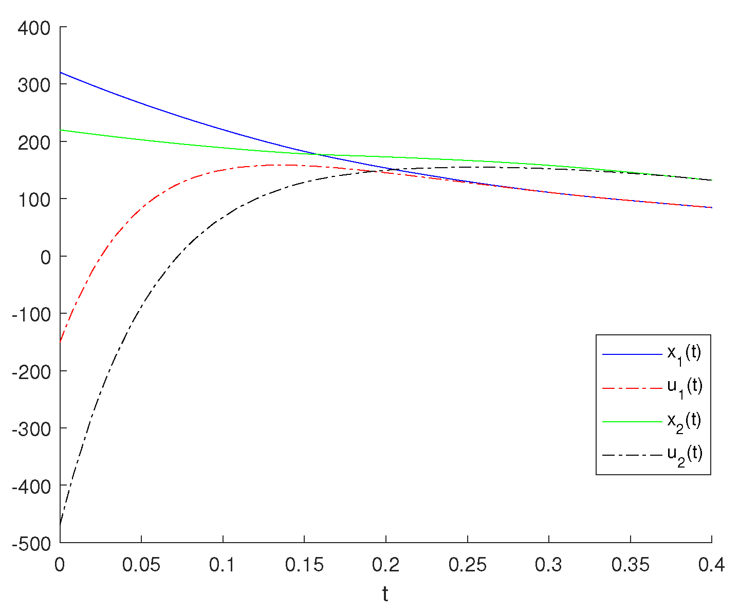
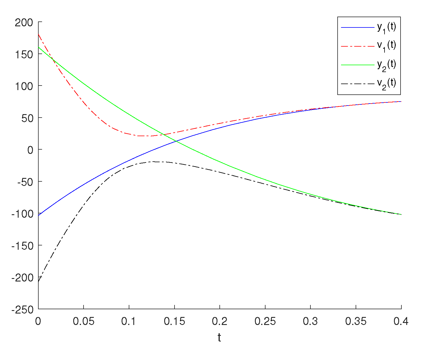
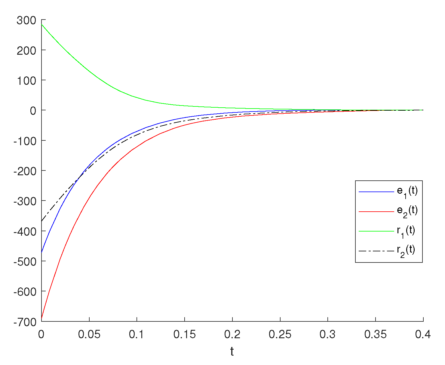
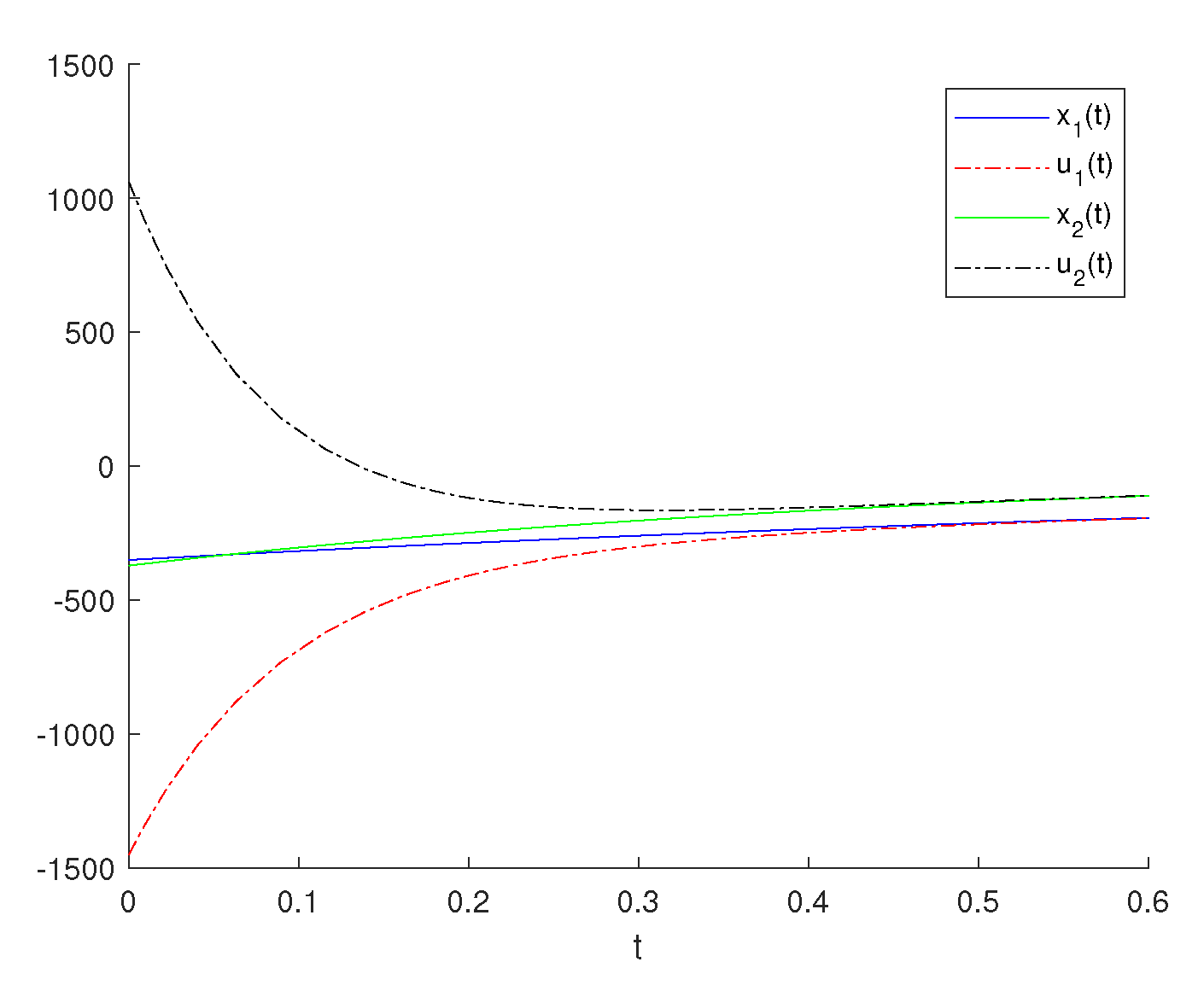
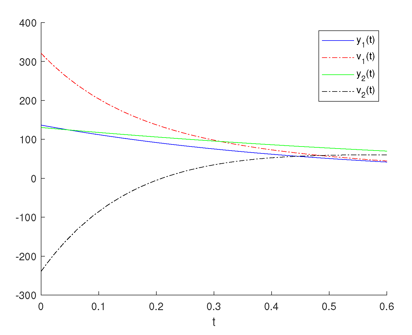
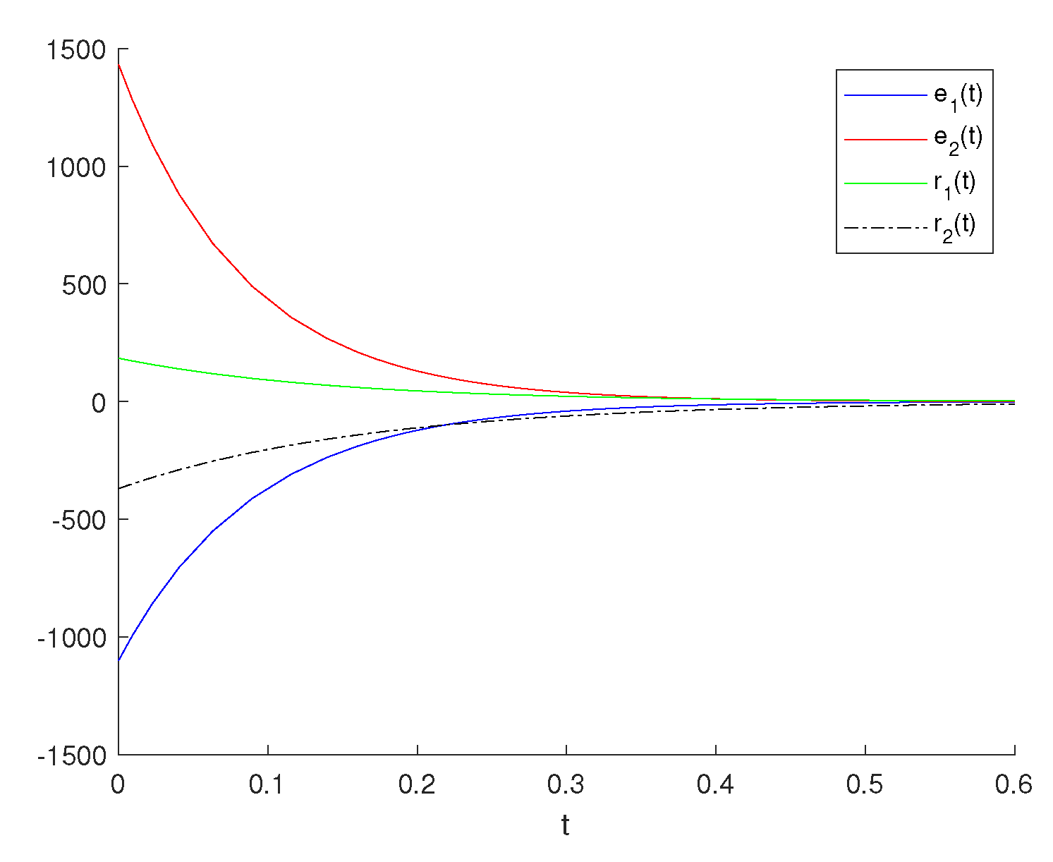
4. Numerical Examples

A BAM neural network composed of neurons arranged in two layers possesses good applications in the field of pattern recognition and artificial intelligence, since BAM neural networks have the capability to learn from a process. Hence, the study of synchronization in practical application for the drive–response BAM neural networks is very necessary. In this section, we give two examples to illustrate our theoretical results by intuitive images.

Example 1.

We consider system (1), response system (2) and error system (3) with controllers (4) for $i=1,2;$ $j=1,2$, where $c_{11}=3,$ $c_{12}=-2,$ $c_{21}=4,$ $c_{22}=-5;$ $d_{11}=1,$ $d_{12}=-4,$ $d_{21}=-2,$ $d_{22}=3;$ $p_{11}=-1,$ $p_{12}=3,$ $p_{21}=0.9,$ $p_{22}=-2;$ $q_{11}=4,$ $q_{12}=-3,$ $q_{21}=-5,$ $q_{22}=2.$ $a_1=3,$ $a_2=1,$ $b_1=4,$ $b_2=2,$ $p=2>1,$ $a=3>1,k_1=1>0,$ $k_2=-16<0,$ $k_3=-3<0,$ $l_1=2>0,$ $l_2=-8<0,$ $l_3=-5<0,$ $\varphi (t)=\frac{4}{4t+1}-{(t+\frac{1}{4})}^{a-1}-1,$ $I_1=1,$ $I_2=-2,$ $J_1=1,$ $J_2=2,$ $f_j(y_j(t))=0.5|y_j(t)|-1,g_i(x_i(t))=0.7|x_i(t)|+1,$ ${\tau }_{ji}(t)=0.5sint$ and ${\sigma }_{ij}(t)=0.5cost.$ The initial conditions are given as: $x_1(0)=320.5,x_2(0)=220,y_1(0)=-103.7,y_2(0)=160.4,u_1(0)=-150.8,u_2(0)=-470,v_1(0)=180.7,v_2(0)=-207.6$. Thus, we have $A_1=-19.07<0,A_2=-16.5<0,B_1=-9.8<0,B_2=-2.57<0$ and

$$p{k}_3+k_1^p{\left(\frac{p-1}{-A_1}\right)}^{p-1}=-5.9476<0,p{k}_3+k_1^p{\left(\frac{p-1}{-A_2}\right)}^{p-1}=-5.9394<0,$$

$$p{l}_3+l_1^p{\left(\frac{p-1}{-B_1}\right)}^{p-1}=-9.5918<0,p{l}_3+l_1^p{\left(\frac{p-1}{-B_2}\right)}^{p-1}=-8.4436<0.$$

The controllers from (4) for Example 1 are different from those in the literature [14,15,16,17,18,19,20,21,22,42]. It is not difficult to verify that the parameters do not satisfy the conditions of finite-time synchronization from the above papers. Therefore, the finite-time synchronization of the drive system (1) and response system (2) cannot be verified with the results in [14,15,16,17,18,19,20,21,22,42]. It is easy to verify that $(H_1)$–$(H_3)$ in Theorem 1 in our paper are satisfied. Hence, by Theorem 1 in our paper, the drive system (1) and the response system (2) are finite-time synchronized under controllers (4). The curves of variables $x_1(t),x_2(t),u_1(t)$ and $u_2(t)$ are shown in Figure 1, the curves of variables $y_1(t),y_2(t),v_1(t)$ and $v_2(t)$ are shown in Figure 2 and the error curves of the drive–response system $e_1(t),e_2(t),r_1(t)$ and $r_2(t)$ are shown in Figure 3.

Example 2.

We consider drive system (1), response system (2) and error system (3) with controllers (5) for $i=1,2;j=1,2$, where $c_{11}=0.3,$ $c_{12}=-0.2,$ $c_{21}=0.4,$ $c_{22}=-0.5;$ $d_{11}=0.6,$ $d_{12}=-0.4,$ $d_{21}=-0.2,$ $d_{22}=0.3;$ $p_{11}=-0.1,$ $p_{12}=0.6,$ $p_{21}=0.8,$ $p_{22}=-0.2;$ $q_{11}=0.8,$ $q_{12}=0.3,$ $q_{21}=0.5,$ $q_{22}=0.9.$ $a_1=1,$ $a_2=2,$ $b_1=2,$ $b_2=1,$ $q=2>1,$ $b=-5<-3,$ $w_1=1>0,$ $w_2=-10<0,$ $w_3=-3<0,$ $z_1=2>0,$ $z_2=-5<0,$ $z_3=-3<0,$ $\psi (t)=1+a^{*}-a^{*}(e^t+t{e}^t)-e^t-3M(0),t\ge \frac{1}{e},$ $a^{*}=10,$ $I_1=-1,$ $I_2=2,$ $J_1=3,$ $J_2=-2,$ $f_j(y_j)=0.5sin(y_j)+0.5,g_i(x_i)=0.25cos(x_i)-1,{\tau }_{ji}(t)=0.4cost$ and ${\sigma }_{ij}(t)=0.6sint.$ Furthermore, the initial conditions are defined as: $x_1(0)=-350.5,x_2(0)=-371.63,y_1(0)=136.48,y_2(0)=130.4,u_1(0)=-1450.8,u_2(0)=1060.63,v_1(0)=320.73$ and $v_2(0)=-238.82$. Hence, we have $C_1=-40.7125<0,C_2=-44.9500<0,D_1=-25.6333<0,D_2=-21.2667<0$ and

$$2q{w}_3+2^q{w}_1^q{\left(\frac{q-1}{-C_1}\right)}^{q-1}=-11.9996<0,2q{w}_3+2^q{w}_1^q{\left(\frac{q-1}{-C_2}\right)}^{q-1}=-11.9997<0,$$

$$2q{z}_3+2^q{z}_1^q{\left(\frac{q-1}{-D_1}\right)}^{q-1}=-11.9744<0,2q{z}_3+2^q{z}_1^q{\left(\frac{q-1}{-D_2}\right)}^{q-1}=-11.9551<0.$$

The controllers from (5), are different from those in [14,15,16,17,18,19,20,21,22,42]. We can easily verify that the parameters do not satisfy the conditions on finite-time synchronization from the above literature. Hence, the finite-time synchronization of drive system (1) and response system (2) cannot be verified with the results from [14,15,16,17,18,19,20,21,22,42]. We can verify that $(H_1),(H_4)$ and $(H_5)$ are satisfied. As a result, by Theorem 2, the drive system (1) and the response system (2) are finite-time synchronized under controllers (5).

The curves of variables $x_1(t),x_2(t),u_1(t)$ and $u_2(t)$ are shown in Figure 4, the curves of variables $y_1(t),y_2(t),v_1(t)$ and $v_2(t)$ are shown in Figure 5 and the error curves of the drive–response system $e_1(t),e_2(t),r_1(t)$ and $r_2(t)$ are shown in Figure 6.

5. Conclusions

In this paper, we focused on the finite-time synchronization for a class of drive–response BAM neural networks with time-varying delays. Furthermore, two novel finite-time synchronization conditions of the above BAM neural networks were derived to assure the finite-time synchronization between the drive system and the response system. In that process, we applied the maximum-value approach and introduced two new inequalities, which were different from those in the existing papers. In the future, we will study the fixed-time synchronization of neural networks.

References

1. Kosko, B. Adaptive bidirectional associative memories. Appl. Opt. 1987, 26, 4947–4960. [Google Scholar] [CrossRef] [PubMed] [Green Version]
2. Kosko, B. Bidirectional associative memories. IEEE Trans. Syst. Man Cybern. 1988, 18, 49–60. [Google Scholar] [CrossRef] [Green Version]
3. Shafiya, M.; Nagamani, G.; Dafik, D. Global synchronization of uncertain fractional-order BAM neural networks with time delay via improved fractional-order integral inequality. Math. Comput. Simul. 2021, 191, 168–186. [Google Scholar] [CrossRef]
4. Zhao, Y.; Ren, S.; Kurths, J. Synchronization of coupled memristive competitive BAM neural networks with different time scales. Neurocomputing 2021, 427, 110–117. [Google Scholar] [CrossRef]
5. Xiao, J.; Zhong, S.; Wen, S. Improved approach to the problem of the global Mittag–Leffler synchronization for fractional-order multidimension-valued BAM neural networks based on new inequalities. Neural Netw. 2021, 133, 87–100. [Google Scholar] [CrossRef]
6. Lin, F.; Zhang, Z. Global asymptotic synchronization of a class of BAM neural networks with time delays via integrating inequality techniques. J. Syst. Sci. Complex. 2020, 33, 366–382. [Google Scholar] [CrossRef]
7. Xiao, J.; Wen, S.; Yang, X.; Zhong, S. New approach to global Mittag–Leffler synchronization problem of fractional-order quaternion-valued BAM neural networks based on a new inequality. Neural Netw. 2020, 122, 320–337. [Google Scholar] [CrossRef]
8. Zhang, J.; Wu, J.; Bao, H.; Cao, J. Synchronization analysis of fractional-order three-neuron BAM neural networks with multiple time delays. Appl. Math. Comput. 2018, 339, 441–450. [Google Scholar] [CrossRef]
9. Wang, D.; Huang, L.; Tang, L. Dissipativity and synchronization of generalized BAM neural networks with multivariate discontinuous activations. IEEE Trans. Neural Netw. Learn. Syst. 2018, 29, 3815–3827. [Google Scholar]
10. Ye, R.; Liu, X.; Zhang, H.; Cao, J. Global Mittag–Leffler synchronization for fractional-order BAM neural networks with impulses and multiple variable delays via delayed-feedback control strategy. Neural Process. Lett. 2019, 49, 1–18. [Google Scholar] [CrossRef]
11. Zhang, Z.; Li, A.; Yang, L. Global asymptotic periodic synchronization for delayed complex-valued BAM neural networks via vector-valued inequality techniques. Neural Process. Lett. 2018, 48, 1019–1041. [Google Scholar] [CrossRef]
12. Yang, W.; Yu, W.; Cao, J.; Alsaadi, F.E.; Hayat, T. Global exponential stability and lag synchronization for delayed memristive fuzzy Cohen-Grossberg BAM neural networks with impulses. Neural Netw. 2018, 98, 122–153. [Google Scholar] [CrossRef] [PubMed]
13. Wang, W.; Yu, M.; Luo, X.; Liu, L.; Yuan, M.; Zhao, W. Synchronization of memristive BAM neural networks with leakage delay and additive time-varying delay components via sampled-data control. Chaos Solitons Fractals 2017, 104, 84–97. [Google Scholar] [CrossRef]
14. Zhou, Z.; Zhang, Z.; Chen, M. Finite-time synchronization for fuzzy delayed neutral-type inertial Bam neural networks via the figure analysis approach. Int. J. Fuzzy Syst. 2022, 24, 229–246. [Google Scholar] [CrossRef]
15. Li, L.; Xu, R.; Gan, Q.; Lin, J. A switching control for finite-time synchronization of memristor-based BAM neural networks with stochastic disturbances. Nonlinear Anal. Model. Control 2020, 25, 958–979. [Google Scholar] [CrossRef]
16. Du, F.; Lu, J. New criterion for finite-time synchronization of fractional order memristor-based neural networks with time delay. Appl. Math. Comput. 2021, 389, 125616. [Google Scholar] [CrossRef]
17. Zhang, L.; Yang, Y. Finite time impulsive synchronization of fractional order memristive BAM neural networks. Neurocomputing 2020, 384, 213–224. [Google Scholar] [CrossRef]
18. Tang, R.; Yang, X.; Wan, X.; Zou, Y.; Cheng, Z.; Fardoun, H.M. Finite-time synchronization of nonidentical BAM discontinuous fuzzy neural networks with delays and impulsive effects via non-chattering quantized control. Commun. Nonlinear Sci. Numer. Simul. 2019, 78, 104893. [Google Scholar] [CrossRef]
19. Wang, W.; Wang, X.; Luo, X.; Yuan, M. Finite-time projective synchronization of memristor-based BAM neural networks and applications in image encryption. IEEE Access 2018, 6, 56457–56476. [Google Scholar] [CrossRef]
20. Zhang, Y.; Li, L.; Peng, H.; Xiao, J.; Yang, Y.; Zheng, M.; Zhao, H. Finite-time synchronization for memristor-based BAM neural networks with stochastic perturbations and time-varying delays. Int. J. Robust Nonlinear Control 2018, 28, 5118–5139. [Google Scholar] [CrossRef]
21. Guo, R.; Zhang, Z.; Chen, J.; Lin, C.; Liu, Y. Finite-time synchronization for delayed complex-valued BAM neural networks. In Proceedings of the 2017 Chinese Automation Congress (CAC), Jinan, China, 20–22 October 2017; pp. 872–877. [Google Scholar]
22. Xiao, J.; Zhong, S.; Li, Y.; Xu, F. Finite-time Mittag–Leffler synchronization of fractional-order memristive BAM neural networks with time delays. Neurocomputing 2017, 219, 431–439. [Google Scholar] [CrossRef]
23. Chen, S.; Li, H.; Kao, Y.; Zhang, L.; Hu, C. Finite-time stabilization of fractional-order fuzzy quaternion-valued BAM neural networks via direct quaternion approach. J. Frankl. Inst. 2021, 358, 7650–7673. [Google Scholar] [CrossRef]
24. Cao, Y.; Ramajayam, S.; Sriraman, R.; Samidurai, R. Leakage delay on stabilization of finite-time complex-valued BAM neural network: Decomposition approach. Neurocomputing 2021, 463, 505–513. [Google Scholar] [CrossRef]
25. Yan, H.; Qiao, Y.; Duan, L.; Zhang, L. Global Mittag–Leffler stabilization of fractional-order BAM neural networks with linear state feedback controllers. Math. Probl. Eng. 2020, 2020, 6398208. [Google Scholar] [CrossRef]
26. Arslan, E.; Narayanan, G.; Ali, M.S.; Arik, S.; Saroha, S. Controller design for finite-time and fixed-time stabilization of fractional-order memristive complex-valued BAM neural networks with uncertain parameters and time-varying delays. Neural Netw. 2020, 130, 60–74. [Google Scholar] [CrossRef]
27. Cong, E.; Han, X.; Zhang, X. New stabilization method for delayed discrete-time Cohen-Grossberg BAM neural networks. IEEE Access 2020, 8, 99327–99336. [Google Scholar] [CrossRef]
28. Pratap, A.; Raja, R.; Cao, J.; Rihan, F.A.; Seadawy, A.R. Quasi-pinning synchronization and stabilization of fractional order BAM neural networks with delays and discontinuous neuron activations. Chaos Solitons Fractals 2020, 131, 109491. [Google Scholar] [CrossRef]
29. Yang, Z.; Li, J.; Niu, Y. Finite-time stabilization of fractional-order delayed bidirectional associative memory neural networks. Sci. Asia 2019, 45, 589–596. [Google Scholar] [CrossRef] [Green Version]
30. Yang, Z.; Zhang, J. Global stabilization of fractional-order bidirectional associative memory neural networks with mixed time delays via adaptive feedback control. Int. J. Comput. Math. 2020, 97, 2074–2090. [Google Scholar] [CrossRef]
31. Cheng, W.; Wu, A.; Zhang, J.; Li, B. Adaptive control of Mittag–Leffler stabilization and synchronization for delayed fractional-order BAM neural networks. Adv. Differ. Equ. 2019, 2019, 337. [Google Scholar] [CrossRef] [Green Version]
32. Lu, B.; Jiang, H.; Hu, C.; Abdurahman, A. Pinning impulsive stabilization for BAM reaction-diffusion neural networks with mixed delays. J. Frankl. Inst. 2018, 355, 8802–8829. [Google Scholar] [CrossRef]
33. Chinnathambi, R.; Rihan, F.A.; Shanmugam, L. Stabilization of delayed Cohen-Grossberg BAM neural networks. Math. Methods Appl. Sci. 2018, 41, 593–605. [Google Scholar] [CrossRef]
34. Guo, R.; Zhang, Z.; Liu, X.; Lin, C. Existence, uniqueness, and exponential stability analysis for complex-value d memristor-base d BAM neural networks with time delays. Appl. Math. Comput. 2017, 311, 100–117. [Google Scholar]
35. Zhang, Z.; Liu, X.; Guo, R.; Lin, C. Finite-time stability for delayed complex-valued BAM neural networks. Neural Process. Lett. 2018, 48, 179–193. [Google Scholar] [CrossRef]
36. Gunasekaran, N.; Syed Ali, M. Design of stochastic passivity and passification for delayed BAM neural networks with Markov jump parameters via non-uniform sampled-data control. Neural Process. Lett. 2021, 53, 391–404. [Google Scholar] [CrossRef]
37. Yan, M.; Jian, J.; Zheng, S. Passivity analysis for uncertain BAM inertial neural networks with time-varying delays. Neurocomputing 2021, 435, 114–125. [Google Scholar] [CrossRef]
38. Xing, L.; Zhou, L. Polynomial dissipativity of proportional delayed BAM neural networks. Int. J. Biomath. 2020, 13, 2050050. [Google Scholar] [CrossRef]
39. Chandran, S.; Ramachandran, R.; Cao, J.; Agarwal, R.P.; Rajchakit, G. Passivity analysis for uncertain BAM neural networks with leakage, discrete and distributed delays using novel summation inequality. Int. J. Control. Autom. Syst. 2019, 17, 2114–2124. [Google Scholar] [CrossRef]
40. Saravanakumar, R.; Rajchakit, G.; Ali, M.S.; Joo, Y.H. Exponential dissipativity criteria for generalized BAM neural networks with variable delays. Neural Comput. Appl. 2019, 31, 2717–2726. [Google Scholar] [CrossRef]
41. Sowmiya, C.; Raja, R.; Cao, J.; Rajchakit, G.; Alsaedi, A. Enhanced robust finite-time passivity for Markovian jumping discrete-time BAM neural networks with leakage delay. Adv. Differ. Equ. 2017, 2017, 318. [Google Scholar] [CrossRef] [Green Version]
42. Zhang, Z.; Cao, J. Finite-time synchronization for fuzzy inertial neural networks by maximum-value approach. IEEE Trans. Fuzzy Syst. 2021. [Google Scholar] [CrossRef]
43. Wang, Z.; He, H. Asynchronous quasi-consensus of heterogeneous multiagent systems with nonuniform input delays. IEEE Trans. Syst. Man Cybern. Syst. 2020, 50, 2815–2827. [Google Scholar] [CrossRef]
44. Wang, Z.; Jin, X.; Pan, L.; Feng, Y.; Cao, J. Quasi-synchronization of delayed stochastic multiplex networks via impulsive pinning control. IEEE Trans. Syst. Man Cybern. Syst. 2021, 1–9. [Google Scholar] [CrossRef]
45. Wang, Z.; He, H.; Jiang, G.-P.; Cao, J. Quasi-Synchronization in heterogeneous harmonic oscillators with continuous and sampled coupling. IEEE Trans. Syst. Man Cybern. Syst. 2021, 51, 1267–1277. [Google Scholar] [CrossRef]
46. Saker, S.; Kenawy, M.; AlNemer, G.; Zakarya, M. Some fractional dynamic inequalities of Hardy’s type via conformable calculus. Mathematics 2020, 8, 434. [Google Scholar] [CrossRef] [Green Version]
47. Anbuvithya, R.; Mathiyalagan, K.; Sakthivel, R.; Prakash, P. Non-fragile synchronization of memristive BAM networks with random feedback gain fluctuations. Commun. Nonlinear Sci. Numer. Simul. 2015, 29, 427–440. [Google Scholar] [CrossRef]
48. Zhang, Z.; Cao, J. Novel finite-time synchronization criteria for inertial neural networks with time delays via integral inequality method. IEEE Trans. Neural Netw. Learn. Syst. 2019, 30, 1476–1484. [Google Scholar] [CrossRef]
49. Zhang, Z.; Li, A.; Hua, S. Finite-time synchronization for delayed complex-valued neural networks via integrating inequality method. Neurocomputing 2018, 318, 248–260. [Google Scholar] [CrossRef]
50. Zhang, Z.; Chen, M.; Li, A. Further study on finite-time synchronization for delayed inertial neural networks via inequality skills. Neurocomputing 2020, 373, 15–23. [Google Scholar] [CrossRef]
51. Kuang, J. Applied Inequalities, 3rd ed.; Shandong Science and Technology Press: Jinan, China, 2004. [Google Scholar]
Figure 1. The curves of x 1 ( t ) , x 2 ( t ) , u 1 ( t ) , u 2 ( t ) from Example 1.
Mathematics 10 00835 g001
Figure 2. The curves of y 1 ( t ) , y 2 ( t ) , v 1 ( t ) , v 2 ( t ) from Example 1.
Mathematics 10 00835 g002
Figure 3. The curves of e 1 ( t ) , e 2 ( t ) , r 1 ( t ) , r 2 ( t ) from Example 1.
Mathematics 10 00835 g003
Figure 4. The curves of x 1 ( t ) , x 2 ( t ) , u 1 ( t ) , u 2 ( t ) from Example 2.
Mathematics 10 00835 g004
Figure 5. The curves of y 1 ( t ) , y 2 ( t ) , v 1 ( t ) , v 2 ( t ) from Example 2.
Mathematics 10 00835 g005
Figure 6. The curves of e 1 ( t ) , e 2 ( t ) , r 1 ( t ) , r 2 ( t ) from Example 2.
Mathematics 10 00835 g006
Publisher’s Note: MDPI stays neutral with regard to jurisdictional claims in published maps and institutional affiliations.