A Simple, Accurate and Semi-Analytical Meshless Method for Solving Laplace and Helmholtz Equations in Complex Two-Dimensional Geometries

Abstract

A localized virtual boundary element–meshless collocation method (LVBE-MCM) is proposed to solve Laplace and Helmholtz equations in complex two-dimensional (2D) geometries. “Localized” refers to employing the moving least square method to locally approximate the physical quantities of the computational domain after introducing the traditional virtual boundary element method. The LVBE-MCM is a semi-analytical and domain-type meshless collocation method that is based on the fundamental solution of the governing equation, which is different from the traditional virtual boundary element method. When it comes to 2D problems, the LVBE-MCM only needs to calculate the numerical integration on the circular virtual boundary. It avoids the evaluation of singular/strong singular/hypersingular integrals seen in the boundary element method. Compared to the difficulty of selecting the virtual boundary and evaluating singular integrals, the LVBE-MCM is simple and straightforward. Numerical experiments, including irregular and doubly connected domains, demonstrate that the LVBE-MCM is accurate, stable, and convergent for solving both Laplace and Helmholtz equations.

1. Introduction

The boundary element method (BEM) [1,2] is a well-known numerical method that has become an alternative to domain methods such as the finite element method (FEM) [3,4] for the simulation of certain physical problems. The core of this method is to accurately solve singular integrals, especially nearly singular, strongly singular, and hypersingular integrals, among others. Substantial efforts have been devoted to developing and applying efficient estimation techniques for such integrals. Lutz [5] proposed a special Gaussian-type numerical integral to calculate the singular and nearly singular integrals. Johnston and Elliott [6] proposed a sinh transformation to evaluate nearly singular integrals. Niu and Zhou [7,8] suggested that the asymptotic expansion of the kernel function with respect to the local co-ordinates should be employed to address singular integrals. Besides these methods, there are other techniques that can be used to deal with various singular integrals. Although they were proven to be the effective strategies, these methods are often time consuming, tedious, and expensive.

In recent years, the virtual boundary element method (VBEM) [9,10,11,12,13] has been proposed to overcome the above shortcomings. The VBEM introduces the virtual boundary to avoid the calculation of singular integrals and inherits the semi-analytical and high-accuracy features of the BEM. Sun and Yao [14] used the VBEM to successfully solve thin plate elastic obstacle problems. Yao et al. [10,15] used the VBEM to simulate magnetoelectroelastic and piezoelectric problems. Yang et al. [16] and Liu et al. [17] resolved three-dimensional inverse heat conduction problems using the VBEM. As a boundary-type scheme with global discretization, however, the VBEM encounters challenges when simulating large-scale and/or high-dimensional problems.

More recently, the localization of boundary-type meshless methods have received considerable attention, and various localized meshless methods [18,19,20,21,22,23] have been proposed to solve mathematical and mechanical problems, such as the generalized finite difference method (GFDM) [24,25], the localized method of fundamental solutions (LMFS) [26,27], the local knot method (LKM) [28,29], and the localized singular boundary method (LSBM) [30,31]. Unlike traditional boundary-type methods, these methods are not only simple, accurate, and easy-to-program, but also suitable for large-scale simulations in complicated domains. On the other hand, boundary-type meshless methods encounter many difficult issues. Similar to the fundamental solution method, the VBEM uses fundamental solutions as the basis functions and requires a virtual boundary outside of the physical domain to avoid source singularity. The selection of this artificial boundary is still a well-known tricky issue in spite of the great deal of effort that has been made to address this problem [32,33], especially in terms of complex geometries.

Motivated by the above works using localized methods, we establish a localized numerical framework for the VBEM in this paper, which we called the localized virtual boundary element–meshless collocation method (LVBE-MCM). The accuracy and effectiveness of the LVBE-MCM was verified via its ability to solve Laplace and Helmholtz equations in complex 2D domains. In the traditional VBEM, it is difficult to determine the position and shape of virtual boundaries in the complex domain because these boundaries have a certain impact on the calculation accuracy. On the contrary, the LVBE-MCM only uses the circular virtual boundary during the local approximation, and it is insensitive to the location of the boundary. Furthermore, the resulting LVBE-MCM system is sparse and can thus be easily solved using an ordinary computer. This also means that the method has certain application prospects for solving large-scale problems.

The rest of the paper is organized as follows: In Section 2, the considered problem is briefly introduced. Section 3 describes the detailed numerical procedure for the LVBE-MCM. Section 4 develops an augmented moving least squares approximation using the fundamental solutions. In Section 5, two numerical examples are provided to confirm the effectiveness and applicability of the proposed method. The conclusions are summarized in Section 6.

2. Preliminaries

Let $\Omega \in R^2$ be an open bounded domain surrounded by the boundary $\Gamma =\partial \Omega$, which is assumed to be piecewise smooth, and consider the following boundary value problem:

$$Lu(x)=0,\hspace{1em}x\in \Omega ,$$

(1)

$$u(x)=f(x),\hspace{1em}x\in {\Gamma }_D,$$

(2)

$$\frac{\partial u(x)}{\partial \mathrm{n}}=g(x),\hspace{1em}x\in {\Gamma }_N,$$

(3)

$$\alpha u(x)+\beta \frac{\partial u(x)}{\partial \mathrm{n}}=h(x),\hspace{1em}x\in {\Gamma }_R,$$

(4)

where $L$ is the Laplace ($L={\nabla }^2$) or Helmholtz ($L={\nabla }^2+{\lambda }^2$) operator, $\lambda$ is the wave number, $\mathrm{n}$ is the unit outward normal vector, $\alpha$ and $\beta$ are constants, and $f(x), g(x), h(x)$ are the provided smooth functions on the boundaries. Here, ${\Gamma }_D$, ${\Gamma }_N$, and ${\Gamma }_R$ represent the Dirichlet, Neumann, and Robin boundaries, respectively.

The fundamental solutions for the Laplace and Helmholtz operators are determined by [34]

$$u^{*}(r)=-\frac{1}{2\pi }\ln \left(r\right), \mathrm{for} \mathrm{Laplace} \mathrm{operator}$$

(5)

$$u^{*}(r)=\frac{\mathrm{i}}{4}{H}_0^{(1)}\left(\lambda r\right), \mathrm{for} \mathrm{Helmholtz} \mathrm{operator}$$

(6)

where $r$ denotes the Euclidean distance between the field point and the source point, and $H_0^{(1)}$ is a zero-order Hankel function of the first kind.

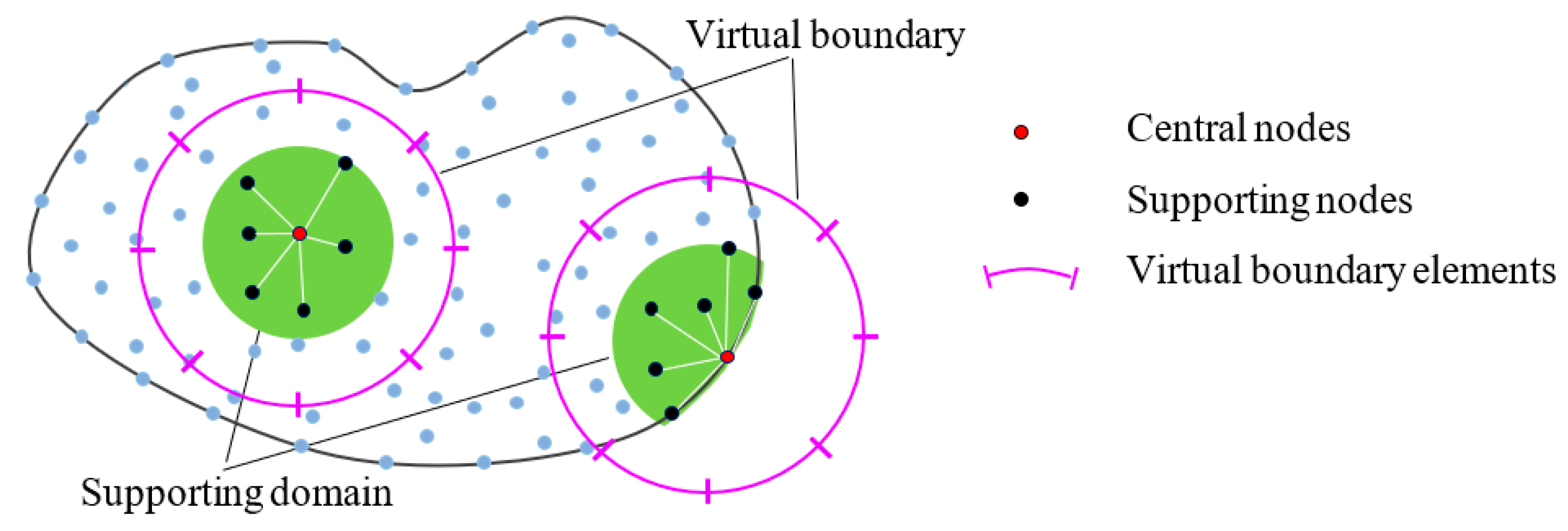
3. Localized Virtual Boundary Element–Meshless Collocation Method

First of all, the $N=n_i+n_{b1}+n_{b2}+n_{b3}$ discrete nodes $x_{}^{(i)}, i=1,2,\dots ,N$ are placed over the computational domain Ω, where n_i is the number of nodes inside the domain, and $n_{b1}$, $n_{b2}$, and $n_{b3}$ indicate the number of nodes along the Dirichlet, Neumann, and Robin boundary, respectively. Considering an arbitrary node $x^{(i)}$, which is also known as the central node, its m supporting nodes $x_j^{(i)}, j=1,2,\dots ,m$ can be determined based on the nearest nodes. At the same time, the local supporting domain ${\Omega }_s$ covering m+1 nodes can also be determined, and its virtual boundary ${\Gamma }^{(i)}$ can be specified at a certain distance from the boundary of the supporting domain. For 2D problems, this boundary is a circle. Figure 1 shows the schematic diagram of the LVBE-MCM.

In the present study, the virtual boundary is discretized by $M$ exact geometrical elements, and the physical quantity is approximated by the constant element. Using $x_0^{(i)}$ to represent $x_{}^{(i)}$, the unknowns at nodes $x_j^{(i)}, j=0,1,\dots ,m$ are expressed as

$$u\left(x_j^{(i)}\right)={\displaystyle {\int }_{{\Gamma }_{}^{(i)}}^{}{u}^{*}(x_j^{(i)},\xi ){\phi }^{(i)}(\xi )}d{\Gamma }_s^{(i)}={\displaystyle \sum _{k=1}^M{\phi }_k^{(i)}{\displaystyle {\int }_{{\Gamma }_k^{(i)}}^{}{u}^{*}(x_j^{(i)},\xi )}d{\Gamma }_k^{(i)}},\hspace{1em}{x}_j^{(i)}\in {\Omega }_s^{(i)},\hspace{1em}j=0,1,\dots ,m,$$

(7)

where $u^{*}(x_j^{(i)},\xi )$ is the fundamental solution of the governing equation, and $\phi (\xi )$ is the distribution density function associated with the virtual boundary ${\Gamma }_{}^{(i)}$. Equation (7) can be rewritten in the following matrix form:

$$u^{\left(i\right)}=G^{(i)}{\phi }^{(i)}.$$

(8)

For the above local approximation, the moving least squares (MLS) can be employed to obtain the unknown coefficient vector ${\phi }^{(i)}=\left[{\phi }_1^{(i)},{\phi }_2^{(i)},\dots ,{\phi }_M^{(i)}\right]$, resulting in

$${\phi }^{(i)}=H^{(i)}{u}^{(i)}.$$

(9)

Replacing $x_j^{(i)}$ in Equation (7) with $x_{}^{(i)}$, the following formula is yielded:

$$u\left(x_{}^{(i)}\right)={\displaystyle \sum _{k=1}^M{\phi }_k^{(i)}{\displaystyle {\int }_{{\Gamma }_k^{(i)}}^{}{u}^{*}(x_{}^{(i)},\xi )}d{\Gamma }_k^{(i)}}=E^{(i)}{\phi }^{(i)}.$$

(10)

Then, substituting Equation (9) into Equation (10), we obtain

$$u\left(x_{}^{(i)}\right)=E^{(i)}{H}^{(i)}{u}^{(i)}=F^{(i)}{u}^{\left(i\right)}.$$

(11)

If $x^{(i)}$ is a node on the boundary, the normal derivative can be calculated by

$$\frac{\partial u(x^{(i)})}{\partial n}=N^{(i)}{\phi }^{(i)}=N^{(i)}{H}^{(i)}{u}^{(i)}=C^{(i)}{u}^{\left(i\right)},$$

(12)

where $N^{(i)}=n_1{\sigma }_1^{(i)}+\dots +n_d{\sigma }_d^{(i)}$, and

$${\sigma }_l^{(i)}=\left[{\displaystyle {\int }_{{\Gamma }_1^{(i)}}\frac{\partial u^{*}(x^{(i)},\xi )}{\partial x_l^{(i)}}}d{\Gamma }_1^{(i)}, {\displaystyle {\int }_{{\Gamma }_2^{(i)}}\frac{\partial u^{*}(x^{(i)},\xi )}{\partial x_l^{(i)}}}d{\Gamma }_2^{(i)}, \dots ,\hspace{1em}{\displaystyle {\int }_{{\Gamma }_M^{(i)}}\frac{\partial u^{*}(x^{(i)},\xi )}{\partial x_l^{(i)}}}d{\Gamma }_M^{(i)}\right], l=1,\dots ,d.$$

(13)

In the above equations, $n_1,\dots ,n_d$ denote the components of the vector $n$, and $x_1^{(i)},\dots ,x_d^{(i)}$ denote the coordinate components of the node $x^{(i)}$.

Taking all of the nodes $x_{}^{(i)}, i=1,2,\dots ,N$ and the boundary data provided in Equations (2)–(4) into account, the following overdetermined equations can be obtained:

$$\{\begin{array}{l}{u}_i-F^{(i)}{u}^{\left(i\right)}=0,\hspace{1em}i\in \left\{1,2,\dots ,n_i\right\}\hfill \\ u_i=f_i,\hspace{1em}i\in \left\{n_i+1,\dots ,n_i+n_{b1}\right\}\hfill \\ E^{(i)}{u}^{(i)}=g_i,\hspace{1em}i\in \left\{n_i+n_{b1}+1,\dots ,n_i+n_{b1}+n_{b2}\right\}\hfill \\ \alpha u_i+E^{(i)}{u}^{(i)}=0,\hspace{1em}i\in \left\{n_i+n_{b1}+n_{b2}+1,\dots ,N\right\}\hfill \end{array}\mathrm{or} Au=b,$$

(14)

where $u={\left[u(x^{(1)}), u(x^{(2)}), \dots , u(x^{(N)})\right]}^T$, $b_{N\times 1}$ is a vector composed of zero elements and boundary data, and $A_{N\times N}$ is a sparse matrix. Equation (14) is a well-conditioned system, and in this work, it is solved by MATLAB routine “A\b”.

4. Augmented Moving Least Squares Approximation

The moving least squares approximation is a widely used technique in various meshless/meshfree methods. In this study, the fundamental solutions are introduced into the traditional moving least squares method, and we then developed the augmented moving least squares approximation, which is similar to the one outlined in [35]. According to its basic idea, the vector ${\alpha }^{(i)}$ is deduced by minimizing the following functional equation:

$$J{u}^{\left(i\right)}={\left(G^{\left(i\right)}{\phi }^{(i)}-u^{\left(i\right)}\right)}^{\mathrm{T}}{\omega }^{(i)}\left(G^{\left(i\right)}{\phi }^{(i)}-u^{\left(i\right)}\right),$$

(15)

where ${\omega }^{(i)}=diag\left(w_0^{(i)},w_1^{(i)},\dots ,w_m^{(i)}\right)$, and

$${\omega }_j^{(i)}=1-6{\left(d_j/d_{\max }\right)}^2+8{\left(d_j/d_{\max }\right)}^3-3{\left(d_j/d_{\max }\right)}^4,$$

(16)

in Equation (16), $d_j={\Vert x_j^{(i)}-x_{}^{(i)}\Vert }_2$ and $d_{\max }=\underset{j=0,1,\dots ,m}{\max }(d_j)$.

Hence, we have

$$\frac{\partial J{u}^{\left(i\right)}}{\partial {\phi }^{(i)}}=2{\left[G^{\left(i\right)}\right]}^T{\omega }^{(i)}{G}^{\left(i\right)}{\phi }^{(i)}-2{\left[G^{\left(i\right)}\right]}^T{\omega }^{(i)}{u}^{\left(i\right)}=0.$$

(17)

By calculating and reorganizing Equation (17), we can obtain a system equation in matrix form:

$$P^{(i)}{\phi }^{(i)}=Q^{(i)}{u}^{(i)},$$

(18)

where $P^{(i)}={\left[G^{\left(i\right)}\right]}^T{\omega }^{(i)}{G}^{\left(i\right)}$, and $Q^{(i)}={\left[G^{\left(i\right)}\right]}^T{\omega }^{(i)}$. Solving Equation (18) yields ${\phi }^{(i)}={\left[P^{(i)}\right]}^{-1}{Q}^{(i)}{u}^{(i)}$; hence, $H^{(i)}$ in Equation (9) is equal to ${\left[P^{(i)}\right]}^{-1}{Q}^{(i)}$. It should be pointed out that we used MATLAB’s mldivide (matrix left divide) function ($P^{(i)}\backslash Q^{(i)}$) to obtain $H^{(i)}$ instead of the matrix inversion.

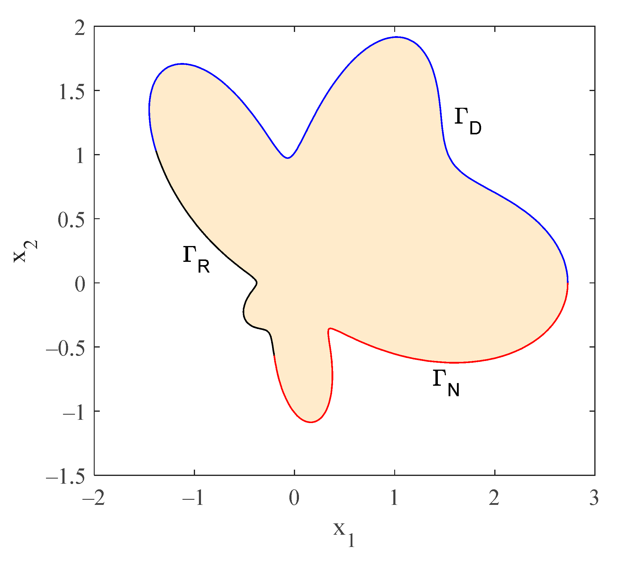
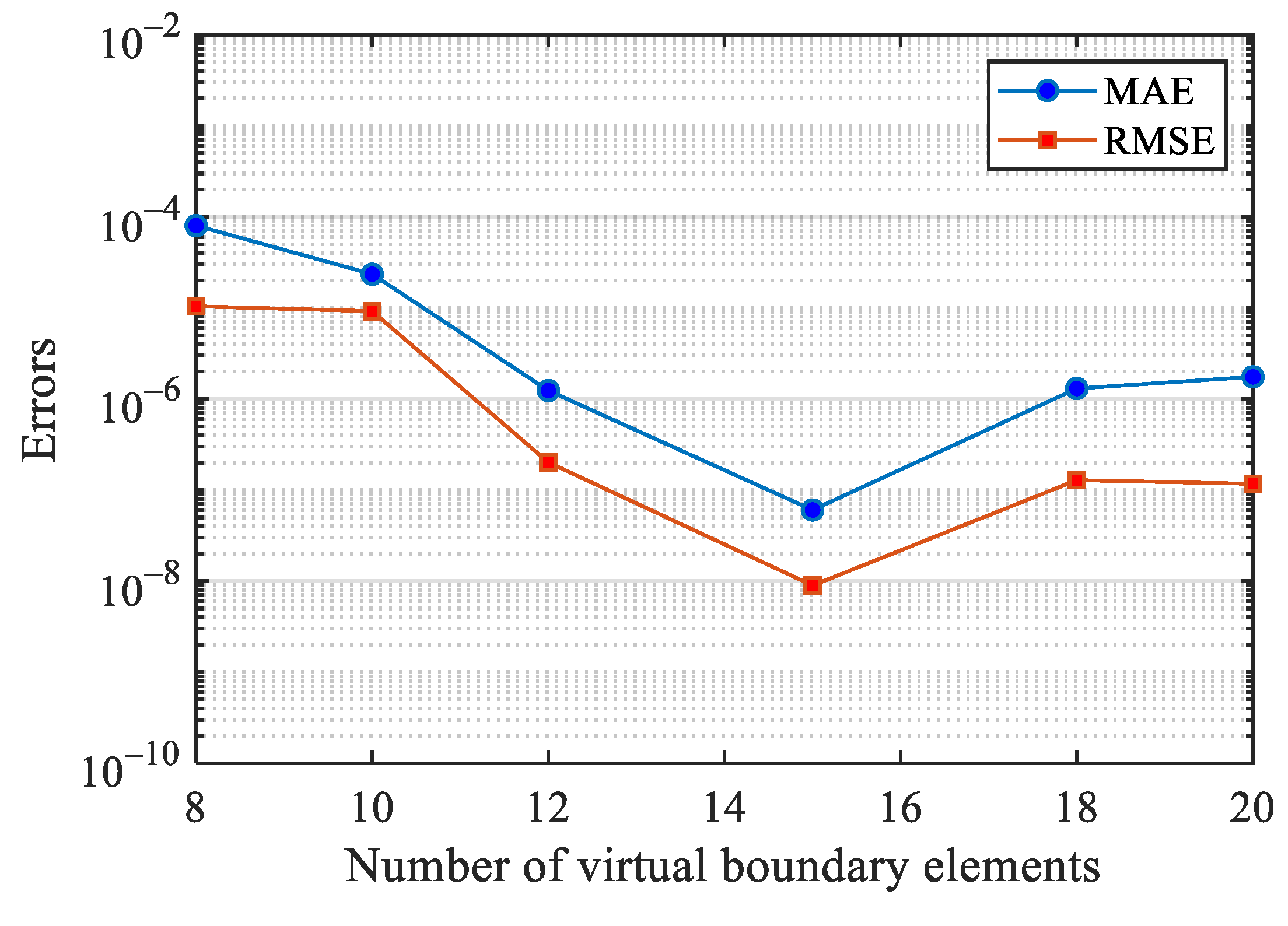
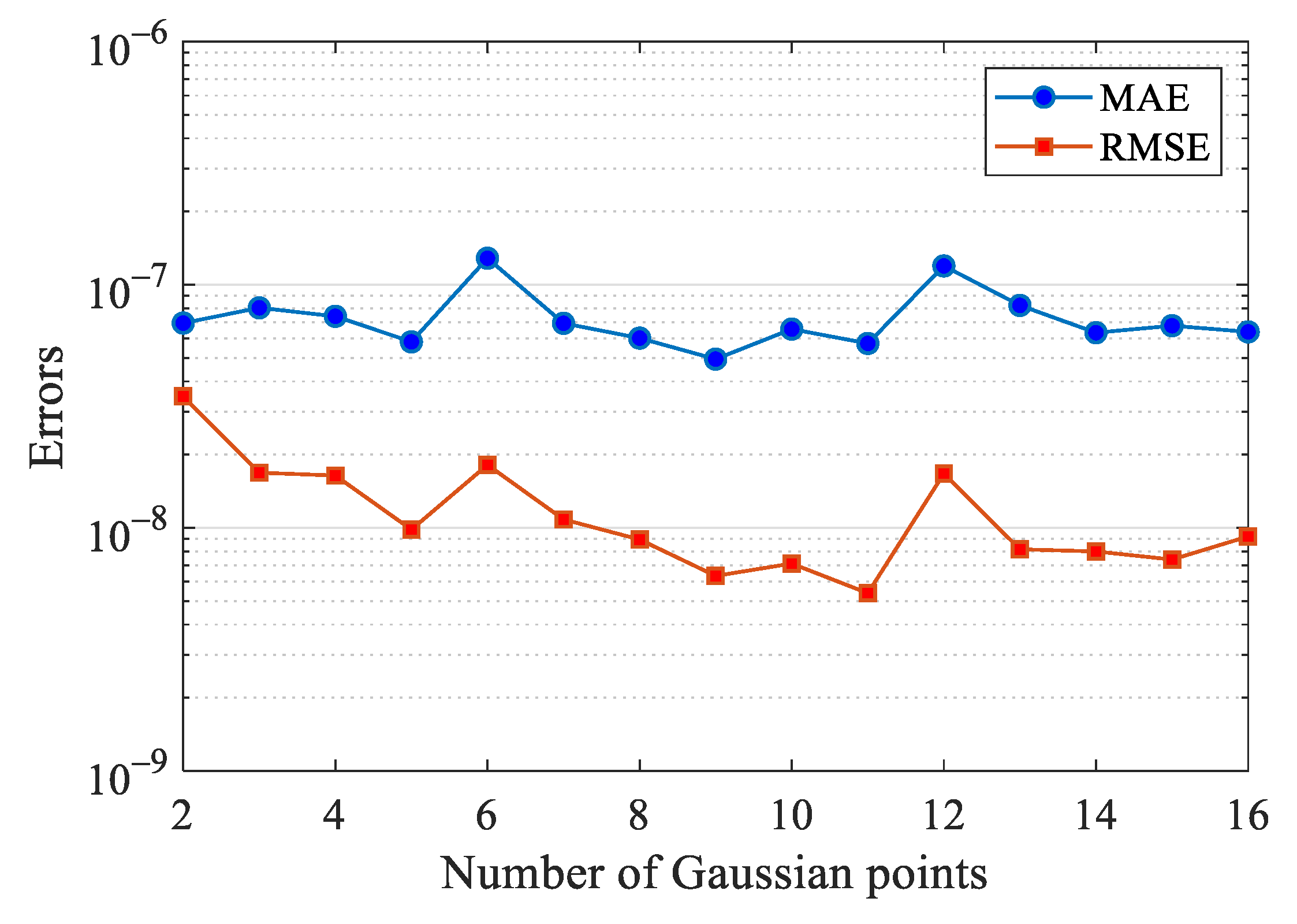
5. Numerical Examples

Two numerical examples are provided to demonstrate the effectiveness and accuracy of the proposed method. To evaluate the numerical errors, we adopt the maximum absolute error (MAE) and the root-mean-square error (RMSE), which are defined as follows:

$$\mathrm{MAE}=\underset{1\le j\le n_i}{\max }\left|u_n(x_j)-u_e(x_j)\right|,$$

(19)

$$\mathrm{RMSE}=\sqrt{\frac{1}{n_i}{\displaystyle \sum _{j=1}^{n_i}{(u_n(x_j)-u_e(x_j))}^2}},$$

(20)

where $u_n$ and $u_e$ represent the numerical and analytical solution at node $x_j$, respectively. All computations were performed using MATLAB 2018b on a desktop PC (Intel^® Core TMi7-6700 CPU at 3.4 GHz, 16G RAM, and Hard Disk-500G).

Example 1.

Consider a Laplace equation on an irregular domain with mixed boundary conditions. The geometry and boundary conditions are shown in Figure 2. For the Robin boundary condition, $\alpha =1$and $\beta =5$. The analytical solution is obtained by

$$u(x_1,x_2)=\cos (x_1)\cosh (x_2)+\sin (x_1)\sinh (x_2)+e^{x_1}\cos (x_2)+e^{x_2}\sin (x_1)+x_1{}^2-x_2{}^2+2x_1+3x_2+1.$$

(21)

First of all, N = 6784 nodes are chosen, and 8 Gaussian points are used. It can be seen from Figure 3 that the numerical error first decreases and then increases as the number of virtual elements increases, meaning that high computational accuracy has been achieved. Then, M = 15 is fixed. From Figure 4, we can observe that the number of Gaussian points has little effect on the calculation accuracy, and therefore, fewer Gaussian points can be used in the calculation.

The LMFS and GFDM are recently developed meshless approaches that are very similar to the present LVBE-MCM. In

Table 1. The RMSEs derived from the LVBE-MCM, LMFS, and GFDM under different numbers of total nodes.

N	448	765	1211	2592	4475	6784
LVBE-MCM	5.3674 × 10−7	3.7938 × 10−7	2.7616 × 10−7	1.2551 × 10−7	3.4856 × 10−8	8.9528 × 10−9
LMFS	1.4072 × 10−6	4.7048 × 10−7	4.3495 × 10−7	1.3170 × 10−7	1.4663 × 10−7	9.8769 × 10−8
GFDM	2.6038 × 10−3	4.2642 × 10−5	3.3704 × 10−5	1.6361 × 10−5	4.1832 × 10−7	1.3909 × 10−7

, these two methods are compared to the proposed approach. It can be observed that all methods are convergent. Although the LMFS and LVBE-MCM have similar numerical accuracy, the latter is slightly better than the former.

Example 2.

A Helmholtz equation on a doubly connected domain (see Figure 5) is considered. The boundary conditions are specified by the analytical solution$u(x_1,x_2)=\cos (x_1/2+\sqrt{3}{x}_2/2)$with$\lambda =1$.

The profiles of the exact solution and absolute error in the computational domain under N = 1840 and M = 15 are shown in Figure 6. The maximum absolute error and the root-mean-square error are 3.3238 × 10^–8 and 6.4048 × 10^–9, respectively. This indicates the high-accuracy of the proposed method. Furthermore, it can be observed from

Table 2. The RMSEs derived from the LVBE-MCM and LMFS under different elements or sources.

M	10	15	20	25	30	35
LVBE-MCM	3.6573 × 10−6	6.4048 × 10−9	1.1714 × 10−8	5.7849 × 10−8	5.1474 × 10−8	4.8111 × 10−8
LMFS	1.4772 × 10−5	1.3537 × 10−8	3.5835 × 10−8	7.4075 × 10−8	6.5249 × 10−8	6.7892 × 10−8

that the LVBE-MCM has higher numerical accuracy than the LMFS when the same number of sources and elements is adopted.

6. Conclusions

The localized virtual boundary element–meshless collocation method (LVBE-MCM) was proposed as a novel domain-type meshless method that could be used to solve Laplace and Helmholtz equations in complex 2D geometries. In this work, the traditional virtual boundary element method with a global approximation was modified to a local approximation approach by introducing the moving least square method and local approximation theory. Numerical integrations are only required on the circular virtual boundary; thus, the exact geometry elements are convenient to use. The proposed LVBE-MCM avoids the need to evaluate the singular/strong singular/hypersingular integral in the boundary element method and has a higher calculation accuracy than the LMFS.

Two examples involving irregular geometries and doubly connected domains were investigated in detail. The numerical results indicate that the LVBE-MCM is accurate and effective for solving Laplace and Helmholtz equations in complex two-dimensional geometries. The number of Gaussian points has a little effect on the calculation accuracy, and therefore, fewer Gaussian points can be used in the calculation. Moreover, the scheme is convergent with respect to increasing the number of total nodes. It is worth noting that the proposed method can be directly extended to other partial differential equations with known fundamental solutions, such as diffusion equations, Stokes equations, and biharmonic equations.

It should also be pointed out that this paper investigates the accuracy and convergence of the LVBE-MCM numerically. Unlike the difference method and Taylor expansion, it is not an easy work to formally prove the convergence and stability of the LVBE-MCM since there are few related assumptions and theorems on approximation techniques that use the fundamental solution and the augmented moving least squares scheme. Consequently, a theoretical analysis of the LVBE-MCM will be the key issue in our subsequent work.

References

1. Liu, Y.J.; Mukherjee, S.; Nishimura, N.; Schanz, M.; Ye, W.; Sutradhar, A.; Pan, E.; Dumont, N.A.; Frangi, A.; Saez, A. Recent Advances and Emerging Applications of the Boundary Element Method. Appl. Mech. Rev. 2011, 64, 030802. [Google Scholar] [CrossRef] [Green Version]
2. Beer, G.; Smith, I.; Duenser, C. The Boundary Element Method with Programming: For Engineers and Scientists; Springer: Vienna, Austria, 2008. [Google Scholar]
3. Chai, Y.; Li, W.; Liu, Z. Analysis of transient wave propagation dynamics using the enriched finite element method with interpolation cover functions. Appl. Math. Comput. 2022, 412, 126564. [Google Scholar] [CrossRef]
4. Li, W.; Zhang, Q.; Gui, Q.; Chai, Y. A Coupled FE-Meshfree Triangular Element for Acoustic Radiation Problems. Int. J. Comput. Methods 2021, 18, 2041002. [Google Scholar] [CrossRef]
5. Lutz, E. Exact Gaussian quadrature methods for near-singular integrals in the boundary element method. Eng. Anal. Bound. Elements 1992, 9, 233–245. [Google Scholar] [CrossRef]
6. Johnston, P.R.; Elliott, D. A sinh transformation for evaluating nearly singular boundary element integrals. Int. J. Numer. Methods Eng. 2005, 62, 564–578. [Google Scholar] [CrossRef]
7. Zhou, H.; Niu, Z.; Cheng, C.; Guan, Z. Analytical integral algorithm applied to boundary layer effect and thin body effect in BEM for anisotropic potential problems. Comput. Struct. 2008, 86, 1656–1671. [Google Scholar] [CrossRef]
8. Niu, Z.; Cheng, C.; Zhou, H.; Hu, Z. Analytic formulations for calculating nearly singular integrals in two-dimensional BEM. Eng. Anal. Bound. Elements 2007, 31, 949–964. [Google Scholar] [CrossRef]
9. Cascio, M.L.; Milazzo, A.; Benedetti, I. A hybrid virtual–boundary element formulation for heterogeneous materials. Int. J. Mech. Sci. 2021, 199, 106404. [Google Scholar] [CrossRef]
10. Yao, W.; Wang, H. Virtual boundary element integral method for 2-D piezoelectric media. Finite Elem. Anal. Des. 2005, 41, 875–891. [Google Scholar]
11. Lee, C. Stability characteristics of the virtual boundary method in three-dimensional applications. J. Comput. Phys. 2003, 184, 559–591. [Google Scholar] [CrossRef]
12. Saiki, E.; Biringen, S. Numerical Simulation of a Cylinder in Uniform Flow: Application of a Virtual Boundary Method. J. Comput. Phys. 1996, 123, 450–465. [Google Scholar] [CrossRef]
13. Desiderio, L.; Falletta, S.; Scuderi, L. A Virtual Element Method coupled with a Boundary Integral Non Reflecting condition for 2D exterior Helmholtz problems. Comput. Math. Appl. 2021, 84, 296–313. [Google Scholar] [CrossRef]
14. Huanchun, S.; Weian, Y. Virtual boundary element-linear complementary equations for solving the elastic obstacle problems of thin plate. Finite Elements Anal. Des. 1997, 27, 153–161. [Google Scholar] [CrossRef]
15. Li, X.-C.; Yao, W.-A. Virtual boundary element-integral collocation method for the plane magnetoelectroelastic solids. Eng. Anal. Bound. Elem. 2006, 30, 709–717. [Google Scholar] [CrossRef]
16. Yang, D.; Yue, X.; Yang, Q. Virtual boundary element method in conjunction with conjugate gradient algorithm for three-dimensional inverse heat conduction problems. Numer. Heat Transf. Part B Fundam. 2017, 72, 421–430. [Google Scholar] [CrossRef]
17. Liu, X.; Shao, G.; Yue, X.; Yang, Q.; Su, J. A Virtual Boundary Element Method for Three-Dimensional Inverse Heat Conduction Problems in Orthotropic Media. Comput. Model. Eng. Sci. 2018, 117, 189–211. [Google Scholar] [CrossRef]
18. Wang, X.; Wang, J.; Wang, X.; Yu, C. A Pseudo-Spectral Fourier Collocation Method for Inhomogeneous Elliptical Inclusions with Partial Differential Equations. Mathematics 2022, 10, 296. [Google Scholar] [CrossRef]
19. Li, X.; Dong, H. An element-free Galerkin method for the obstacle problem. Appl. Math. Lett. 2021, 112, 106724. [Google Scholar] [CrossRef]
20. Xi, Q.; Fu, Z.; Zhang, C.; Yin, D. An efficient localized Trefftz-based collocation scheme for heat conduction analysis in two kinds of heterogeneous materials under temperature loading. Comput. Struct. 2021, 255, 106619. [Google Scholar] [CrossRef]
21. Qu, W.; Gao, H.; Gu, Y. Integrating Krylov deferred correction and generalized finite difference methods for dynamic sim-ulations of wave propagation phenomena in long-time intervals. Adv. Appl. Math. Mech. 2021, 13, 1398–1417. [Google Scholar]
22. Li, X.; Li, S. A fast element-free Galerkin method for the fractional diffusion-wave equation. Appl. Math. Lett. 2021, 122, 107529. [Google Scholar] [CrossRef]
23. Wang, F.; Zhao, Q.; Chen, Z.; Fan, C.-M. Localized Chebyshev collocation method for solving elliptic partial differential equations in arbitrary 2D domains. Appl. Math. Comput. 2021, 397, 125903. [Google Scholar] [CrossRef]
24. Qu, W.; He, H. A GFDM with supplementary nodes for thin elastic plate bending analysis under dynamic loading. Appl. Math. Lett. 2022, 124, 107664. [Google Scholar] [CrossRef]
25. Benito, J.; Ureña, F.; Gavete, L. Solving parabolic and hyperbolic equations by the generalized finite difference method. J. Comput. Appl. Math. 2007, 209, 208–233. [Google Scholar] [CrossRef] [Green Version]
26. Wang, F.J.; Fan, C.M.; Zhang, C.Z.; Lin, J. A Localized Space-Time Method of Fundamental Solutions for Diffusion and Convection-Diffusion Problems. Adv. Appl. Math. Mech. 2020, 12, 940–958. [Google Scholar] [CrossRef]
27. Gu, Y.; Fan, C.-M.; Fu, Z. Localized Method of Fundamental Solutions for Three-Dimensional Elasticity Problems: Theory. Adv. Appl. Math. Mech. 2021, 13, 1520–1534. [Google Scholar]
28. Wang, F.; Wang, C.; Chen, Z. Local knot method for 2D and 3D convection–diffusion–reaction equations in arbitrary domains. Appl. Math. Lett. 2020, 105, 106308. [Google Scholar] [CrossRef]
29. Yue, X.; Wang, F.; Li, P.-W.; Fan, C.-M. Local non-singular knot method for large-scale computation of acoustic problems in complicated geometries. Comput. Math. Appl. 2021, 84, 128–143. [Google Scholar] [CrossRef]
30. Wang, F.; Chen, Z.; Li, P.-W.; Fan, C.-M. Localized singular boundary method for solving Laplace and Helmholtz equations in arbitrary 2D domains. Eng. Anal. Bound. Elem. 2021, 129, 82–92. [Google Scholar] [CrossRef]
31. Lin, J.; Qiu, L.; Wang, F. Localized singular boundary method for the simulation of large-scale problems of elliptic operators in complex geometries. Comput. Math. Appl. 2022, 105, 94–106. [Google Scholar] [CrossRef]
32. Chen, C.S.; Karageorghis, A.; Li, Y. On choosing the location of the sources in the MFS. Numer. Algorithms 2016, 72, 107–130. [Google Scholar] [CrossRef]
33. Wang, F.; Liu, C.-S.; Qu, W. Optimal sources in the MFS by minimizing a new merit function: Energy gap functional. Appl. Math. Lett. 2018, 86, 229–235. [Google Scholar] [CrossRef]
34. Wang, F.; Fan, C.-M.; Hua, Q.; Gu, Y. Localized MFS for the inverse Cauchy problems of two-dimensional Laplace and bi-harmonic equations. Appl. Math. Comput. 2020, 364, 124658. [Google Scholar]
35. Wang, F.; Qu, W.; Li, X. Augmented moving least squares approximation using fundamental solutions. Eng. Anal. Bound. Elem. 2020, 115, 10–20. [Google Scholar] [CrossRef]
Figure 1. Schematic diagram of the LVBE-MCM for the 2D problem.
Mathematics 10 00833 g001
Figure 2. Computational domain and boundary conditions for Example 1.
Mathematics 10 00833 g002
Figure 3. Error curves with respect to the number of virtual elements.
Mathematics 10 00833 g003
Figure 4. Error curves with respect to the number of Gaussian points.
Mathematics 10 00833 g004
Figure 5. Computational domain and boundary conditions for Example 2.
Mathematics 10 00833 g005
Figure 6. Profiles of the (a) exact solution and (b) absolute error.
Mathematics 10 00833 g006