Article

Bayes in Wonderland! Predictive Supervised Classification Inference Hits Unpredictability

Research Program in Systems Oncology, Faculty of Medicine, University of Helsinki, 00014 Helsinki, Finland
*
Author to whom correspondence should be addressed.
Mathematics 2022, 10(5), 828; https://doi.org/10.3390/math10050828
Submission received: 1 February 2022 / Revised: 1 March 2022 / Accepted: 3 March 2022 / Published: 5 March 2022
(This article belongs to the Topic Machine and Deep Learning)

Abstract

:
The marginal Bayesian predictive classifiers (mBpc), as opposed to the simultaneous Bayesian predictive classifiers (sBpc), handle each data separately and, hence, tacitly assume the independence of the observations. Due to saturation in learning of generative model parameters, the adverse effect of this false assumption on the accuracy of mBpc tends to wear out in the face of an increasing amount of training data, guaranteeing the convergence of these two classifiers under the de Finetti type of exchangeability. This result, however, is far from trivial for the sequences generated under Partition Exchangeability (PE), where even umpteen amount of training data does not rule out the possibility of an unobserved outcome (Wonderland!). We provide a computational scheme that allows the generation of the sequences under PE. Based on that, with controlled increase of the training data, we show the convergence of the sBpc and mBpc. This underlies the use of simpler yet computationally more efficient marginal classifiers instead of simultaneous. We also provide a parameter estimation of the generative model giving rise to the partition exchangeable sequence as well as a testing paradigm for the equality of this parameter across different samples. The package for Bayesian predictive supervised classifications, parameter estimation and hypothesis testing of the Ewens sampling formula generative model is deposited on CRAN as PEkit package.

1. Introduction

Under the broad realm of inductive inference, the goal of the supervised classification is to assign the test objects into a priori defined number of classes learned from the training data [1]. While the choice of a proper inductive operator is often due to an algorithmic search, still one of the most applicable frameworks that optimally handle these scenarios is Bayesian [2]. This is the result of a formulation that with a given prior information and accruing observed data, gradually enhances the precision of the inferred population’s parameters [3]. In these cases, with increasing amount of observed data, the accuracy of the predictions regarding the generative models parameters will asymptotically improve. In general, this asymptotic improvement is observed for the behaviour of the classification of maximum likelihood estimates (MLE) [4]. This is the underlying factor for the more specific case where the number of possible outcomes in a given class is predefined and is essentially a closed set of discrete species [5]. The asymptotic learning saturation tailored to the predictive classifiers is due to the fact that the learning of the underlying proportional probabilities assigned to each observing species is getting more accurate based on the law of large numbers [6]. This is, however, not intuitively generalizable to the cases where there is always a positive probability in observing new species. We consider here the general supervised classification case where the sets of species observed for features are not closed a p r i o r i , rendering the positive probability of the appearance of new species at any stage. In the limiting form, the mixture of this species sampling sequence is commonly used in Bayesian nonparametric scenarios [7]. In our case, the de Finetti type of exchangeability [8], seems intractable as it mandates the exchangeability under a defined set of species. Nevertheless, under this asymptotic scenarios, one solution is to adhere to a form of partition exchangeability (PE; due to Kingman [9]) that allows the exchangeability of not only time indices of observed outcomes but also the frequency of the observed species [10]. Next to presentation of the predictive rules under this type of exchangeablity [11] and asymptotic representation of the number of classes for the sampling species sequences [12], our derivation based on the Bayesian classifiers shows that given an infinite amount of data, the simultaneous and marginal predictive classifiers will converge asymptotically. This is congruent with the similar study under the de Finetti exchangeability with multinomial modelling [5]. In general, due to the existence of marginal dependency between the data points, the simultaneous and marginal classifiers are not necessarily equal. On the other hand, their convergence is not intuitive due to the complication posed with a priori unfixed set of observable species. Upon availability of umpteen amount of data, however, the results presented here justifies the replacement of the marginal classifiers with the computationally expensive simultaneous ones.
In the following section, we derive the MLE of the single parameter of the underlying generative model assigned to the data under PE and Lagrangian hypothesis testing scheme regarding this parameter for one-sample and multiple-sample tests. This will be followed by a section on the derivation and computational performance of the marginal Bayesian predictive classifiers (mBpc) and simultaneous Bayesian predictive classifiers (sBpc), and their relative asymptotic behaviour in different classifications settings. We also introduce the algorithms used to implement the classifiers along with classification results on simulated datasets from partition exchangeable sequences. Lastly, some notes regarding the adequacy of each model and its specific use is provided in the last section. We also provide the implementation of all the derived functions presented in this paper as a freely available R package deposited on CRAN as PEkit package (https://cran.r-project.org/web/packages/PEkit/index.html, accessed on 23 December 2021 ).

2. Partition Exchangeability

Assume that number of species related to our feature is unfixed a priori. Upon availability of the vector of test labels S, under the PE framework, we can deduce the sufficient statistic for each subset of data. To define this statistic, consider the assignment of arbitrary permutation of integers 1, …, | s c | to the items in s c where n c = | s c | is the size of a given class c. Introducing the I ( ) indicator function and n c l = Σ i s c I ( x i = l ) as the frequency of items in class c having value l χ (where χ is the species set χ = { 1 , 2 , . . . , r } and x i x is the ith test item), then in terms of count of the test data in the class c, x ( c ) as shown in [13], the sufficient statistic is
ρ c t = l = 1 I ( n c l = t ) ,
Note that the above is the sufficient statistic for a specific class c. The vector of sufficient statistic ρ c = ( ρ c t ) t = 1 n c indicates a partition of the integer n c such that ρ c t is the frequency of specific feature values that have been observed only t times in class c of test data. Given the above formulation [14], the random partition is exchangeable if and only if two different sequences having the same vector of sufficient statistics have the same probabilities of occurring. Independent of the classes and according to Kingman’s representation theorem [9], the probability distribution of the vector of n observations with sufficient statistic ρ = ( ρ 1 , ρ 2 , , ρ n ) with ρ t = l = 1 I ( n l = t ) for t = 1 , 2 , , n , under partition exchangeability will follow the Poisson–Dirichlet ( ψ ) (PD) distribution. This distribution (also known as the Ewens sampling formula [15]) and its comprehensive review, history and its applications are thoroughly discussed in [16] and is presented as;
p ( ρ | ψ ) = n ! ψ ( ψ + 1 ) ( ψ + n 1 ) t = 1 n ( ψ t ) ρ t 1 ρ t ! ,
where,
ψ R + , ρ S ρ ,
S ρ = { ( ρ 1 , ρ 2 , ρ n ) | i = 1 n i ρ i = n , ρ i N 0 , i = 1 , 2 , n } .
Note that the ψ is the only parameter of the PD distribution and is controlling the level of diversity of the observed species such that values close to zero for this parameter is leading to a more degenerative outcomes and bigger values are underlying the higher diversities.

2.1. Parameter Estimation

As one of the main goals of the inductive inference in learning about the underlying parameters of the observed data, we are interested in the MLE of ψ as the dispersal parameter of (2). The MLE of the parameter ψ ^ can be derived from a sample as demonstrated in Appendix A by solving the following equation for ψ .
j = 1 n ψ ψ + j 1 = t = 1 n ρ t .
The sum of sufficient statistics on the right side of the equation equals the observed number of distinct species in the sample. The left side of the equation equals, as shown by Ewens in [15], the expected number of distinct species observed given parameter ψ . Thus, the MLE of ψ is that number for which the observed number of distinct species equals the expected number of species observed in a sample of size n. There is no closed form solution for this equation for arbitrary value of n, so the MLE ψ ^ has to be obtained numerically. As the right side of the equation is a strictly increasing function when ψ > 0 , a binary search algorithm is adhered to find the root of (3) in PEkit (https://cran.r-project.org/web/packages/PEkit/index.html, accessed on 23 December 2021 ). For assessing the similarity of the samples under different classes in the supervised classification scenario, an estimate for ψ can be calculated for each class in the training data separately.

2.2. Hypothesis Testing

Once the parameters are estimated based on the MLE, the second question is about the similarity or the degree of their distinctiveness across different samples. Toward this end, we also devised distinguished statistical hypothesis testing frameworks for assessing the similarity of the estimated parameters with either a single value or across samples.
One-sample test. A Lagrange multiplier test as defined in [17] can be used for statistical testing of a hypothesized parameter ψ 0 under the null hypothesis H 0 : ψ = ψ 0 for a single sample. The test statistic is constructed as follows:
S ( ψ 0 ) = U ( ψ 0 ) 2 I ( ψ 0 ) ,
where U is the gradient of the log-likelihood L ( ψ ) , and I is the Fisher information of the distribution. Under the null hypothesis the test statistic S follows the χ 1 2 -distribution. In the case of the PD distribution, these quantities become (the proof of is provided in Appendix B).
U ( ψ 0 ) = i = 1 n ρ i ψ 0 1 ψ 0 + i 1
I ( ψ 0 ) = i = 1 n 1 ψ 0 ( ψ 0 + i 1 ) 1 ( ψ 0 + i 1 ) 2 .
Multiple-sample test. To infer whether there is a statistically significant difference in the ψ of each sample, we have devised a Likelihood Ratio Test (LRT) [18]. The null hypothesis of the test is that there is no difference in the ψ of each of s samples, H 0 : ψ 1 = ψ 2 = = ψ s , and consequently the alternative hypothesis is the inequality of at least two ψ . The test statistic Λ is constructed as
Λ = 2 l o g s u p L ( θ 0 ) s u p L ( θ ^ ) D χ d 2 ,
where L ( θ 0 ) is the likelihood function of the data given the model under the null-hypothesis, and L ( θ ^ ) is the unrestricted likelihood of the model. The s u p refers to supremum, so the likelihood is evaluated at the MLE of the parameters. Λ asymptotically converges in distribution to the χ d 2 , where d equals the difference in the amount of parameters between the models. When testing the ψ of s different samples from the PD distribution with possibly different sample sizes n s , the model under the null hypothesis has one shared ψ , while the unrestricted model has s different dispersal parameters, ( ψ 1 , ψ 2 , , ψ s ), so d = s 1 . The likelihood L of multiple independent samples from the PD distribution is a product of the density functions for the partitions ρ of those samples, and under H 1 the MLE of ψ for each of the samples is evaluated as in (3) from each sample independently, as the other samples have no effect on the ψ of a single sample. However, under the null-hypothesis, the samples share a common ψ , the MLE of which according to Section 2.1 would be estimated by solving,
i = 1 s j = 1 n s ψ ψ + j 1 = i = 1 s t = 1 n s ρ s t .
As the likelihood of multiple independent samples with identical ψ under the null-hypothesis is just a product of their likelihoods, the derivative of the log-likelihood is just a sum of the derivatives of each sample’s likelihood. Again, the ψ has to be obtained as the root of the above equation, which can be found with a small modification to the same binary algorithm as the one we use to determine the MLE of a single parameter of the PD distribution. Having found the MLEs of the ψ under null and alternative hypotheses, the likelihood ratio in the test statistic in Equation (7) can then be expressed as,
j = 1 s L ( ρ j | ψ ^ j ) / j = 1 s L ( ρ j | ψ ^ j ) ,
where the likelihood function L ( ρ j | ψ ^ j ) is the likelihood function of the PD( ρ j | ψ ) distribution for the partition ρ of the j-th sample. As the restricted model in the numerator can never have a larger likelihood than the unrestricted likelihood in the denominator, and both are positive real numbers, this ratio is bounded between 0 and 1.

3. Supervised Classifiers under PE

Now with the availability of the estimation and testing machinery for the dispersal parameter of the PD distribution, we can tackle the diverse and controlled scenarios of the supervised classification under partition exchangeability. Consider the set of m available training items by M and correspondingly the set of n test items by N. For each item, we observe only one feature that can take value from species set χ = { 1 , 2 , . . . , r } . Note that each number in χ is represented with one species such that the first species observed is represented with integer 1, the second species is represented with integer 2, and so on. On the other hand, r is not known a priori, denoting the fact that we are uninformative about all of the species possible in our population. A training item i M is characterized by a feature z i such that, z i χ . Similarly, we have for a test item i N the feature x i such that, x i χ . Collections of the training and test data features are denoted by vectors z and x , respectively. Furthermore consider that the training data are allocated into k distinct classes and T is a joint labeling of all the training items into these classes. Simultaneous supervised classification will assign labels to all the test data in N in a joint manner. We can consider partitioning of N test elements into k different classes similar to T such that S = ( s 1 , , s k ) , s c N , c = 1 , . . . , k be the joint labeling of this partition. The T and S structures indicate a partition of the training and test feature vectors, such that z ( c ) and x ( c ) represent the subset of training and test items in class c = 1 , . . . , k , respectively. The S denote the space of possible simultaneous classifications for a given N and so S S . We also note that the predictive probability of observing a new feature value of species j given a set of prior observations from the PD distribution is
p ( x n + 1 = j | n ) = n j N + ψ
where n j is the frequency of species j in the observed set n . However, if the value j is of a previously unobserved species, the predictive probability is
p ( x n + 1 = j | n ) = ψ N + ψ .
The proof of this arises both from the mechanics of an urn model that [19] showed to generate the Ewens sampling formula, as well as from [20]. The predictive probability of a previously unseen feature value is thus higher for a population with a larger parameter ψ than it is for a population of equal size with a smaller ψ .
mBpc. Now the product predictive distribution for all test data that is assumed to be independent and identically distributed ( i . i . d . ) for the marginal classifier under the partition exchangeability framework becomes:
p m B p c = c = 1 k i : S i c p ( x i = l i | z ( c ) , T ( c ) , S i = c ) = c = 1 k i : S i c m i ; c l m c + ψ ^ c I ( m i ; c l 0 ) × ψ ^ c m c + ψ ^ c I ( m i ; c l = 0 ) .
Note that under a maximum a posteriori rule with training data of equal size for each class, a newly observed feature value that has not been previously seen in the training data for any class, will always be classified to the class with the highest estimated dispersal parameter ψ ^ . However, each class still has a positive probability of including previously unseen values based on the observed variety of distinct values previously observed within the class.
sBpc. Analogously to the product predictive probability for the case of general exchangeability in [5], the product predictive distribution of the simultaneous classifier under partition exchangeability, is then defined as
p s B p c = c = 1 k i : S i c p ( x i = l i | z ( c ) , T ( c ) , S i = c ) = c = 1 k i : S i c m i ; c l + n i ; c l m c + n i ; c l + ψ ^ c I ( m i ; c l 0 ) × ψ ^ c m c + n i ; c l + ψ ^ c I ( m i ; c l = 0 ) .
An asymptotic relationship between these classifiers is immediately apparent in these predictive probabilities. As the amount of training data in each class m c increases, the impact of class-wise test data n c becomes negligible in comparison, and the difference in the predictive probabilities approaches zero asymptotically. As the classifiers are searching for classification structures S that optimize the test data predictive probability given the training data, and the predictive probabilities converge asymptotically, the classifiers are searching for the same optimal labeling.
However, the classifiers handle values unseen in the training data differently. This is the situation where m i ; c j l = 0 in the predictive probabilities p m B p c and p s B p c The marginal classifier’s predictive probability for the test data is always maximized by assigning such a value into the class with the highest ψ ^ . The simultaneous classifier, however, considers the assignment of other instances of an unseen value as well. This can lead to optimal classification structures where different instances of an unseen value are classified into different classes. Thus, the convergence of the test data predictive probabilities of the marginal and simultaneous classifiers is not certain in the presence of unseen values. In practice, though, as the amount of training data m tends to infinity, the probability of observing new values from the PD( ψ ) distribution presented in Equation (11) tends to 0; ψ / ( ψ + m ) 0 as m . Unexpected values would be very rare and would have a minimal effect on the classifications made by the different classifiers causing the asymptotic convergence of these classifiers as also proved in [13].

Algorithms for the Predictive Classifiers

Next to the representation of the probabilities of the sBpc and mBpc above, we are interested in computational algorithms for calculating the observed values. Adopting the learning algorithms defined in [5] for obtaining the numerical outcomes of (12) and (13) given observed data, we note that these predictive probabilities normalizing constant is irrelevant for the optimization task. Hence, the computationally more straightforward marginal classifier with the exigency of individual classification of each test data point upon their arrival according to a maximum a posteriori rule would be
p ^ m B p c : a r g m a x c = 1 , , k p ( S i = c | z ( M ) , x i , T ) ,
which is essentially a choice of a class that maximizes the probability of a given test data to belong. For the simultaneous classification algorithm on the other hand, define classification structure S c ( i ) to be an identical classification structure to S with only the item i reclassified to class c. The greedy deterministic algorithm with its maximization algorithm instructions in this scenario is defined as
p ^ s B p c : a r g m a x S S p ( S | x ( N ) , z ( M ) , T ) ,
1
Set an initial S 0 with the marginal classifier algorithm p ^ m B p c .
2
Until S remains unchanged between iteration, do for each test item i N :
p ^ s B p c : a r g m a x S { S 1 ( i ) , , S k ( i ) } p ( S | x ( N ) , z ( M ) , T ) .
The simultaneous classifier thus is a more elegant construct based on the marginal classifier where for each test item, the potential labelling of other test items is also taken into account.

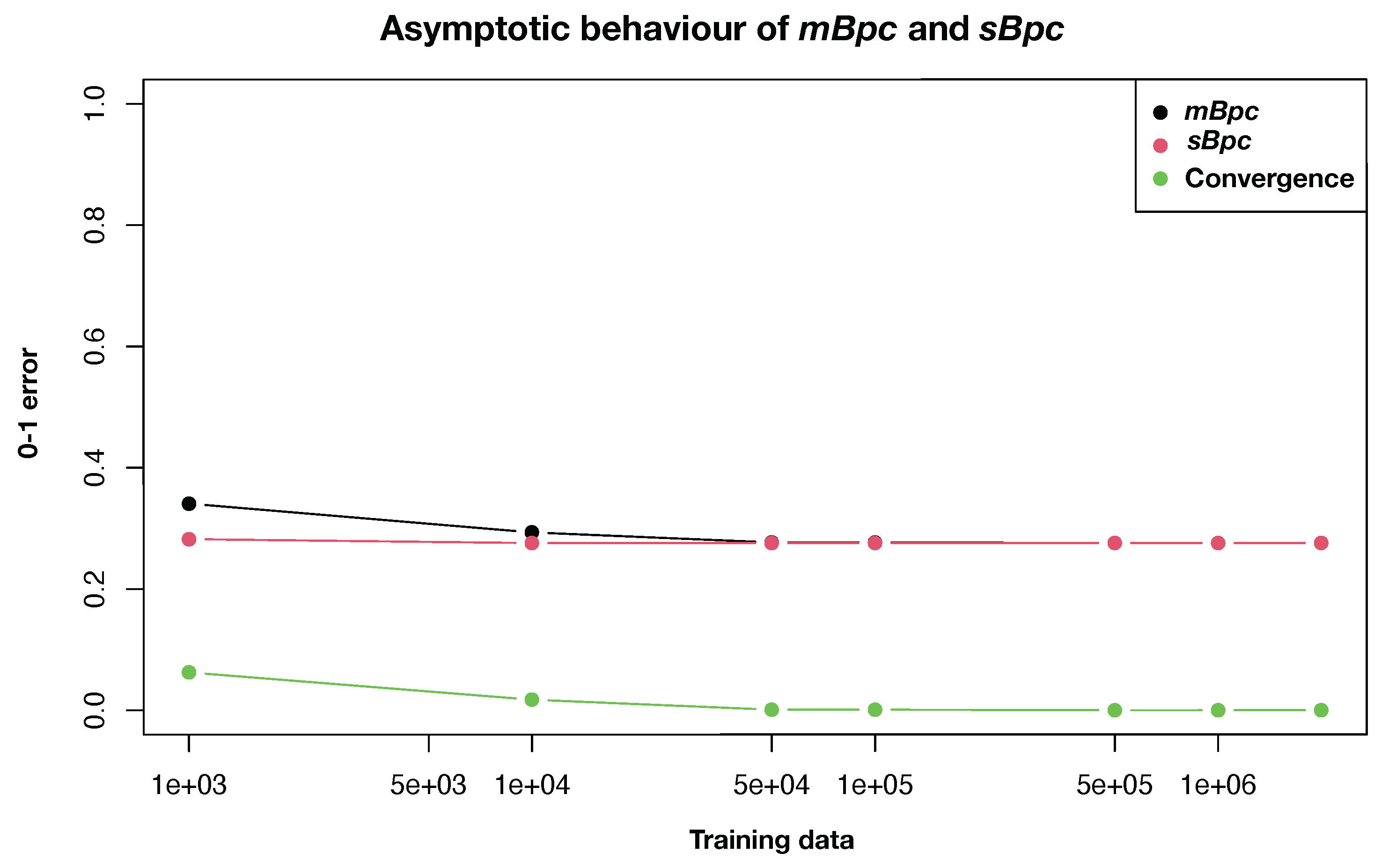
4. Numerical Illustrations Underlying Convergence

To study the classification performance and convergence of the two different classifiers, we simulated both training and test datasets from the PD distribution with a generative urn model described in [10] called the De Morgan process. We varied the amount of training and test data, the values of the distribution parameter ψ , as well as the amount of classes k. A pool of 4 million data points was created for each ψ . A small sample of size 1000 was used to train the model first. This sample was augmented with more data from the same pool for each ψ up to 2 million (without replacement) to form our two small and big training data sizes. A test dataset created with the same parameters was kept constant for classification with all training data samples as reflected in Table 1 and Figure 1.
The above results next to our experiments show that the simultaneous classifier performs better than the marginal classifier especially as the number of the classes is higher and training data is small. As the amount of training data increases, the predictions of the classifiers converge, as the extra information in the test data used by the simultaneous classifier becomes negligible. This behaviour is illustrated in Figure 1. Additionally, the first row of the Table 1 shows that the classifier fails on the binary classification task with datasets created with ψ of 1 and 2. This is because the classes created with ψ of such similar magnitude will be distributed very similarly, tailored both from similarity of these values and their closeness to zero. Thus the classification results are no better than random guessing (accuracy of 0.491). The data is in fact so homogeneous in this case, that the labelings of the two different classifiers already converge with test data of size 1000. On the other hand, the biggest difference underlies the 4th row where, despite a clear distinction between the competing classes ψ , the sBpc is distinctively performing better than mBpc but both predictions are even worse than random guessing. This is due to the small training samples and, as marked, the improvement is considerable for each classifier and also their difference is decreasing. Compared with the three-class groups of the second and third row of the Table 1, we conclude that the number of classes is playing a more pivotal role in accuracy of the classifiers than the distinction between the underlying dispersal parameters. However, this dominating factor is in service to the number of training data as well such that increasing amount of training data could overrule this differentiating cause.
Altogether, the above results support the hypothesis that the marginal and simultaneous classifiers converge in their labelings with enough training data. This justifies the use of the marginal classifier in place of the more accurate simultaneous one with large data. Still, the simultaneous classifier is more accurate with smaller training data, as it benefits from the information in the test data.

5. Discussion

Previously unseen or unanticipated feature values are challenging scenarios in standard Bayesian inductive inference. Under general exchangeability as formalized by de Finetti, upon such an observation, the entire alphabet of anticipated feature values must be retrospectively changed. Due to consideration of the specificity of the type of data being generated under PE, the classifiers introduced here, however, are based on a fully probabilistic framework and, as such, are equipped with a specific formulation that allow the updating of their predictions autonomously. This choice of classifiers are shown to have multiple advantages in population structure studies where there is a need for accommodating the appearance of the unseen species [21]. The classification of previously unseen feature values here is handled through the use of a parameter learned from the training data, instead of, for example, using an uninformative Dirichlet-prior [6]. The superiority in classification accuracy of labeling the test data simultaneously instead of one by one was also shown under partition exchangeability. The assumption that test data is i . i . d . is obviously an unrealistic one. The two classifiers considered here only converge in prediction as the amount of training data approaches infinity. This is a special case of the coincidence of the exchangeablity laws in the limiting forms for the mixture of the infinitely divisible distributions under specific conditions [22]. From the computational point of view, however, the simultaneous classifier exhibits the exponentially increasing cost as the amount of test data increases, making it unfeasible to use for large-scale prediction. Additionally, the algorithm presented here is only capable of arriving at local optima, leaving still the chances of being sub-optimal in multimodal scenarios. Further research could be directed at the Gibbs sampler-assisted algorithms presented in [5] to more thoroughly scan the optimization space, although the convergence of such algorithms with large test datasets is also uncertain. An implementation for the supervised classifiers considered could also be extended for the two parameter distribution Poisson–Dirichlet ( α , ψ ) [23] (Appendix C).

6. Conclusions

We provided an estimation and hypothesis testing scheme for the dispersal parameter of the PD distribution tied with the sequences under PE. These derivations next to the algorithms for the computational calculation of the simultaneous and marginal Bayesian predictive classifiers and their implementations as a software package PEkit (https://cran.r-project.org/web/packages/PEkit/index.html, accessed on 23 December 2021 ) in R, would facilitate the smoother application of these classifiers and provides a conductive avenue toward PEs more effective disposition and prevalence in the community. In short, we provided the computational evidence that the marginal and simultaneous predictive classifiers under partition exchangeability converge in their classification assignment with presence of umpteen amount of training data. This asymptotic convergence of the classifiers, justifies the interchangeable use of them and hence, legitimizing forgoing of the sPpc’s negligible superiority in accuracy, for the mPpc’s huge computational advantage. Of course, under reasonably small amount of training data, this would be more of a preferential interplay, but altogether, these Bayesian classifiers are robust probabilistic judgmental apparatus for supervised classification tasks in the inductive inference domain. Next to these results, we underlie the presented derivations and exclusive tool for PE sequences. Namely, the hypothesis testing paradigm, random generation of the PD distribution, and its numerical MLE formulation, would be of a great use for the experiments underlying species sampling sequences.

Author Contributions

Conceptualization, A.A.; methodology, A.A. and V.K.; software, A.A. and V.K.; validation, A.A.; formal analysis, A.A. and V.K.; investigation, A.A. and V.K.; resources, J.T.; data curation, A.A. and V.K.; writing—original draft preparation, A.A. and V.K.; writing—review and editing, A.A. and J.T.; visualization, A.A. and V.K.; supervision, A.A.; project administration, A.A. and J.T.; funding acquisition, J.T. All authors have read and agreed to the published version of the manuscript.

Funding

This research was funded by Academy of Finland grant No. 320131.

Institutional Review Board Statement

Not applicable.

Informed Consent Statement

Not applicable.

Data Availability Statement

The package for Bayesian predictive supervised classifications, parameter estimation and hypothesis testing of the Ewens Sampling Formula generative model as well as the synthetic data used in this article is deposited on CRAN as PEkit package (https://cran.r-project.org/web/packages/PEkit/index.html, accessed on 23 December 2021 and https://github.com/AmiryousefiLab/PEkit, accessed on 23 December 2021).

Conflicts of Interest

The authors declare no conflict of interest.

Abbreviations

The following abbreviations are used in this manuscript:
PEPartition Exchangeability
mBpcmarginal Bayesian predictive classifiers
sBpcsimultaneous Bayesian predictive classifiers
LRTLikelihood Ratio Test
MLEMaximum Likelihood Estimate
PDPoisson–Dirichlet
i.i.d.Independent and Identically Distributed

Appendix A. Maximum Likelihood Estimate

Here we provide the technical details for deriving the MLE in Equation (3) as well as the components U and I in the Lagrange Multiplier test described in Equations (5) and (6). The task is to find the first derivative of the logarithm of the Ewens sampling formula and its root in Equation (2), as well as the second derivative needed for the Fisher information.
L ( ψ ) = l o g ( n ! ) + i = 1 n { l o g ( ψ + i 1 ) + ρ i l o g ψ ρ i l o g ρ i l o g ( ρ i ! ) } = > l ( ψ ) = i = 1 n { l o g ( ψ + i 1 ) + ρ i l o g ψ }
l ( ψ ) = i = 1 n 1 ψ + i 1 + ρ i ψ = U ( ψ )
The MLE is found by finding the root of the equation:
i = 1 n 1 ψ ^ + i 1 + ρ i ψ ^ = 0 j = 1 n ψ ^ ψ ^ + j + 1 = t = 1 n ρ t

Appendix B. Lagrange Multiplier Test

According to Ewens in [15], the left side of the above equation equals the expected number of unique values observed with this ψ and this sample size n, while the right side is the observed number of unique values:
E [ t = 1 n ρ t | ψ , n ] = i = 1 n ψ ^ ψ ^ + i 1
This is needed for the Fisher information I, along with the second derivative of l ( ψ ) :
l ( ψ ) = i = 1 n 1 ( ψ + i 1 ) 2 ρ i ψ 2 = i = 1 n 1 ( ψ + i 1 ) 2 k i = 1 n ψ 2 ,
where k denotes the observed amount of unique values in the sample. The Fisher information then becomes:
I ( ψ ) = E [ l ( k ; ψ ) | ψ ] = E [ k | ψ ] i = 1 n ψ 2 i = 1 n 1 ( ψ + i 1 ) 2 = i = 1 n 1 ψ ( ψ + i 1 ) 1 ( ψ + i 1 ) 2 ,
where the expectation of k is as described from above.

Appendix C. A Note on Two-Parameter PD

A two-parameter formulation of the distribution presented in [23]. The added parameter in PD ( α , ψ ) is called the discount parameter. The role of the parameters is discussed in length in [16]. In short, the α is defined to fall in the interval [ 1 , 1 ] . When it is positive, it increases the probability of observing new species in the future proportional to the amount of already discovered species, while decreasing the probability of seeing the newly observed species again. When α is negative, the opposite is true and the number of new species to be discovered is bounded. The single parameter P D ( ψ ) is the special case of the two parameter distribution with α set to 0, P D ( 0 , ψ ) . The two parameter distribution is not considered further here, as the estimation of the parameters becomes a daunting task compared to the simple one parameter formalization.

References

  1. Solomonoff, R. A formal theory of inductive inference. Inf. Ctrl. 1964, 7, 1–22. [Google Scholar]
  2. Falco, I.D.; Cioppa, A.D.; Maisto, D.; Tarantino, E. A genetic programming approach to Solomonoff’s probabilistic induction. In European Conference on Genetic Programming; Springer: Berlin/Heidelberg, Germany, 2006; pp. 24–35. [Google Scholar]
  3. Hand, D.J.; Yu, K. Idiot’s Bayes: Not so stupid after all? Int. Stat. Rev. 2001, 69, 385. [Google Scholar]
  4. Bryant, P.; Williamson, J.A. Asymptotic behaviour of classification maximum likelihood estimates. Biometrika 1978, 65, 273–281. [Google Scholar] [CrossRef]
  5. Corer, J.; Cui, Y.; Koski, T.; Siren, J. Have I seen you before? Principles of Bayesian predictive classification revisited. Springer Stat. Comput. 2011, 23, 59–73. [Google Scholar]
  6. Quintana, F.A. A predictive view of Bayesian clustering. J. Stat. Plan. Inference 2006, 136, 2407–2429. [Google Scholar] [CrossRef]
  7. Bassetti, F.; Ladelli, L. Mixture of Species Sampling Models. Mathematics 2021, 9, 3127. [Google Scholar] [CrossRef]
  8. Barlow, R.E. Introduction to de Finetti (1937) foresight: Its logical laws, its subjective sources. In Breakthroughs in Statistics; Springer: New York, NY, USA, 1992; pp. 127–133. [Google Scholar]
  9. Kingman, J.F.C. Random partitions in population genetics. Proc. R. Soc. A Math Phys. Eng. Sci. 1978, 361, 1–20. [Google Scholar]
  10. Zabell, S.L. Predicting the unpredictable. Harv. Bus. Rev. 1992, 90, 205–232. [Google Scholar] [CrossRef]
  11. Hansen, B.; Pitman, J. Prediction rules for exchangeable sequences related to species sampling. Stat. Probab. Lett. 2000, 46, 251–256. [Google Scholar] [CrossRef]
  12. Bassetti, F.; Ladelli, L. Asymptotic number of clusters for species sampling sequences with non-diffuse base measure. Stat. Probab.-Lett. 2020, 162, 108749. [Google Scholar] [CrossRef]
  13. Amiryousefi, A. Asymptotic Supervised Predictive Classifiers under Partition Exchangeability. arXiv 2021, arXiv:2101.10950. [Google Scholar]
  14. Kingman, J.F.C. The population structure associated with the Ewens sampling formula. Theor. Popul. Biol. 1977, 11, 274–283. [Google Scholar] [CrossRef]
  15. Ewens, W. The Sampling Theory of Selectively Neutral Alleles. Theor. Popul. Biol. 1972, 3, 87–112. [Google Scholar] [CrossRef]
  16. Crane, H. The Ubiquitous Ewens Sampling Formula. Stat. Sci. 2016, 31, 1–19. [Google Scholar] [CrossRef]
  17. Radhakrishna Rao, C. Large sample tests of statistical hypotheses concerning several parameters with applications to problems of estimation. Math. Proc. Camb. Philos. Soc. 1948, 44, 50–57. [Google Scholar] [CrossRef]
  18. Neyman, J.; Pearson, E.S. On the problem of the most efficient tests of statistical hypotheses. Philos. Trans. R. Soc. Lond. Ser. A Contain. Pap. Math. Phys. Character 1933, 231, 289–337. [Google Scholar] [CrossRef] [Green Version]
  19. Hoppe, F.M. Polya-like urns and the Ewens sampling formula. J. Math. Biol. 1984, 20, 91–94. [Google Scholar] [CrossRef] [Green Version]
  20. Karlin, S.; McGregor, J. Addendum to a paper of Ewens. Theor. Popul. Biol. 1972, 3, 113–116. [Google Scholar] [CrossRef]
  21. Corer, J.; Gyllenberg, M.; Koski, T. Random partition models and exchangeability for Bayesian identification of population structure. Bull. Math. Biol. 2007, 69, 797–815. [Google Scholar]
  22. Fortini, S.; Ladelli, L.; Regazzini, E. A Central Limit Problem for Partially Exchangeable Random Variables. Theory Probab. Its Appl. 1997, 41, 224–246. [Google Scholar] [CrossRef] [Green Version]
  23. Pitman, J.; Yor, M. The two-parameter Poisson-Dirichlet distribution derived from a stable subordinator. Ann. Probab. 1997, 25, 855–900. [Google Scholar] [CrossRef]
Figure 1. The classification error of the marginal and simultaneous classifiers with datasets from PD distribution with ψ ( 1 , 10 , 50 ) , as well as the convergence of their labellings. Rows 2 and 3 in Table 1 are included in the figure.
Mathematics 10 00828 g001
Table 1. The item-wise 0–1 classification error for the marginal and simultaneous classifiers, as well as the 0–1 absolute difference between the predicted labels between the two classifiers ( δ ).
Training (m)Test (n)No. Clusters (k)Dispersion ( ψ ) p ^ m B p c p ^ s B p c | δ |
2 × 10 6 2 × 10 3 21, 20.4910.4910
10 3 2 × 10 3 31, 10, 500.34080.28230.0626
10 5 2 × 10 3 31, 10, 500.27680.27580.0010
10 3 2 × 10 3 51, 100, 10 3 , 5 × 10 3 , 10 4 0.75350.58650.167
2 × 10 6 2 × 10 3 51, 100, 10 3 , 5 × 10 3 , 10 4 0.4340.3640.115
Publisher’s Note: MDPI stays neutral with regard to jurisdictional claims in published maps and institutional affiliations.

