Infinite–Dimensional Bifurcations in Spatially Distributed Delay Logistic Equation

Abstract

This paper investigates the questions about the local dynamics in the neighborhood of the equilibrium state for the spatially distributed delay logistic equation with diffusion. The critical cases in the stability problem are singled out. The equations for their invariant manifolds that determine the structure of the solutions in the equilibrium state neighborhood are constructed. The dominant bulk of this paper is devoted to the consideration of the most interesting and important cases of either the translation (advection) coefficient is large enough or the diffusion coefficient is small enough. Both of this cases convert the original problem to a singularly perturbed one. It is shown that under these conditions the critical cases are infinite–dimensional in the problems of the equilibrium state stability for the singularly perturbed problems. This means that infinitely many roots of the characteristic equations of the corresponding linearized boundary value problems tend to the imaginary axis as the small parameter tends to zero. Thus, we are talking about infinite–dimensional bifurcations. Standard approaches to the study of the local dynamics based on the application of the invariant integral manifolds methods and normal forms methods are not applicable. Therefore, special methods of infinite–dimensional normalization have been developed which allow one to construct special nonlinear boundary value problems called quasinormal forms. Their nonlocal dynamics determine the behavior of the initial boundary value problem solutions in the neighborhood of the equilibrium state. The bifurcation features arising in the case of different boundary conditions are illustrated.

1. Introduction

We consider the spatially distributed delay logistic equation

$$\frac{\partial u}{\partial t}=d\frac{{\partial }^{2}u}{\partial x^2}+b\frac{\partial u}{\partial x}+r[1-u(t-T,x)]u$$

(1)

with the periodic boundary conditions

$$u(t,x+2\pi )\equiv u(t,x).$$

(2)

The coefficient $d>0$ is called the diffusion coefficient or the mobility coefficient when it comes to a biological population. The coefficient $r>0$ is called the Malthusian coefficient and $T>0$ is the delay time. The presence of the translation operator $b\partial u/\partial x$ in the boundary value problem (1), (2) differs from the logistic equation with diffusion. The coefficient b in this operator can be considered positive. The function $u(t,x)$ makes sense of the population density and therefore $u(t,x)\ge 0$. The translation operator is irrelevant for the boundary value problem without delay

$$\frac{\partial }{\partial t}u=d\frac{{\partial }^{2}u}{\partial x^2}+b\frac{\partial u}{\partial x}+r[1-u]u,u(t,x+2\pi )\equiv u(t,x).$$

(3)

It ‘disappears’ after the spatial variable replacement $x\to x+bt$.

An equation of the (1) type arises in many applied problems of mathematical ecology and mathematical biology (see, for example, [1,2,3,4,5,6,7]). The most complete research results are presented in [8,9,10].

In this paper, we study the local dynamics of the boundary value problem (1), (2) in a neighborhood of a positive equilibrium state, that is, the behavior of the (1), (2) solutions with initial conditions from some sufficiently small neighborhood of the equilibrium state $u_0\equiv 1$. We fix the space ${\mathbf{C}}_{[-T,0]}\times {\mathbf{W}}_{2[0,2\pi ]}^2$ as the space of initial conditions. We pay special attention to the study of cases when either the translation coefficient b is sufficiently large or the diffusion coefficient is sufficiently small. It is in these cases that the boundary value problem (1), (2) becomes singularly perturbed, which can lead to the appearance of new interesting dynamic effects.

We recall the well-known (see, for example, [11,12]) results for the delay logistic equation

$$\dot{u}=r[1-u(t-T)]u.$$

(4)

Under the condition $rT\le \pi /2$, the equilibrium state $u_0\equiv 1$ is asymptotically stable, and it is unstable when $rT>\pi /2$ and there is a stable cycle in (4). The asymptotic behavior of this cycle under the condition $0<rT-\pi /2\ll 1$ is given in [13]. Questions about the global stability of Equation (4) are studied in [11,12,14].

Under the condition $rT\gg 1$, the asymptotic stability of the cycle is described in [15]. We recall a well-known result of the Andronov–Hopf bifurcation in (4) under the conditions $rT\approx \frac{\pi }{2}$. We fix the values $r_0$ and $T_0$ in (4) so that $r_0{T}_0=\frac{\pi }{2}$. Let

$$r=r_0+\epsilon r_1,T=T_0+\epsilon T_1$$

(5)

where $\epsilon$ is a small positive parameter:

$$0<\epsilon \ll 1.$$

Then in some sufficiently small and $\epsilon$ independent neighborhood of Equation (4) solution $u_0$ there exists [16,17,18] a stable local invariant integral two-dimensional manifold $M\left(\epsilon \right)$ on which Equation (4) can be written in the form of a scalar complex ordinary differential equation

$$\frac{d\xi }{d\tau }=\alpha \xi +\sigma \xi {\left|\xi \right|}^2$$

(6)

to within $O\left(\epsilon \right)$. Here, $\tau =\epsilon t$ is a ‘slow’ time and

$$\begin{array}{ccc}\hfill \alpha & =& {\left(1+\frac{{\pi }^2}{4}\right)}^{-1}\left[\left(\frac{\pi }{2}+i\right)r_1+{\lambda }_0^2{T}_1\left(1-i\frac{\pi }{2}\right)\right],\hfill \\ \hfill \sigma & =& -{\lambda }_0\left[3\pi -2+i(\pi +6)\right]{\left(10(1+\frac{4}{{\pi }^2})\right)}^{-1},\Re \sigma <0.\hfill \end{array}$$

Equation (6) is called the normal form for (1), (2) in the neighborhood of $u_0$. The solutions (6) and (4) are related by the asymptotic equality

$$u=1+{\epsilon }^{1/2}\left(\xi \left(\tau \right)exp\left(i\pi {\left(2T_0\right)}^{-1}t\right)+\overline{\xi }\left(\tau \right)exp\left(-i\pi {\left(2T_0\right)}^{-1}t\right)\right)+O\left(\epsilon \right).$$

(7)

Accordingly, the cycle in (6) corresponds to the stable cycle in (4) (as $\Re \alpha >0$).

Under the conditions (5) and for $b=0$, the same manifold $M\left(\epsilon \right)$ is a stable invariant manifold for the delay logistic equation with diffusion

$$\frac{\partial u}{\partial t}=d\frac{{\partial }^{2}u}{\partial x^2}+r[1-u(t-T,x)]u,u(t,x+2\pi )\equiv u(t,x).$$

(8)

Therefore, the equilibrium state of $u_0$ is stable as $rT\le \frac{\pi }{2}$ and is unstable as $rT>\frac{\pi }{2}$ for this equation, and the same cycle as in Equation (4) exists. The cycle bifurcation for (4) and (8) is of the Andronov–Hopf type [10,19]. There is only one pair of pure imaginary roots, whereas other roots of the characteristic equations for the linearized on $u_0$ equations have negative real parts as $\epsilon =0$.

We get back to the boundary value problem (1), (2) consideration. Its local dynamics in the equilibrium state of $u_0$ neighborhood depend largely on the behavior of solutions of the linearized on $u_0$ boundary value problem

$$\frac{\partial v}{\partial t}=d\frac{{\partial }^{2}v}{\partial x^2}+b\frac{\partial v}{\partial x}-rv(t-T,x),v(t,x+2\pi )\equiv v(t,x).$$

(9)

In turn, the behavior of Equation (9) solutions is related to the location of the roots of its characteristic quasi-polynomial, which consists of the set of the equations

$$\lambda =-d{k}^2+ibk-rexp(-\lambda T),k=0,\pm 1,\pm 2,\dots .$$

(10)

In the case when the roots of (10) have negative real parts, all the solutions of (9) tend to zero as $t\to \infty$ and the equilibrium state of $u_0$ is asymptotically stable in (1), (2). However, if a root with a positive real part exists in (10), then (9) has a solution that grows exponentially as $t\to \infty$ and the solution of $u_0$ in (1), (2) is unstable.The critical case in the problem of $u_0$ stability takes place under the condition that (10) has no roots with positive real part, but a root with zero real part exists.

In this paper, we focus our attention on the determination of the parameters for which critical cases take place and on the study of the (1), (2) solutions in near-critical situations.

Below we show that the bifurcation phenomena are much more complicated and diverse for the boundary value problem (1), (2) than those that take place for the boundary value problem (8). In the case of singular perturbations when $b\gg 1$ or $d\ll 1$ some interesting situations may arise when infinitely many roots of the characteristic Equation (10) tend to the imaginary axis as the small parameter tends to zero. Thus, the critical case of infinite dimension is realized in the problem of the solutions stability. Note that singular perturbations in a nonlocal setting were studied, for example, in [20,21,22].

Special nonlinear equations that do not contain small parameters are constructed as the main results. Their nonlocal dynamics determine the behavior of the boundary value problem (1), (2) solutions in the neighborhood of the equilibrium state of $u_0$. These equations are classical normal forms on invariant manifolds in finite-dimensional critical cases. There are no invariant manifolds in infinite-dimensional critical cases, but the formal method of normal forms allows us to construct special boundary value problems of the parabolic type, the so-called quasinormal forms, which play the role of normal forms. Asymptotic formulas that couple the solutions of the initial problem and the solutions of the quasinormal forms are given.

In the next section, the critical cases are defined on the basis of the characteristic Equation (10) roots analysis, and the bifurcations when the parameter b is changed are studied. Moreover, main attention is paid to the singularly perturbed case when $b\gg 1$. The most interesting situations that arise at asymptotically small values of the diffusion coefficient d are considered in Section 3. The infinite-dimensional bifurcations for the Dirichlet boundary conditions with sufficiently large values of the delay coefficient are considered in Section 4. Finally, the conclusions are formulated in Section 5.

2. Determined by Translation Coefficient b Bifurcations

In this section, we first focus on the analysis of the characteristic Equation (10) roots, and then we consider the bifurcation problem of constructiong a normal form. In the final part, we investigate the dynamics of the boundary value problem (1), (2) for large values of b.

2.1. Linear Analysis

We assume $\lambda =i\omega$ where $\omega >0$ to construct the boundaries of the stability domain in the space of parameters of Equation (10) for some $k=k_0$. We obtain from (10) that

$$i\omega =-d{k}_0^2+ib{k}_0-rexp(-i\omega T).$$

(11)

This equation is equivalent to the system of two equations

$$\begin{array}{ccc}\hfill rcos\omega T& =& -d{k}_0^2,\hfill \end{array}$$

(12)

$$\begin{array}{ccc}\hfill rsin\omega T& =& \omega -b{k}_0.\hfill \end{array}$$

(13)

2.1.1. Case of $k_0=0$

From (10) we obtain the equation

$$\lambda =-rexp(-i\lambda T)$$

(14)

which is a well-known characteristic equation for the classical delay logistic equation. Therefore, we conclude that there is a root with a positive real part in (14) and hence in (10) under the condition $rT>\frac{\pi }{2}$.

Below we assume that the inequality

$$rT\le \frac{\pi }{2}$$

(15)

holds.

There is a pair of the complex conjugate roots ${\lambda }_{1,2}=\pm i\pi {\left(2T\right)}^{-1}$ for $rT=\frac{\pi }{2}$ and the other roots of (14) have negative real parts.

2.1.2. Case of $k_0=1$

We state one simple proposition first.

Lemma 1.

Let the inequalities

$$rT<\frac{\pi }{2},0<r<d$$

(16)

hold. Then the roots of Equation (10) have negative real parts.

Indeed, it follows from (16) that Equations (12) and (13) are unsolvable.

We consider the case where $k=1$ and $r=d$. It then follows from (12) that the equality $\omega T=\pi (2n+1)$ holds for some integer n, and from (13) we obtain that $\pi (2n+1)T^{-1}=b$. Below, let $T_k(r,b)(k=0,1,2,\dots )$ stand for such a value of the parameter T that for $0<T<T_k(r,b)$ the roots of (10) have negative real parts for the given k, and there is a root on the imaginary axis as $T=T_k(r,b)$. Thus, $T_0(r,b)=T_0\left(r\right)=\pi {\left(2r\right)}^{-1}$, and under the condition $r=d$ the equality $T_1(d,b)=\pi b^{-1}$ holds.

Further, we consider the case where

$$d<r\le 4d.$$

Under this condition and for all values of the parameters b and T, the roots of all of Equation (10) have negative real parts as $\left|k\right|>1$. From (12), (13) we conclude that

$$T_1(r,b)={\phi }_1{\left[b+\sqrt{r^2-d^2}\right]}^{-1},cos{\phi }_1=-d{r}^{-1},{\phi }_1\in \left(\frac{\pi }{2},\pi \right).$$

We note that $T_1(r,0)>T_0\left(r\right)$ and $\underset{b\to \infty }{lim}{T}_1(r,b)=0$, therefore there is such $b=b_0$ that $T_1(r,b_0)=T_0\left(r\right)$. In this case, each element of Equation (10) has pure imaginary roots as $k=0$ and $k=\pm 1$. For example, the equality $T_1(d,b)=\pi b^{-1}=T_0\left(d\right)=\pi {\left(2d\right)}^{-1}$ holds as $r=d$. Thus, $b_0=2d$, and $T_1(4d,b)=\pi {\left(2b\right)}^{-1}=\pi {\left(8d\right)}^{-1}$ as $r=4d$, i.e., $b_0=4d$.

2.1.3. Case of $k_0>1$

Let $k>1$ and the inequality

$$r>d{k}^2$$

holds. Acting in accordance with the previous scheme, we obtain that

$$T_1(r,b)={\phi }_k{\left(b_k+{\left(r^2-d{k}^2\right)}^{1/2}\right)}^{-1},cos{\phi }_k=-d{k}^2{r}^{-1},\frac{\pi }{2}<{\phi }_k<\pi .$$

Let $k_0$ stand for the largest integer $k>0$ for which the inequality $d{k}_0^2\le r$ holds.

We assume that

$$T_{min}(r,b)=min\left(T_0\left(r\right),T_1(r,b),\dots ,T_{k_0}(r,b)\right).$$

Lemma 2.

Under the condition $0<T<T_{min}(r,b)$ the roots of the characteristic Equation (10) have negative real parts, and Equation (10) has no roots with positive real part but the root on the imaginary axis as $T=T_{min}(r,b)$.

It is important to note that the parameter T increment from $T_{min}(r,b)$ to $T_0\left(r\right)$ in the boundary value problem (9) can lead to several alternations of stability and instability of solutions.

The following statement is more interesting.

Lemma 3.

Let the solutions of (9) be unstable for some value of the parameter b. Then stability and instability of the (9) solutions alternate infinitely as $b\to \infty$.

Since ${\left(d{k}_0^2\right)}^2+{\left(\omega -b{k}_0\right)}^2=r_0^2$, we obtain two values

$${\omega }_{1,2}=b{k}_0\pm \sqrt{r_0^2}-{\left(d{k}_0^2\right)}^2$$

for $\omega$. We note that ${\omega }_1>\left|{\omega }_2\right|$. Let $T_1^{+},T_2^{+},\dots$ stand for the consecutive positive roots (in relation to T) of the equation $d{k}_0^2=-r_{0}cos{\omega }_{1}T$. In addition, let $T_1^{-},T_2^{-},\dots$ stand for the consecutive positive roots of the equation $d{k}_0^2=-r_{0}cos{\omega }_{2}T$. We note that $T_{2n+1}^{+}=T_1^{+}+2\pi n{\omega }_1^{-1}$, $T_{2n+2}^{-}=T_2^{-}+2\pi {\omega }_2^{-1}$ and $T_1^{+}<T_2^{-}$. It is evident that the values $T_{2n-1}^{+}$ and $T_{2n}^{-}(n=1,2,\dots )$ only are the roots of the system of Equation (10) for $\omega ={\omega }_1$ and $\omega ={\omega }_2$, respectively. Let $\lambda \left(T\right)$ stand for such a root of (10) that turns into $i{\omega }_1$ and $i{\omega }_2$ for $T=T_{2n-1}^{+}$ or $T=T_{2n}^{-}$, respectively. Then, for $k=k_0$ we obtain from (10) that

$$\frac{d\lambda \left(T\right)}{dT}{|}_{\genfrac{}{}{0.0pt}{}{T=T_{2n-1}^{+}}{T=T_{2n}^{-}}}={\left[{(1-r_{0}Tcos\omega T)}^2+r_0^2{T}^2{sin}^2\omega T\right]}^{-1}\omega (\omega -b{k}_0)$$

where $\omega ={\omega }_1$ as $T=T_{2n+1}^{+}$, and $\omega ={\omega }_2$ as $T=T_{2n}^{-}$. From (10), it now follows that

$$\frac{d\lambda \left(T\right)}{dT}{|}_{T=T_{2n-1}^{+}}>0,\mathrm{and}\mathrm{for}{\omega }_2<0\mathrm{we}\mathrm{obtain}\frac{d\lambda \left(T\right)}{dT}{|}_{T=T_{2n}^{-}}>0.$$

If ${\omega }_2>0$ then $\frac{d\lambda \left(T\right)}{dT}{|}_{T=T_{2n}^{-}}<0$. From here we obtain the following statements:

1.

If $0\le T<T_1^{+}$ then the roots of (10) have negative real parts as $k=k_0$;

2.

If ${\omega }_2<0$ and $T>T_1^{+}$ then Equation (10) has a root with positive real part as $k=k_0$;

3.

If ${\omega }_2>0$ and $T_1^{+}<T<T_2^{-}$ then Equation (10) has a root with positive real part as $k=k_0$;

4.

If ${\omega }_2>0$ and $T_3^{+}<T_2^{-}$ then Equation (10) has a root with positive real part for all $T>T_1^{+}$ as $k=k_0$;

5.

If ${\omega }_2>0$ and $T_2^{-}<T<T_3^{+}$ then the roots of (10) have negative real parts as $k=k_0$. More generally, under the conditions $T_{2n}^{-}<T<T_{2n+1}^{+}$ the roots of (10) have negative real parts as $k=k_0$.

The resulting domain of instability (in the space of parameters) of the characteristic Equation (10) is an union of the instability domains of each of the equations that make up (10). Thus, a situation is possible when this domain consists of one or several (because their number is finite) intervals.

2.2. Andronov–Hopf Bifurcation

Let for some $T=T_0$ and $k=k_0$ (the case of $k=0$ is studied in [19]) the characteristic Equation (10) has one pure imaginary root $\lambda =i\omega$, whereas all the other roots have negative real parts (as $k\ge 0$). We assume $\omega ={\omega }_{1,2}$ and let the equalities (5) hold. We consider the behavior of the (8) solutions with initial conditions from some rather small ($\epsilon$–independent) neighborhood of the equilibrium state $N\equiv 1$. According to the general theory (see, for example, [16,17,18]) in this neighborhood there is a local invariant two-dimensional stable integral manifold on which (8) can be presented as a normal form

$$\frac{d\xi }{d\tau }={\alpha }_1\xi +{\beta }_1{\left|\xi \right|}^2{\xi }_n(\tau =\epsilon t)$$

(17)

to within $O\left(\epsilon \right)$. We put $z=\omega t+k_{0}x$ to obtain explicit expressions for the coefficients ${\alpha }_1$ and ${\beta }_1$, and introduce the formal series

$$\begin{array}{c}N=1+{\epsilon }^{\frac{1}{2}}\left[\xi \left(\tau \right)exp\left(iz\right)+\overline{\xi }\left(\tau \right)exp(-iz)\right]+\hfill \\ +\epsilon \left[u_{20}\left(\tau \right)\left|{\xi }^2\left(\tau \right)\right|+u_{21}\left(\tau \right){\xi }^2\left(\tau \right)exp\left(2iz\right)+{\overline{u}}_{21}\left(\tau \right){\xi }^{-2}\left(\tau \right)exp(-2iz)\right]+\\ \hfill +{\epsilon }^{\frac{3}{2}}\left[u_{31}\left(\tau \right)exp\left(iz\right)+{\overline{u}}_{31}\left(\tau \right)exp(-iz)+u_{33}\left(\tau \right)exp\left(3iz\right)+{\overline{u}}_{33}\left(\tau \right)exp(-3iz)\right]+\dots .\end{array}$$

(18)

Substituting (18) into (1) and collecting the coefficients at the equal powers of $\epsilon$ we obtain in the second step that

$$\begin{array}{ccc}\hfill u_{20}& =& 2r_0^{-1}cos\omega T_0,\hfill \\ \hfill u_{21}& =& -r_0{\left(2i\omega +4d{k}_0^2-2ib{k}_0+r_{0}exp(-2T_0\omega )\right)}^{-1}exp(-i\omega T_0).\hfill \end{array}$$

From the solvability condition of the resulting equation with respect to $u_{31}$ (and ${\overline{u}}_{31}$), we arrive at a relation for the unknown value $\xi \left(\tau \right)$, which has the form of (17) in which

$$\begin{array}{ccc}\hfill {\alpha }_1& =& i{r}_0\omega T_1{(1-r_0{T}_{0}exp(-i\omega T_0))}^{-1},\hfill \\ \hfill {\beta }_1& =& -r_0{(1-r_0{T}_{0}exp(-i\omega T_0))}^{-1}\times \hfill \\ & \times & \left[u_{20}(1+exp(-i\omega T_0))+u_{21}(exp\left(i\omega T_0\right)+exp(-2i\omega T_0))\right].\hfill \end{array}$$

We note that the sign of the value $\Re \left({\alpha }_1\right)$ coincides with the sign of the expression $\omega (\omega -b)$.

The stability of the equialibrium state of $u_0$ of the boundary value problem (1), (2) for small values of $\epsilon$ is obviously determined by the sign of $\Re \left({\alpha }_1\right)$, and the existence and stability of the cycle in (1), (2) are related to the existence of the cycle in (17), i.e., to the signs of the values $\Re \left({\alpha }_1\right)$ and $\Re \left({\beta }_1\right)$.

2.3. Local Dynamics in the Case of Large Translation Coefficient

Here we assume that the parameter b is large enough:

$$b={\epsilon }^{-1},0<\epsilon \le 1.$$

(19)

It then follows from equality (13) that the quantity $\omega$ is of the order of ${\epsilon }^{-1}$, and the corresponding values of T at which the stability of the equilibrium state can change are of the order of $\epsilon$. In this regard, it is natural to set $T=\epsilon T_1$ and change the time $t=\epsilon t_1$ in (1). Below, it is convenient to replace u with $u-1$ in (1). Then the corresponding boundary value problem with respect to $u_1=u-1$ after multiplying by $\epsilon$ of the left and right parts can be written in the form

$$\frac{\partial u}{\partial t_1}=\epsilon \left[d\frac{{\partial }^{2}u}{\partial x^2}-r_{0}u(t_1-T_1,x)(1+u)\right]+\frac{\partial u}{\partial x},$$

(20)

$$u(t_1,x+2\pi )\equiv u(t,x).$$

(21)

Formally assuming $\epsilon =0$, we arrive at a linear equation whose entire stability spectrum is pure imaginary. Thus, the critical case of infinite dimension is realized in the problem of the equilibrium state of (20), (21) stability. An algorithm for studying the dynamic properties of solutions in such situations is developed in [23,24]. We apply the corresponding constructions for (20), (21). We introduce the formal expression

$$\begin{array}{c}\hfill u=\sum _{n=-\infty }^{\infty }{\xi }_n\left(\tau \right)expik(t_1+x)+\epsilon v(\tau ,y)+\dots =\xi (\tau ,y)+\epsilon v(\tau ,y)+\dots ,\\ \hfill y=t_1+x,\tau =\epsilon t_1.\end{array}$$

Substituting this expression into (20), (21) and performing standard operations, we obtain the boundary value problem with respect to $\xi (\tau ,y)$

$$\frac{\partial \xi }{\partial \tau }=d\frac{{\partial }^2\xi }{\partial y^2}-r_0\xi (\tau ,y-T_1)[1+\xi ],$$

(22)

$$\xi (\tau ,y+2\pi )=\xi (\tau ,y).$$

(23)

Theorem 1.

Let the boundary value problem (22), (23) have a bounded solution ${\xi }_0(\tau ,y)$ as $\tau \to \infty$, $y\in [0,2\pi ]$. Then the function

$$u(t_1,x)=\xi (\epsilon t_1,t_1+x)$$

satisfies the boundary value problem (20), (21) to within $O\left(\epsilon \right)$.

We note that the boundary value problem (22), (23) plays the role of a quasinormal form for (20), (21) and does not contain time delay but contains a deviation of the spatial variable.

Further, we consider the issue of the (22), (23) local dynamics in the equilibrium state of $\xi \equiv 0$ neighborhood. The characteristic equation of the linearized at zero problem has the form

$$\lambda =-d{k}^2-r_{0}exp(-ik{T}_1),k=0,\pm 1,\pm 2,\dots .$$

(24)

In the case when the roots of this equation have negative real parts, the equilibrium states of ${\xi }_0=0$ in (22), (23) and of $u_0\equiv 0$ in (20), (21) are asymptotically stable for small $\epsilon$, and the solutions from some $\epsilon$ independent neighborhood of these equilibrium states tend to zero as $t\to \infty$. If (24) has a value of $\lambda$ with positive real part, then ${\xi }_0$ and $u_0$ are unstable, and the problem of dynamic behavior in the equilibrium state neighborhood becomes nonlocal. Below, we assume that for some integer $k_0>0$ and $T_1=T_{10}$, Equation (24) has the pure imaginary root $\lambda =i\sigma$. All the other roots of (24) have negative real parts as $k\ne \pm k_0$.

We introduce another small parameter $\mu$, which characterizes the $T_1$ deviation from $T_{10}$: $T_1=T_{10}+\mu T_{11},0<\mu \ll 1$. In this case, a two–dimensional local invariant integral stable manifold exists in a small neighborhood of zero in (20), (21) and in (22), (23), on which the boundary value problem (22), (23) can be presented as a normal form

$$\frac{\partial \eta }{\partial s}={\alpha }_2\eta +{\beta }_2{\left|\eta \right|}^2\eta ,s=\mu \tau$$

(25)

to within $O\left(\mu \right)$.

Repeating the constructions of the previous section, we introduce into consideration a formal expression of the form (18):

$$\begin{array}{c}\xi ={\mu }^{\frac{1}{2}}\left[\eta \left(s\right)expiz+\overline{\eta }\left(s\right)exp(-iz)\right]+\hfill \\ +\mu \left[{\left|\eta \left(s\right)\right|}^2{W}_{20}+{\eta }^2\left(s\right)W_{21}exp\left(2iz\right)+{\overline{\eta }}^2\left(s\right){\overline{W}}_{21}exp(-2iz)\right]+\\ \hfill +{\mu }^{\frac{3}{2}}\left[W_{31}\left(s\right)expiz+{\overline{W}}_{31}\left(s\right)exp(-iz)+W_{31}\left(s\right)exp\left(3iz\right)+{\overline{W}}_{31}\left(s\right)exp(-3iz)\right]+\dots \end{array}$$

(26)

where $z=\sigma \tau +k_{0}y$. We substitute (26) into (22), (23) and consecutively find that

$$\begin{array}{ccc}\hfill W_{20}& =& -2cos\left(k_0{T}_{10}\right),W_{21}={\left[2i\sigma +4k_0^{2}d+r_{0}exp(-2ik{t}_{10})\right]}^{-1}exp(-i{T}_{10}{k}_0),\hfill \\ \hfill {\alpha }_2& =& -i{k}_0{T}_{11}(i\sigma +d{k}_0^2),\hfill \\ \hfill {\beta }_2& =& -r_0\left[W_{20}(1+exp(-i{k}_0{T}_{10}))+W_{21}(exp\left(i{T}_{10}{k}_0\right)+exp(-2i{T}_{10}{k}_0))\right].\hfill \end{array}$$

We summarize what has been said.

Theorem 2.

Let Equation (25) have the bounded solution $\eta \left(s\right)$ as $s\to \infty$. Then the function

$$\begin{array}{ccc}\hfill \xi (\tau ,y)& =& {\mu }^{1/2}\left[\eta \left(s\right)exp\left(iz\right)+\overline{\eta }\left(s\right)exp(-iz)\right]+\hfill \\ & +& \mu \left[{\left|\eta \left(s\right)\right|}^2{W}_{20}+{\eta }^2\left(s\right)W_{21}exp\left(2iz\right)+{\overline{\eta }}^2\left(s\right){\overline{W}}_{21}exp(-2iz)\right]\hfill \end{array}$$

satisfies the boundary value problem (22), (23) to within $O\left({\mu }^{3/2}\right)$.

It remains to be noted that the stability of the zero equilibrium state in (22), (23) is determined by the sign of the quantity $\Re \left({\alpha }_2\right)$, and the existence and stability of the nonzero cycle in (25) and in (20), (21) are determined by the signs of the quantities $\Re \left({\alpha }_2\right)$ and $\Re \left({\beta }_2\right)$.

We dwell on some of the conclusions. The presence of advection in the distributed logistic equation with diffusion significantly complicates the dynamic properties of the solutions. Bifurcation phenomena (which are based on the Andronov–Hopf bifurcation) begin to occur at lower values of the delay coefficient. The possibility of stabilization of the equilibrium state as delay increases is shown. In the problem of the stability of a positive equilibrium state an infinite-dimensional critical case can be realized for sufficiently large values of the advection (translation) coefficient. This critical case can occur even at asymptotically small values of delay. It is shown that the corresponding bifurcations occur at high frequencies and on asymptotically large modes. Thus, rapid oscillations arise both with respect to the spatial variable and with respect to time. A special nonlinear parabolic equation with the deviation of the spatial variable that does not contain large and small parameters is constructed. Its nonlocal dynamics determine the behavior of the initial equation solutions in a small neighborhood of the equilibrium state.

3. Equations with Small Diffusion Coefficient

The dynamic features of equations with low diffusion are even more interesting and varied. The assumption that the values of the diffusion coefficient are small is natural. In mathematical ecology, it is the mobility coefficient divided by the length of the habitat, which often has relatively large dimensions. In many problems of physics and mechanics, the values of the diffusion coefficient are also quite small in normalized units.

Therefore, we consider the delay logistic equation with diffusion

$$\frac{\partial u}{\partial t}={\epsilon }^2\frac{{\partial }^{2}u}{\partial x^2}+b\frac{\partial u}{\partial x}+r[1-u(t-T,x)]u$$

(27)

with the periodic boundary conditions

$$u(t,x+2\pi )\equiv u(t,x).$$

(28)

We assume

$$0<\epsilon \ll 1$$

(29)

i.e., the diffusion coefficient is small enough. We investigate the dynamic properties of these boundary value problem solutions in some small enough and $\epsilon$ independent neighborhood of the equilibrium state of $u_0\equiv 1$.

The structure of the solutions may differ significantly depending on the value of the translation coefficient. Four cases are considered separately. In the first of them, the coefficient b is of the same order as the diffusion coefficient, i.e., for some fixed value $b_0>0$ we obtain

$$b={\epsilon }^2{b}_0.$$

(30)

This case is covered in Section 3.1. A much more complicated situation is considered next in Section 3.2 when the parameter b is sufficiently small again but is greater that the diffusion coefficient with respect to the $\epsilon$ order, i.e.,

$$b=\epsilon b_0.$$

(31)

We note at once that under this condition, the biffurcations occur on the modes with asymptotically large numbers.

Section 3.3 considers the case when the parameter b does not depend on $\epsilon$. The peculiarity of this case is that bifurcations occur at high modes as well as in Section 3.2, but the delay coefficient is asymptotically small in this case. Section 3.4 reveals the features of the case when the condition

$$b\gg 1$$

(32)

holds together with condition (29).

In each of these cases, the bifurcation values of the parameters are determined and quasinormal forms are constructed to analyze the dynamics of solutions.

3.1. Quasinormal Forms Construction under Condition $b={\epsilon }^2{b}_0$

Let $T=T_0+{\epsilon }^2{T}_1$. The set of the equations

$$\lambda =-{\epsilon }^2{k}^2+i{\epsilon }^{2}bk-rexp\left(-\lambda (T_0+{\epsilon }^2{T}_1)\right),k=0,\pm 1,\pm 2,\dots$$

(33)

plays the role of the characteristic equation for the linearized in $u_0$ boundary value problem

$$\frac{\partial v}{\partial \tau }={\epsilon }^2\frac{{\partial }^{2}v}{\partial x^2}+{\epsilon }^{2}b\frac{\partial v}{\partial x}-rv(t-T_0-{\epsilon }^2{T}_1,x),v(t,x+2\pi )\equiv v(t,x).$$

(34)

We formulate several simple statements regarding the roots of (33). We omit their simple but cumbersome proofs.

Lemma 4.

Let the condition $0<r{T}_0<\frac{\pi }{2}$ hold. Then, for all sufficiently small ε, the real parts of the (33) roots are negative and separated from zero as $\epsilon \to 0$.

Lemma 5.

Let the condition $r{T}_0>\frac{\pi }{2}$ hold. Then, for all sufficiently small ε, there exists a root with positive real part separated from zero as $\epsilon \to 0$.

Lemma 6.

Let

$$r{T}_0=\frac{\pi }{2}.$$

Then, there are no roots with positive real part separated from zero in (33) as $\epsilon \to 0$, but there are infinitely many roots ${\lambda }_k^{\pm }\left(\epsilon \right)(k=0,\pm 1,\pm 2,\dots )$, the real parts of which tend to zero for each k, and the asymptotic representations

$$\begin{array}{ccc}\hfill {\lambda }_k^{+}\left(\epsilon \right)& =& i{\omega }_0+\epsilon {\lambda }_{k1}+\dots ,{\lambda }_k^{+}\left(\epsilon \right)={\overline{\lambda }}_k^{-}\left(\epsilon \right),\hfill \\ \hfill {\lambda }_{k1}& =& \left[-k^2+i{b}_{0}k+i{\omega }_0{T}_{1}exp(-i{\omega }_0{T}_0)\right]{(1+i{\omega }_0)}^{-1},\hfill \end{array}$$

(35)

take place as ${\omega }_0=\frac{\pi }{2T}$.

We note that for $r{T}_0<\frac{\pi }{2}$ and for $r{T}_0>\frac{\pi }{2}$ the situation for (33) is the same as for the characteristic equation

$$\lambda =-rexp(-\lambda T_0)$$

(36)

of the linearized Equation (4)

$$\dot{v}=-rv(t-T_0).$$

Only one pair of (36) roots lies on the imaginary axis as $r{T}_0=\frac{\pi }{2}$, and for (33) infinitely many (35) roots tend to the imaginary axis as $\epsilon \to 0$. Thus, the critical case is realized in the problem of the stability of solutions of (34) of infinite dimension.

The solutions

$$v_k^{\pm }(t,x,\epsilon )=exp(ikx+{\lambda }_k^{\pm }\left(\epsilon \right)t)$$

of the boundary value problem (34) correspond to the roots ${\lambda }_k^{\pm }\left(\epsilon \right)$. Therefore, the boundary value problem (34) has the set of solutions

$$v(t,x,\epsilon )=\sum _{k=-\infty }^{\infty }{\xi }_{k}exp(ikx+{\lambda }_k\left(\epsilon \right)t)$$

where ${\xi }_k$ are the arbitrary constants. This expression can be written as

$$v(t,x,\epsilon )=\sum _{k=-\infty }^{\infty }{\xi }_k\left(\tau \right)exp(ikx+i{\omega }_{0}t)=\xi (\tau ,x).$$

Here, $\tau ={\epsilon }^{2}t$ is a slow time, ${\omega }_0=\frac{\pi }{2T}$, ${\xi }_k\left(\tau \right)={\xi }_{k}exp\left(({\lambda }_{k1}+O\left(\epsilon \right))\tau \right)$ are the Fourier coefficients of the function $\xi (\tau ,x)$.

Applying the methodology from [23], we find the solutions of (27), (28) in the form

$$u(t,x,\epsilon )=1+\epsilon \left(\xi (\tau ,x)exp\left(i{\omega }_{0}t\right)+\overline{cc}\right)+{\epsilon }^2{u}_2(t,\tau ,x)+{\epsilon }^3{u}_3(t,\tau ,x)+\dots .$$

(37)

The function $\xi (\tau ,x)$ is the unknown amplitude, $u_j(t,\tau ,x)$ are $2\pi /{\omega }_0$–periodic with respect to t and $2\pi$–periodic with respect to x.

We substitute the formal expression (37) into (27) and sequentially equate the coefficients at equal powers of $\epsilon$ in the resulting formal identity. We obtain the correct equality for ${\epsilon }^1$. Collecting the coefficients at ${\epsilon }^2$ we obtain the equation

$$\begin{array}{ccc}\hfill \frac{\partial u_2}{\partial t}& =& -r{u}_2(t-T,\tau ,x)-r\left[{\xi }^2(\tau ,x)exp\left(2i{\omega }_{0}t\right)+\right.\hfill \\ & +& \left.{\overline{\xi }}^2(\tau ,x)exp(-2i{\omega }_{0}t)\right],u_2(t,\tau ,x+2\pi )\equiv u_2(t,\tau ,x)\hfill \end{array}$$

for $u_2$ determining. From here

$$u_2=A{\xi }^{2}exp\left(2i{\omega }_{0}t\right)+\overline{A}{\overline{\xi }}^{2}exp(-2i{\omega }_{0}t)$$

(38)

where

$$A=-r{\left(2i{\omega }_0+rexp(-2i{\omega }_{0}T)\right)}^{-1}.$$

At the next step, we collect the coefficients at ${\epsilon }^3$ and obtain the equation for $u_3$. From the condition of its solvability in the indicated class of functions, we obtain the boundary value problem for $\xi (\tau ,x)$ determining:

$$\begin{array}{c}{\displaystyle \frac{\partial \xi }{\partial \tau }={(1+i{\omega }_0)}^{-1}\left[\frac{{\partial }^2\xi }{\partial x^2}+b_0\frac{\partial \xi }{\partial x}-r{\omega }_0{T}_{1}exp(-i{\omega }_0{T}_0)\xi \right]++\sigma \xi {\left|\xi \right|}^2,}\\ \xi (\tau ,x+2\pi )\equiv \xi (\tau ,x).\end{array}$$

(39)

The formula

$$\sigma =A{(1+i{\omega }_0)}^{-1}(exp\left(i{\omega }_{0}T\right)+exp(-2i{\omega }_{0}T))$$

holds for the Lyapunov quantity $\sigma$, and $\Re \sigma <0$.

We state the basic result of this section.

Theorem 3.

Let the conditions (29), (30), $r{T}_0=\frac{\pi }{2}$ hold and the boundary value problem (39) has the bounded solution $\xi (\tau ,x)$ as $\tau \to \infty$, $x\in [0,2\pi ]$. Then, for $\tau ={\epsilon }^{2}t$ the function

$$u(t,x,\epsilon )=1+\epsilon (\xi (\tau ,x)exp\left(i{\omega }_{0}t\right)+\overline{cc})+{\epsilon }^2\left(A{\xi }^{2}exp\left(2i{\omega }_{0}t\right)+\overline{cc}\right)$$

satisfies the boundary value problem (27), (28) to within $O\left({\epsilon }^3\right)$.

Remark 1.

It can be shown that if the boundary value problem (39) has a periodic with respect to τ solution and certain conditions of nonsingularity type hold, then the initial boundary value problem has an almost periodic solution of the same stability with the asymptotic behavior indicated in Theorem 3.

3.2. Construction of Quasinormal Forms under Condition  $b=\epsilon b_0$

The results of this section are the most complicated and interesting. First, we dwell on the linear analysis.

3.2.1. Linear Analysis

In this section, we fix arbitrarily the positive values $b_0$ and r and write out the characteristic Equation (33) in the form

$$\lambda =-z^2+i{b}_{0}z-rexp(-\lambda T)$$

(40)

where $z=\epsilon k$, $k=0,\pm 1,\pm 2,\dots$. Let $\lambda \left(z\right)$ stand for the root of this equation with the largest real part. We recall that the equality $\Re \lambda \left(z\right)=-z^2-r$ holds as $T=0$, therefore $\Re \lambda \left(z\right)<0$ for all $z\in (-\infty ,\infty )$. At the first step, we find the smallest positive value $T_0$ of the parameter T for which $\Re \lambda \left(z\right)\le 0(z\in (-\infty ,\infty \left)\right)$, and there exists $z_0>0$ that $\Re \lambda \left(z_0\right)=0$. We show below that $z_0$ is uniquely defined. We put $\omega =\Im \lambda \left(z_0\right)$. Further, we write out the system of equations for the unknown quantities $z_0,\omega$ and $T_0$. Initially, from the condition $\lambda \left(z_0\right)=i\omega$ and from Equation (40) we obtain that

$$rcos\omega T_0=-z_0^2,rsin\omega T_0=\omega -b_0{z}_0.$$

(41)

From the condition

$$\Re \frac{d\lambda \left(z\right)}{dz}{|}_{z=z_0}=0$$

we arrive at the equality

$$\omega -b_0{z}_0=-{\left(b_0{T}_0\right)}^{-1}2z_0{(1+T_0{z}_0^2)}^2.$$

(42)

Taking this into consideration, we obtain from (42) that

$$r^2=z_0^4+{\left(b_0{T}_0\right)}^{-2}4z_0^2{(1+T_0{z}_0^2)}^2.$$

(43)

Then, from here we obtain the equation with respect to the quantity $T_0$:

$$T^2\left[(r^2-z_0^4)b_0^2-4z_0^4\right]-8z_0^4{T}_0-4z_0^2=0.$$

Now, we find that the equality

$$T_0\left(z_0\right)=2z_0{\left(2z_0^3+\left(4z_0^6+((r^2-z_0^4)b_0^2-4z_0^4)\right)\right)}^{1/2}$$

(44)

holds for the positive root $T_0=T_0\left(z_0\right)$ of the equation above. Finally, taking into account (42) and the first of the equalities (41), we obtain the equation to determine $z_0$:

$$rcos{\left(T\left(z_0\right)\left(b_0{z}_0-{\left(b_0{T}_0\left(z_0\right)\right)}^{-1}2z_0\left(1+T_0\left(z_0\right)z_0^2\right)\right)\right)}^2=-z_0^2.$$

(45)

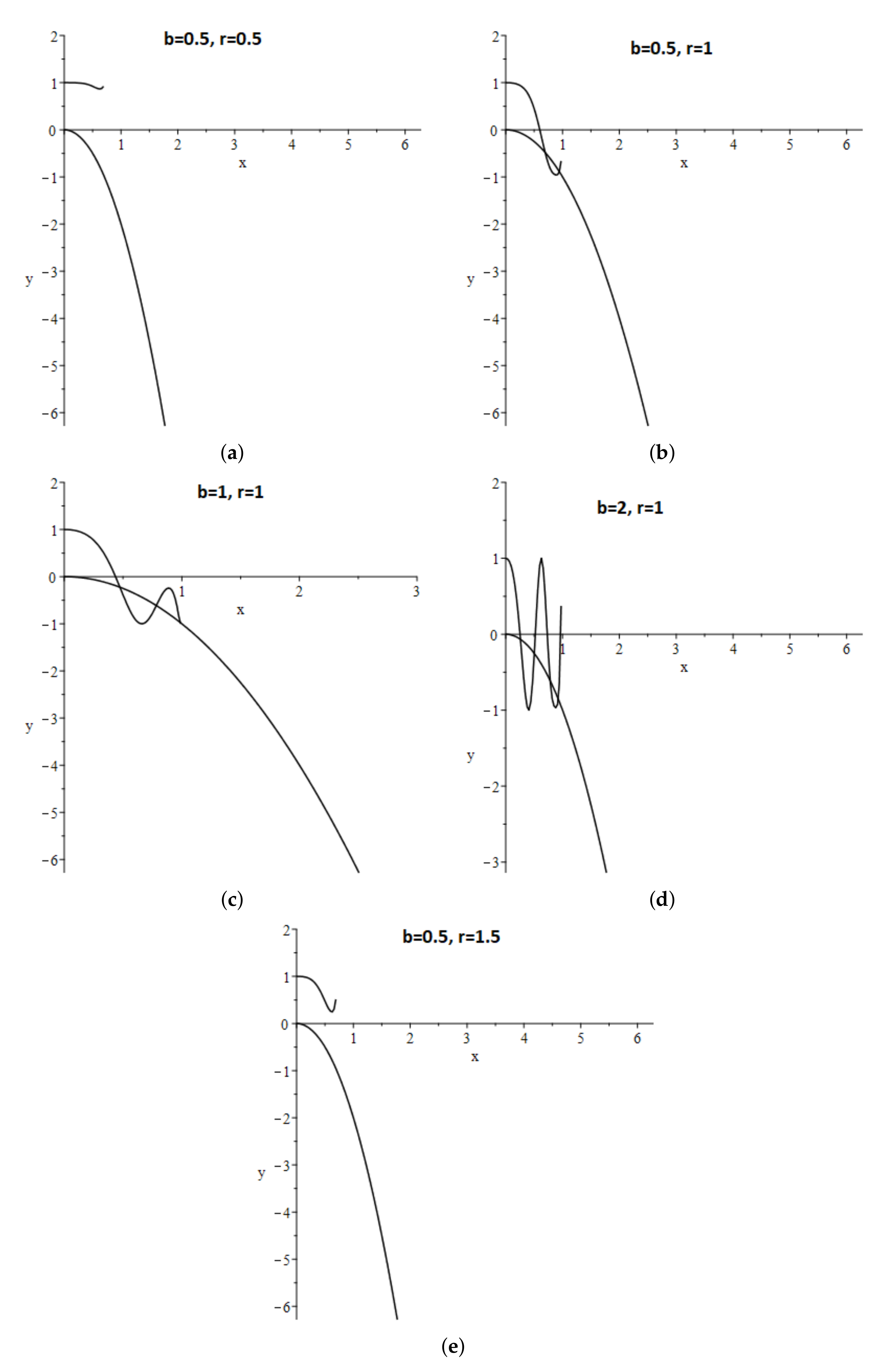
After the roots of this equation have been found for those r and $b_0$ for which they exist, we obtain the desired value $T_0=T_0\left(z_0\right)$. Figure 1 shows the graphs of the left and right sides of Equation (45).

The main difference between the results of this and the previos sections is that $T_0<\frac{\pi }{2r}$ here, and the value $z_0=\epsilon k_{\epsilon }$, at which the critical case is realized, is positive.

We consider a set of integers

$$k_{\epsilon }=z_0{\epsilon }^{-1}+\mathrm{\Theta }+m;m=0,\pm 1,\pm 2,\dots$$

where the quantity $\mathrm{\Theta }=\mathrm{\Theta }\left(\epsilon \right)\in [0,1)$ complements the expression $z_0{\epsilon }^{-1}$ to an integer value. We assume in (40) that $z=z_0+\epsilon (\mathrm{\Theta }+m)$ and let ${\lambda }_m^{+}\left(\epsilon \right)$ and ${\lambda }_m^{-}\left(\epsilon \right)={\overline{\lambda }}_m^{+}\left(\epsilon \right)$ stand for those roots of (40), the real parts of which tend to zero as $\epsilon \to 0$. The following simple statement holds.

Lemma 7.

For ${\lambda }_m^{+}\left(\epsilon \right)$ the asymptotic equalities

$${\lambda }_m^{+}\left(\epsilon \right)=i\omega +\epsilon {\lambda }_{m1}(\mathrm{\Theta }+m)+{\epsilon }^2{\lambda }_{m2}{(\mathrm{\Theta }+m)}^2+\dots$$

hold where

$$\begin{array}{ccc}\hfill {\lambda }_{m1}& =& i{\omega }_1={\lambda }^{\prime }\left(z_0\right),\hfill \\ \hfill {\lambda }_{m2}& =& \frac{1}{2}{\lambda }^{\prime \prime }\left(z_0\right)=\left[1-\frac{1}{2}{T}_0^2{\omega }_1^2(i{b}_0{z}_0-z_0^2-i\omega )\right]·{\left[1-r{T}_{0}exp(-i\omega T_0)\right]}^{-1},\hfill \\ \hfill {\omega }_1& =& i(2z_0+i{b}_0){\left[1+T_0(i\omega +z_0^2-i{b}_0{z}_0)\right]}^{-1},\Im {\omega }_1=0.\hfill \end{array}$$

It is important to note that infinitely many roots of the characteristic Equation (40) tend to imaginary axis as $\epsilon \to 0$. This gives grounds to say that the critical case under consideration has an infinite dimension in the stability problem.

The root ${\lambda }_m^{+}\left(\epsilon \right)$ corresponds to the solution $v_m(t,x,\epsilon )$ of the linearized equation and

$$v_m(t,x,\epsilon )=exp\left(i(z_0{\epsilon }^{-1}+\mathrm{\Theta }+m)x+{\lambda }_m^{+}\left(\epsilon \right)t\right)$$

which means that the same equation has a set of solutions

$$v(t,x,\epsilon )=\sum _{m=-\infty }^{\infty }{\xi }_{m}exp\left(i(z_0{\epsilon }^{-1}+\mathrm{\Theta }+m)x+{\lambda }_m^{+}\left(\epsilon \right)t\right)$$

(46)

where ${\xi }_m$ are arbitrary complex constants. Let $\tau ={\epsilon }^2{t}_0$. Then (46) can be presented in the form

$$\begin{array}{ccc}\hfill v(t,x,\epsilon )& =& exp\left(i(z_0{\epsilon }^{-1}+\mathrm{\Theta })x+i(\omega +\epsilon {\omega }_1\mathrm{\Theta })t\right)·\sum _{m=-\infty }^{\infty }{\xi }_m\left(\tau \right)exp\left(im(x+\epsilon {\omega }_{1}t)\right)\hfill \\ & =& exp\left(i(z_0{\epsilon }^{-1}+\mathrm{\Theta })x+i(\omega +\epsilon {\omega }_1\mathrm{\Theta })t\right)\xi (\tau ,y),y=x+\epsilon {\omega }_{1}t.\hfill \end{array}$$

(47)

Here, we have the equality

$${\xi }_m\left(\tau \right)={\xi }_{m}exp\left(({\lambda }_{m2}+O\left(\epsilon \right))\tau \right)$$

for the Fourier coefficients of the function $\xi (t,y)$.

Further constructions are based on the representation (47).

3.2.2. Construction of Quasinormal Form

For fixed r and $b_0$ and under the conditions (29), (31) we define $\omega ,{\omega }_1,z_0$, and $T_0$. We assume that

$$T=T_0+{\epsilon }^2{T}_1$$

in (27), (28) and let $E=E(t,x,\epsilon )$ stand for the function

$$E=exp\left(i(z_0{\epsilon }^{-1}+\mathrm{\Theta })x+i(\omega +\epsilon \mathrm{\Theta }{\omega }_1)t\right).$$

We introduce into consideration the formal asymptotical series

$$u(t,x,\epsilon )=\epsilon \left(E\xi (\tau ,y)+\overline{E}\overline{\xi }(\tau ,y)\right)+{\epsilon }^2{u}_2+{\epsilon }^3{u}_3+\dots .$$

(48)

Here, $\xi (\tau ,y)$ are the unknown complex amplitudes. The functions $u_j=u_j(t,\tau ,y)$ are $2\pi {\omega }^{-1}$–periodic with respect to t and $2\pi$–periodic with respect to y. We search for solutions of the nonlinear boundary value problem (27), (28) in the form of (48). For this purpose we substitute (48) into (27) and equate the coefficients at the same powers $\epsilon$ in the resulting formal identity. At the first step, we obtain the correct equality by collecting the coefficients at the first power of $\epsilon$. Collecting the coefficients at ${\epsilon }^2$ we obtain the equation for $u_2$. We search for $u_2$ in the form

$$u_2=u_{20}{\left|\xi (\tau ,y)\right|}^2+u_{21}{\xi }^2(\tau ,y)E^2+{\overline{u}}_{21}{\overline{\xi }}^2(\tau ,y){\overline{E}}^2.$$

Then, we immediately get that

$$\begin{array}{ccc}\hfill u_{20}& =& -2z_0^2{r}^{-1},\hfill \\ \hfill u_{21}& =& -rexp(-i\omega T_0){\left[2i\omega +4z_0^2+2i{b}_0{z}_0\right]}^{-1}.\hfill \end{array}$$

At the next step, we obtain the equation for $u_3$:

$$\begin{array}{ccc}\hfill \frac{\partial u_3}{\partial t}& =& {\epsilon }^2\frac{{\partial }^2{u}_3}{\partial x^2}+\epsilon b_0\frac{\partial u_3}{\partial x}-r{u}_3{|}_{t-T,x}\hfill \\ & =& A_0(\tau ,y)+A_1(\tau ,y)E+\overline{cc}+A_2(\tau ,y)E^2+\overline{cc}+A_3(\tau ,y)E^3+\overline{cc},\hfill \end{array}$$

$y=x+2{\omega }_{1}t$. The explicit form of the functions $A_{0,2,3}(\tau ,x)$ is inessential, so we do not write them out. We obtain the formula

$$\begin{array}{ccc}\hfill A_1(\tau ,x)& =& -\frac{\partial \xi }{\partial \tau }+\frac{1}{2}{\lambda }^{\prime \prime }\left(z_0\right){\left(\mathrm{\Theta }+\frac{\partial }{\partial y}\right)}^2\xi +ir\omega T_{1}exp(-i\omega T_0)\xi \hfill \\ & +& {\sigma \xi \left|\xi \right|}^2\left(1-r{T}_{0}exp(-i\omega T_0)\right)\hfill \end{array}$$

for the function $A_1(\tau ,x)$ where

$$\sigma =-r\left[u_{20}+u_{21}(exp\left(i\omega T_0\right)+exp(-2i\omega T_0))\right]{\left(1-r{T}_{0}exp(-i\omega T_0)\right)}^{-1}.$$

The satisfaction of the equality

$$A_1(\tau ,y)\equiv 0$$

is the condition of the solution of the equation for $u_3$ existence in the indicated class of functions, i.e.,

$$\begin{array}{ccc}\hfill \frac{\partial \xi }{\partial \tau }& =& \frac{1}{2}{\lambda }^{\prime \prime }\left(z_0\right)\frac{{\partial }^2\xi }{\partial y^2}+{\lambda }^{\prime \prime }\left(z_0\right)\mathrm{\Theta }\frac{\partial \xi }{\partial y}\hfill \\ & +& \left(\frac{1}{2}{\lambda }^{\prime \prime }\left(z_0\right){\mathrm{\Theta }}^2+ir\omega T_{1}exp(-i\omega T_0)\right)+\sigma \xi {\left|\xi \right|}^2,\xi (\tau ,y+2\pi )\equiv \xi (\tau ,y).\hfill \end{array}$$

(49)

In order to formulate the basic result of this section, we introduce one more notation. Let ${\epsilon }_n\left({\mathrm{\Theta }}_0\right)>0$ stand for the sequence that tend to zero as $n\to \infty$, and the equality

$$\mathrm{\Theta }\left({\epsilon }_n\left({\mathrm{\Theta }}_0\right)\right)={\mathrm{\Theta }}_0$$

holds for all n.

Theorem 4.

Let the conditions (29) and (31) be satisfied. Let $\mathrm{\Theta }={\mathrm{\Theta }}_0$, and let $\xi (\tau ,y)$ be the bounded solution of the boundary value problem (49) as $\tau \to \infty$, $y\in [0,2\pi ]$. Then for $\epsilon ={\epsilon }_n\left({\mathrm{\Theta }}_0\right)$ the function

$$\begin{array}{ccc}\hfill u(t,x,\epsilon )& =& \epsilon \left(E\xi (\tau ,y)+\overline{E}\overline{\xi }(\tau ,y)\right)+{\epsilon }^2(u_{20}{\left|\xi (\tau ,y)\right|}^2+u_{21}{\xi }^2(\tau ,y)E^2\hfill \\ & +& {\overline{u}}_{21}{\overline{\xi }}^2(\tau ,y){\overline{E}}^2),\tau ={\epsilon }^{2}t,y=x+2\epsilon {\omega }_{1}t\hfill \end{array}$$

satisfies the boundary value problem (27), (28) to within $O\left({\epsilon }^3\right)$.

This statement means that in the considered infinite dimensional critical case, the local dynamics of the initial boundary value problem (27), (28) for small $\epsilon$ is determined by the nonlocal behavior of the quasinormal form (49) solutions.

We note that the dynamic properties of (49) may vary for different values of $\mathrm{\Theta }$. This means that an infinite alteration of straight and reverse bifurcations can occur in the initial boundary value problem (27), (28) as $\epsilon \to 0$.

3.3. Quasinormal Forms for Fixed Value $b\ne 0$ and for Sufficiently Small $\epsilon$

In this section, we first define the smallest positive value of the delay coefficient $\tilde{T}$ such that the zero equilibrium state in (27), (28) is asymptotically stable for $T\in (0,\tilde{T})$, but unstable for $T>\tilde{T}$. At the next stage, in the critical case of $T\approx \tilde{T}$, we construct a quasinormal form for the local dynamics study.

It is convenient to perform a change

$$x=y+bt$$

(50)

in (27), (28). As a result, we obtain the boundary value problem with delay and deviation of the spatial variable

$$\frac{\partial u}{\partial t}={\epsilon }^2\frac{{\partial }^{2}u}{\partial y^2}-ru(t-T,y-bT)(1+u),$$

(51)

$$u(t,y+2\pi )\equiv y(t,y).$$

(52)

3.3.1. Linear Analysis

Here, we put

$$T=\epsilon T_0$$

(53)

and show that there exists a value $T_0$ such that for small $\epsilon$ the zero equilibrium state in (51), (52) is asymptotically stable under the condition $0<T<\epsilon T_0$, but unstable for $T>\epsilon T_0$.

Under the condition (53), we consider the characteristic equation for the linearized boundary value problem (51), (52):

$$\lambda =-z^2-rexp\left(-\epsilon T_0\lambda -ib{T}_{0}z\right)$$

(54)

where $z=\epsilon k,k=0,\pm 1,\pm 2,\dots$. For small $\epsilon$, it is natural to start the study with a simpler equation (for $\epsilon T_0=0$)

$$\lambda =-z^2-rexp(-ib{T}_{0}z).$$

(55)

Let $\lambda \left(z_0\right)=i\omega$ for some $z=z_0$ and $\Re \lambda \left(z\right)\le 0$ for all $z\in (-\infty ,\infty )$. Then,

$$\begin{array}{ccc}\hfill -z_0^2& =& rcos\left(b{T}_0{z}_0\right),\omega =rsin\left(b{T}_0{z}_0\right),\hfill \\ \hfill \Re {\lambda }_z^{\prime }\left(z_0\right)& =& -2z_0+rb{T}_{0}sin\left(b{T}_0{z}_0\right)=0.\hfill \end{array}$$

Hence we obtain that for $s=b{T}_0{z}_0$

$$\omega =rsins,coss=-\frac{z_0^2}{r},sins=\frac{2z_0}{rb{T}_0}.$$

Therefore, $tans=-\frac{2}{s}$. Let $s_0$ stand for the smallest positive root of this equation. Then the equality

$$z_0=s_0{\left(b{T}_0\right)}^{-1};z_0=\frac{1}{2}rb{T}_{0}sin{s}_0$$

(56)

holds, which means

$$T_0=b^{-1}{\left(2s_0{(rsin{s}_0)}^{-1}\right)}^{1/2},z_0={\left(-rcos{s}_0\right)}^{1/2}.$$

(57)

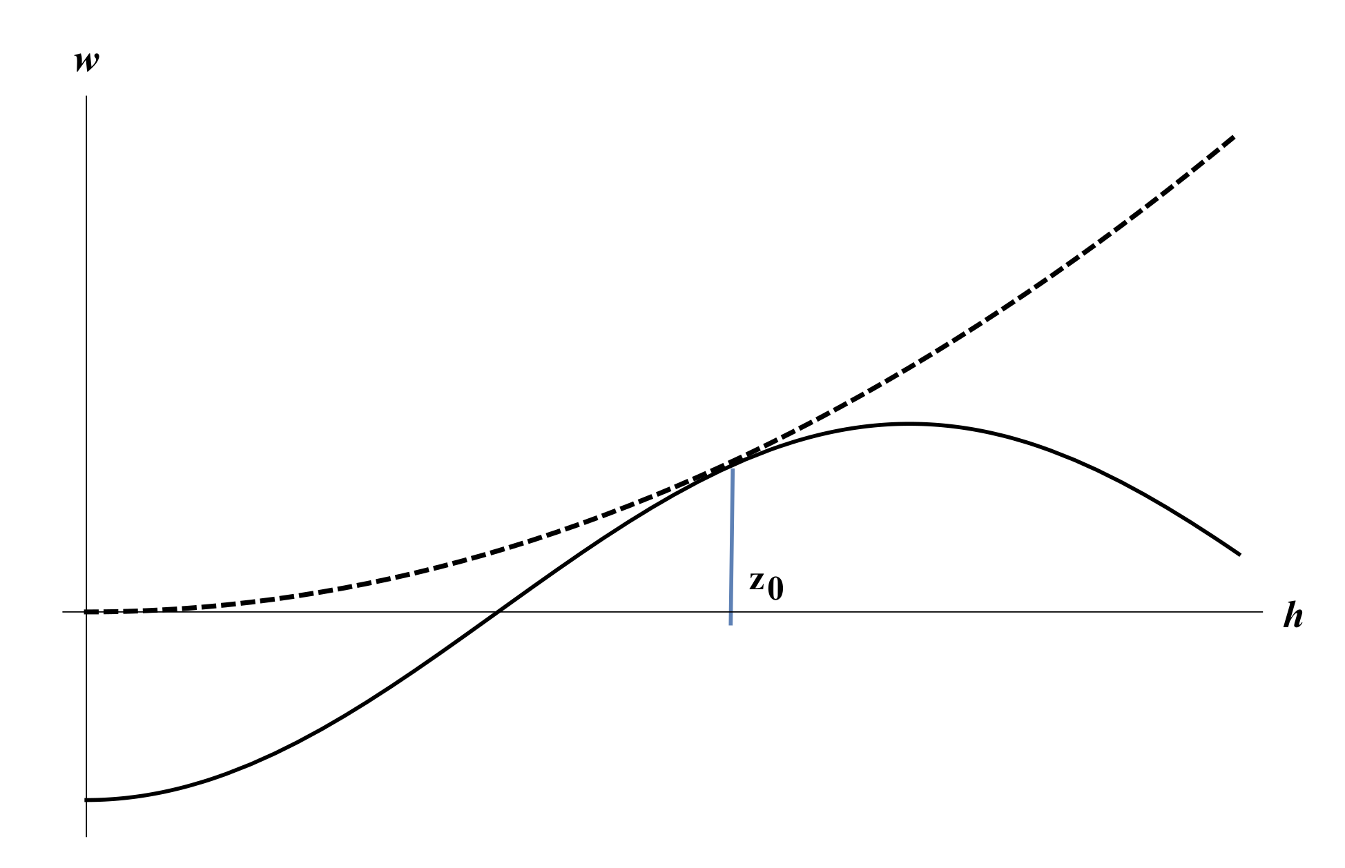
Figure 2 shows the graphs of the functions $w=z^2$ and $w=-rcos\left(b{T}_{0}z\right)$. It is shown that these graphs have tangency at $z=z_0$, i.e., $\Re \lambda \left(z_0\right)=\Re {\lambda }^{\prime }\left(z_0\right)=0$.

At the next stage, we return to the consideration of the characteristic Equation (54). We look for such a value of $T\left(\epsilon \right)$ to within $O\left(\epsilon \right)$ for which the root $\lambda (z,\epsilon )$ of this equation (with the largest real part) satisfies the conditions $\lambda (z_0\left(\epsilon \right),\epsilon )=i\omega \left(\epsilon \right)$, $\Re \lambda (z,\epsilon )\le 0(\forall z)$ and $\Re \frac{d\lambda (z,\epsilon )}{dz}{|}_{z=z_0\left(\epsilon \right)}=0$. Let $T\left(\epsilon \right)=T_0+\epsilon T_1$, $\omega \left(\epsilon \right)=\omega +\epsilon {\omega }_{01}+\dots$, $z_0\left(\epsilon \right)=z_0+\epsilon z_1$. We write out the values $T_1$, ${\omega }_{01}$, and $z_1$. For this purpose, we introduce the $2\times 2$ matrix

$$B=\left(\begin{array}{cc}b{T}_{0}rcos{s}_0-r{z}_0^{-1}sin{s}_0& brsin{s}_0\\ 1-b{T}_0{\left(2z_0\right)}^{-1}rsin{s}_0& -b{z}_0\end{array}\right).$$

We assume $\left(\genfrac{}{}{0.0pt}{}{a_1}{a_2}\right)=B^{-1}\left(\genfrac{}{}{0.0pt}{}{0}{T_0\omega }\right)$. Then $T_1=a_2$, ${\omega }_{01}=r{a}_{1}cos{s}_0$, $z_1=(rasin{s}_0){\left(2z_0\right)}^{-1}$.

Let $\mathrm{\Theta }=\mathrm{\Theta }\left(\epsilon \right)$ complement the expression $z_0{\epsilon }^{-1}+z_1$ to an integer value. Under this condition and for $z=z_0+\epsilon (z_1+\mathrm{\Theta }+m)$, we consider the asymptotics of all those roots ${\lambda }_m^{+}\left(\epsilon \right)(m=0,\pm 1,\pm 2,\dots )$ of Equation (54), whose real parts tend to zero as $\epsilon \to 0$.

We fix arbitrarily the value $T_2$. Let

$$T=T_0+\epsilon T_1+{\epsilon }^2{T}_2.$$

Lemma 8.

The asymptotic equalities

$${\lambda }_m^{+}\left(\epsilon \right)=i\omega +\epsilon {\lambda }_{m1}+{\epsilon }^2{\lambda }_{m2}+\dots$$

hold where

$$\begin{array}{ccc}\hfill {\lambda }_{m1}& =& {\lambda }^{\prime }\left(z_0\right)(z_1+\mathrm{\Theta }+m)=i{\omega }_1(z_1+\mathrm{\Theta }+m),\hfill \\ \hfill {\lambda }_{m2}& =& -d_0{(z_1+\mathrm{\Theta }+m)}^2+d_1(z_1+\mathrm{\Theta }+m)+d_2,\hfill \\ \hfill d_0& =& 1-\frac{1}{2}r{b}^2{T}_0^{2}exp(-ib{T}_0{z}_0),\Re d_0>0,\hfill \\ \hfill d_1& =& i(b{T}_1+T_0{\omega }_1),d_2=irexp\left(ib{T}_0{z}_0\right)(b{T}_2{z}_0+\omega T_1).\hfill \end{array}$$

The set of corresponding to the roots ${\lambda }_m^{+}\left(\epsilon \right)$ solutions of the linearized at zero boundary value problem (27), (28) we write out in the form

$$v(t,x,\epsilon )=\sum _{m=-\infty }^{\infty }{\xi }_{m}exp\left[i\left((z_0+\epsilon z_1){\epsilon }^{-1}+\mathrm{\Theta }+m\right)x+{\lambda }_m^{+}\left(\epsilon \right)t\right]=E\xi (\tau ,y)$$

(58)

where $\tau ={\epsilon }^{2}t$, and $y=x+\epsilon {\omega }_{1}t$, ${\xi }_m\left(\tau \right)={\xi }_{m}exp\left(({\lambda }_{m2}+O\left(\epsilon \right))\tau \right)$ are the Fourier coefficients of the function $\xi (\tau ,y)$.

3.3.2. Nonlinear Analysis

In the case under consideration, the formal representation of the nonlinear boundary value problem (27), (28) solutions is based on formula (58) for the linearized problem solutions. Therefore, we introduce into consideration the asymptotic expression

$$u(t,x,\epsilon )=\epsilon \left(E\xi (\tau ,y)+\overline{E}\overline{\xi }(\tau ,y)\right)+{\epsilon }^2{u}_2+{\epsilon }^3{u}_3+\dots$$

(59)

to construct a quasinormal form.

As in Section 3.2.2, we obtain here

$$\begin{array}{ccc}\hfill u_2& =& u_{20}{\left|\xi (\tau ,y)\right|}^2+u_{21}{\xi }^2(\tau ,y)E^2+{\overline{u}}_{21}{\overline{\xi }}^2(\tau ,y){\overline{E}}^2,\hfill \\ \hfill u_3& =& u_{30}(\tau ,y)+u_{31}(\tau ,y)E+\overline{cc}+u_{32}(\tau ,y)E^2+\overline{cc}+u_{33}(\tau ,y)E^3+\overline{cc}.\hfill \end{array}$$

Substituting (59) into (27) and performing standard operations, we obtain the equalities

$$\begin{array}{ccc}\hfill u_{20}& =& -2cos\left(b{T}_0{z}_0\right){\left|\xi (\tau ,y)\right|}^2,\hfill \\ \hfill u_{21}& =& r{\left[2i\omega +4z_0^2+rexp(-2ib{T}_0{z}_0)\right]}^{-1}{\xi }^2(\tau ,y)\hfill \end{array}$$

first. At the next step, we get the equation for $u_3$. Expressions for $u_{30}$, $u_{32}$, and $u_{33}$ are simply defined, and the condition of solvability of the equation for $u_{31}$ leads to the relations

$$\frac{\partial \xi }{\partial \tau }=d_0\frac{{\partial }^2\xi }{\partial y^2}-i(2d_0+d_1)(z_1+\mathrm{\Theta })\frac{\partial \xi }{\partial y}+\left(d_2+d_1(z_1+\mathrm{\Theta })-d_2{(z_1+\mathrm{\Theta })}^2\right)\xi +\delta \xi {\left|\xi \right|}^3,$$

(60)

$$\xi (\tau ,y+2\pi )\equiv \xi (\tau ,y).$$

(61)

For the value $\delta$ the equality

$$\delta =-r{u}_{20}(1+exp(-ib{T}_0{z}_0))-r{u}_{21}(exp(-2ib{T}_0{z}_0)+exp\left(ib{T}_0{z}_0\right))$$

holds. The next statement follows from the above constructions.

Theorem 5.

Let the parameters $b\ne 0$ and ${\mathrm{\Theta }}_0$ be fixed, and the values $z_0$ and $T_0$ are defined. Let $\xi (\tau ,y)$ be the bounded for $\tau \to \infty$, $y\in [0,2\pi ]$ solution of the boundary value problem (60), (61) as $\mathrm{\Theta }={\mathrm{\Theta }}_0$. Then for $\epsilon ={\epsilon }_n\left({\mathrm{\Theta }}_0\right)$ the function

$$u(t,x,\epsilon )=\epsilon \left(E\xi (\tau ,y)+\overline{E}\overline{\xi }(\tau ,y)\right)+{\epsilon }^2\left(u_{20}{\left|\xi (\tau ,y)\right|}^2+u_{21}{\xi }^2(\tau ,y)E^2+{\overline{u}}_{21}{\overline{\xi }}^2(\tau ,y){\overline{E}}^2\right)$$

satisfies the boundary value problem (27), (28) to within $O\left({\epsilon }^3\right)$ as $\tau ={\epsilon }^{2}t$, $y=x+\epsilon {\omega }_{1}t$.

Due to the parabolicity condition $\Re d_0>0$, the boundary value problem (60), (61) is the Ginzburg–Landau equation.

3.4. Quasinormal Form in the Case of Low Diffusion and Large Translation Coefficient

This case is simpler than the one discussed in the previous section.

Let $b\gg 1$, i.e., the parameter $\mu =b^{-1}$ satisfies the condition

$$0<\mu \ll 1.$$

In this case, the threshold value of the parameter T is determined by the condition

$$T=\epsilon \mu T_0.$$

(62)

This means that it is an order of magnitude less than in (53). Then, the characteristic equation has the form

$$\lambda =-z^2-rexp\left[-\epsilon \mu T_0\lambda -i{T}_{0}z\right].$$

(63)

The equation of first approximation

$$\lambda =-z^2-rexp[-i{T}_{0}z]$$

defines the behavior of the roots (63) with higher precision (compared to (54)) near the imaginary axis. The formulas (56) and (57) in which the parameter b should be replaced by 1 are correct. The resulting quasinormal form coincides with (60), (61) for $b=1$, $T_1=z_1=0$.

3.5. On Dynamics of Delay Logistic Equation with Small Diffusion and Classical Boundary Conditions of General Form

We consider the problem of the local dynamics of the delay logistic equation with small coefficients of diffusion and advection

$$\frac{\partial u}{\partial t}={\epsilon }^2\frac{{\partial }^{2}u}{\partial x^2}+{\epsilon }^{2}b\frac{\partial u}{\partial x}-ru(t-T,x)[1+u],x\in [0,1]$$

(64)

with the boundary conditions

$$\frac{\partial u}{\partial x}{|}_{x=0}={\gamma }_{1}u{|}_{x=0},\frac{\partial u}{\partial x}{|}_{x=1}={\gamma }_{2}u{|}_{x=1}.$$

(65)

All coefficients in (64), (65) are real, $r>0$, $T>0$, and $\epsilon$ is a small positive parameter:

$$0<\epsilon \ll 1.$$

(66)

The construction of the characteristic equation for the linearized at zero boundary value problem

$$\frac{\partial v}{\partial t}={\epsilon }^2\frac{{\partial }^{2}v}{\partial x^2}+{\epsilon }^{2}b\frac{\partial v}{\partial x}-rv(t-1,x),$$

(67)

$$\frac{\partial v}{\partial x}{|}_{x=0}={\gamma }_{1}v{|}_{x=0},\frac{\partial v}{\partial x}{|}_{x=1}={\gamma }_{2}v{|}_{x=1}$$

(68)

is related to the eigenvalues of the stationary boundary value problem

$$\frac{d^2\phi }{d{x}^2}+b\frac{d\phi }{dx}=\mu \phi ,{\phi }^{\prime }\left(0\right)={\gamma }_1\phi \left(0\right),{\phi }^{\prime }\left(1\right)={\gamma }_2\phi \left(1\right).$$

(69)

All eigenvalues ${\mu }_j(j=0,1,\dots )$ of this boundary value problem are real and can be arranged in descending order. The corresponding to ${\mu }_j$ eigenfunctions ${\phi }_j\left(x\right)$ are also real. We note that they form a complete set in the corresponding space.

We consider the question of the roots of the quasipolynomial

$$\lambda +rexp(-\lambda T)={\epsilon }^2{\mu }_j$$

(70)

for each number j. Here are some standard statements.

Lemma 9.

Let $0<r<\frac{\pi }{2}$. Then, for all sufficiently small ε, the real parts of Equation (70) roots are negative and separated from zero as $\epsilon \to 0$.

Lemma 10.

Let $r>\frac{\pi }{2}$. Then, for all sufficiently small ε, Equation (70) has a root with positive and separated from zero real part as $\epsilon \to 0$.

Lemma 11.

Equation (70) has a pair of complex roots ${\lambda }_j^{\pm }\left(\epsilon \right)\left({\lambda }_j^{-}\left(\epsilon \right)={\overline{\lambda }}_j^{+}\left(\epsilon \right)\right)$ for each $j=0,1,2,\dots$ and

$${\lambda }_j^{+}\left(\epsilon \right)=i\pi {\left(2T\right)}^{-1}+{\epsilon }^2{\lambda }_{j1}+\dots ,{\lambda }_{j1}=T^{-1}\left(1-i\frac{\pi }{2}{\mu }_j\right).$$

All other roots of this equation have negative real parts and are separated from zero as $\epsilon \to 0$.

Below we assume that the equality

$$r=\frac{\pi }{2}+{\epsilon }^2{r}_1$$

(71)

holds for an arbitrarily fixed value $r_1$.

The linear boundary value problem (67), (68) has a set of solutions

$$v=\left(\sum _{j=0}^{\infty }{c}_j{\phi }_j\left(x\right)exp\left(({\lambda }_{j1}+o\left(\epsilon \right))\tau \right)\right)exp\left(i\pi {\left(2T\right)}^{-1}t\right)=\xi (\tau ,x)exp\left(i\pi {\left(2T\right)}^{-1}t\right)$$

where $c_j$ are arbitrary, and the Fourier coefficients $c_j(\tau ,x)$ of the function $\xi (\tau ,x)$ have the form $c_j(\tau ,x)=c_{j}exp\left(({\lambda }_{j1}+o\left(\epsilon \right))\tau \right)$.

Based on this representation of ‘critical’ solutions of the linear problem (67), (68), we look for the nonlinear boundary value problem (64), (65) solutions in the form

$$u=\epsilon \left(\xi (\tau ,x)exp\left(i\pi {\left(2T\right)}^{-1}t\right)+\overline{cc}\right)+{\epsilon }^2{u}_2(t,\tau ,x)+\dots .$$

(72)

Here and below, let $\overline{cc}$ stand for the expression that is a complex conjugate to the previous term. The unknown function $\xi (\tau ,x)$ is sufficiently smooth and satisfies the boundary conditions (65). The dependence on the argument t on the right-hand side of (72) is $4T$–periodic.

We substitute expression (72) into (64) and collect the coefficients at the same powers of $\epsilon$. We obtain the correct equality for the first degree of $\epsilon$. At the next step, we obtain the equation

$$\frac{\partial u_2}{\partial t}=-r{u}_2(t-T,x)-rexp\left(-i\frac{\pi }{2}\right){\xi }^2(\tau ,x)exp\left(i\pi T^{-1}t\right)+\overline{cc}$$

for $u_2$. From this we find that

$$u_2=u_{20}{\xi }^{2}exp\left(i\pi T^{-1}t\right),u_{20}=ir{\left[i\pi T^{-1}-r\right]}^{-1}.$$

(73)

However, the boundary conditions (65) for the function $u_2$, generally speaking, are not satisfied. In order to satisfy these boundary conditions for the terms of ${\epsilon }^2$ order, we look for the expression for ${\epsilon }^3$ in (72) in the form

$$u_3=u_3(t,\tau ,x)+w_{31}(t,\tau ,y_1)+w_{32}(t,\tau ,y_2)$$

(74)

where $y_1=x{\epsilon }^{-1}$, $y_2=(1-x){\epsilon }^{-1}$. All functions are $4T$–periodic with respect to the variable t, and each of the functions $w_{31}$ and $w_{32}$ is exponentially decreasing with respect to its third argument: for some $p_0>0$ and $c_0>0$ the evaluations

$$\left|w_{3j}(t,\tau ,y_j)\right|\le c_{0}exp(-p_0{y}_j),(j=1,2)$$

(75)

are satisfied. We substitute

$$u=\epsilon \left(\xi exp\left(i\pi {\left(2T\right)}^{-1}t\right)+\overline{cc}\right)+{\epsilon }^2{u}_2+{\epsilon }^3(u_3+w_{31}+w_{32})$$

(76)

into (64), (65). Then, we obtain the relations

$$\frac{\partial u_2}{\partial x}{|}_{x=0}+\frac{\partial w_{31}}{\partial y_1}{|}_{y_1=0}={\gamma }_1{u}_2{|}_{x=0},\frac{\partial u_2}{\partial x}{|}_{x=1}+\frac{\partial w_{32}}{\partial y_2}{|}_{y_2=0}={\gamma }_2{u}_2{|}_{x=1}$$

(77)

for the degree ${\epsilon }^2$ in the boundary conditions (65). Taking into account equality (73) here, we find that

$$\frac{\partial w_{31}}{\partial y_1}{|}_{y_1=0}=u_{20}exp\left(i\pi T^{-1}t\right)\left[{\gamma }_1{\xi }^2{|}_{x=0}-2\xi {|}_{x=0}\frac{\partial \xi }{\partial x}{|}_{x=0}\right]+\overline{cc},$$

(78)

$$\frac{\partial w_{32}}{\partial y_2}{|}_{y_2=0}=u_{20}exp\left(i\pi T^{-1}t\right)\left[{\gamma }_2{\xi }^2{|}_{x=1}-2\xi {|}_{x=1}\frac{\partial \xi }{\partial x}{|}_{x=1}\right]+\overline{cc}.$$

(79)

We take one more step. We write down the relation for the coefficients of ${\epsilon }^3$ that is obtained after substituting (74) into (64):

$$\begin{array}{c}\frac{\partial u_3}{\partial t}+\frac{\partial w_{31}}{\partial t}+\frac{\partial w_{32}}{\partial t}+r\left(u_3(t-1,x)+w_{31}(t-1,\tau ,y_1)+w_{32}(t-1,\tau ,y_2)\right)\hfill \\ \hfill =B_{1}exp\left(i\pi {\left(2T\right)}^{-1}t\right)+\overline{cc}+B_{3}exp\left(3i\pi {\left(2T\right)}^{-1}t\right)+\overline{cc}.\end{array}$$

(80)

Here the following notation is adopted:

$$\begin{array}{ccc}\hfill B_1& =& -(1-ir)\frac{\partial \xi }{\partial \tau }+\frac{{\partial }^2\xi }{\partial x^2}+b\frac{\partial \xi }{\partial x}+i{r}_1\xi +r(1-i)u_{20}\xi {\left|\xi \right|}^2,\hfill \\ \hfill B_3& =& r(1+i)u_{20}{\xi }^3.\hfill \end{array}$$

It is natural to look for the functions appearing in (80) in the form

$$u_3=u_{31}exp\left(i\pi {\left(2T\right)}^{-1}t\right)+\overline{cc}+u_{33}exp\left(3i\pi {\left(2T\right)}^{-1}t\right)+\overline{cc},$$

(81)

$$w_{31}=w_{31}^{\circ }exp\left(2i\pi {\left(2T\right)}^{-1}t\right)+\overline{cc},$$

(82)

$$w_{32}=w_{32}^{\circ }exp\left(2i\pi {\left(2T\right)}^{-1}t\right)+\overline{cc}.$$

(83)

Then, from the Equation (80) we arrive at the system of four equations

$$B_1=0,$$

(84)

$$\left[3i\pi {\left(2T\right)}^{-1}+rexp\left(-3i\pi {\left(2T\right)}^{-1}\right)\right]u_{33}=B_3,$$

(85)

$$\left[i\pi T^{-1}+rexp\left(-i\pi T^{-1}\right)\right]w_{3j}^{\circ }+\frac{{\partial }^2{w}_{31}^{\circ }}{\partial y_j^2}=0,(j=1,2).$$

(86)

We conclude from (81) that

$$\frac{\partial \xi }{\partial \tau }={(1-ir)}^{-1}\left[\frac{{\partial }^2\xi }{\partial x^2}+b\frac{\partial \xi }{\partial x}+i{r}_1\xi +{\sigma }_0\xi {\left|\xi \right|}^2\right],$$

(87)

$$\frac{\partial \xi }{\partial x}{|}_{x=0}={\gamma }_1\xi {|}_{x=0},\frac{\partial \xi }{\partial x}{|}_{x=1}={\gamma }_2\xi {|}_{x=1}.$$

(88)

We obtain from (82) that

$$u_{33}=C{\xi }^3$$

(89)

and

$$C={\left[3i\pi {\left(2T\right)}^{-1}+rexp\left(-3i\pi {\left(2T\right)}^{-1}\right)\right]}^{-1}·r(1+i)u_{20}.$$

(90)

From (83) and conditions (75), (78), (79) we obtain that

$$w_{3j}^{\circ }=C_{j}exp\left({\delta }_0{y}_j\right),(j=1,2),$$

(91)

$$C_1=u_{20}\left[{\gamma }_1{\xi }^2{|}_{x=0}-2\xi {|}_{x=0}{\frac{\partial \xi }{\partial x}}_{x=0}\right],$$

(92)

$$C_2=u_{20}\left[{\gamma }_1{\xi }^2{|}_{x=1}-2\xi {|}_{x=1}{\frac{\partial \xi }{\partial x}}_{x=1}\right].$$

(93)

We denote by ${\delta }_0$ one of ${\left(i\pi T^{-1}+rexp\left(-i\pi T^{-1}\right)\right)}^{1/2}$ roots, whose real part is negative.

We summarize with the following statement.

Theorem 6.

Let the condition (71) be satisfied, and let $\xi (\tau ,x)$ be a bounded for $\tau \to \infty$, $x\in [0,1]$ solution of the boundary value problem (87), (88). Let $\tau ={\epsilon }^{2}t$, $y_1=x{\epsilon }^{-1}$, $y_2=(1-x){\epsilon }^{-1}$, and the function $u_2$ is defined in (73), the function $u_3$ is defined in (81)–(83) and in (90)–(93). Then, the function (76) satisfies Equation (64) to within $O\left({\epsilon }^4\right)$, and satisfies the boundary conditions (65) to within $O\left({\epsilon }^3\right)$.

We make one remark. The algorithm presented here for constructing the asymptotics of the boundary value problem (64), (65) solution can be continued indefinitely.

4. About Infinite-Dimensional Bifurcations in the Case of Large Delay and Dirichlet Boundary Conditions

We note that the zero solution of the boundary value problem (1), (2) is unstable for sufficiently large values of the delay parameter T. However, the relaxation cycle is stable [15] in this case. Its asymptotic behavior is given in [15].

The local behavior of the (1), (2) solutions under other classical boundary conditions is determined by the roots of its characteristic equation for the linearized at zero boundary value problem. Some results for such cases are presented in [25].

4.1. Case of $b=0$

First, we dwell on the simplest case of $b=0$. We replace u by $u-1$ and consider Equation (1) with the Dirichlet boundary conditions

$$\frac{\partial u}{\partial t}=d\frac{{\partial }^{2}u}{\partial x^2}-ru(t-T,x)[1+u],u(t,0)=u(t,1)=0.$$

(94)

Its characteristic equation coincides with (10) but the values of the integers k are only the following: $k=1,2,\dots$:

$$\lambda =-d{\pi }^2{k}^2-rexp(-\lambda T).$$

We analyse its roots. The roots of this equation have negative real parts for $T>0$ as $0<r<d$. Let the condition $r=r_0$ be satisfied where

$$r_0=d{\pi }^2.$$

The basic assumption of this section is that $T\gg 1$, i.e.,

$$\epsilon =T^{-1},0<\epsilon \ll 1.$$

(95)

The dynamics of the solutions of the delay equations under the condition $T\gg 1$ was studied in [26,27].

It is convenient to make the substitution $t=T{t}_1$ in (94). Consequently, we obtain the singularly perturbed boundary value problem:

$$\epsilon \frac{\partial u}{\partial t}=d\frac{{\partial }^{2}u}{\partial x^2}-ru(t-1,x)[1+u],u(t,0)=u(t,1)=0.$$

(96)

Here, we omit the index 1 for $t_1$, and the characteristic equation for the boundary value problem (96), which is linearized on $u_0\equiv 1$ takes the form

$$\epsilon \lambda =-d{\pi }^2{k}^2-rexp(-\lambda ).$$

(97)

We investigate the behavior of the boundary value problem (96) solutions in the zero equilibrium neighborhood under the condition (95) as

$$r=r_0+{\epsilon }^2{r}_1$$

(98)

where $r_1$ is arbitrarily fixed.

The next statement shows that the critical case of infinite dimension is realized in the boundary value problem (96).

Lemma 12.

Under the conditions (95), (98), the characteristic Equation (97) has no roots with positive and separated from zero real part but has infinitely many roots ${\lambda }_m^{\pm }\left(\epsilon \right)\left({\lambda }_m^{-}\left(\epsilon \right)={\overline{\lambda }}_m^{+}\left(\epsilon \right)\right)m=0,$ $\pm 1,\pm 2,\dots$ which tend to the imaginary axis for each m as $\epsilon \to 0$, and the asymptotic equalities

$$\begin{array}{ccc}\hfill {\lambda }_m^{+}\left(\epsilon \right)& =& i\pi (2m+1)+\epsilon {\lambda }_{m1}+{\epsilon }^2{\lambda }_{m2}+\dots ,\hfill \\ \hfill {\lambda }_{m1}& =& -i{d}^{-1}\pi (2m+1),\hfill \\ \hfill {\lambda }_{m2}& =& -d^{-2}{\pi }^2{(2m+1)}^2+i{d}^{-2}\pi (2m+1)+r_1\hfill \end{array}$$

hold.

We note that the solutions of (94) are unstable for $r>d{\pi }^2$ and for sufficiently large T.

The solution of the linearized equation

$$v_m(t,x,\epsilon )=sin\pi x·exp\left({\lambda }_m\left(\epsilon \right)t\right)$$

corresponds to the root ${\lambda }_m^{+}\left(\epsilon \right)$. The set of the solutions $v(t,x,\epsilon )={\displaystyle \sum _{m=-\infty }^{\infty }}{\xi }_m{v}_m(t,x,\epsilon )$ can be represented as

$$v(t,x,\epsilon )=sin\pi x·\xi (\tau ,y).$$

Here $\tau ={\epsilon }^{2}t$, $y=(1-\epsilon {\left(d{r}_0\right)}^{-1})t$, the function $\xi (\tau ,y)$ is 1–antiperiodic with respect to y: $\xi (\tau ,y+1)\equiv -\xi (\tau ,y)$. Its Fourier coefficients with respect to the variable y satisfy the formula

$${\xi }_m\left(\tau \right)={\xi }_{m}exp\left(({\lambda }_{m2}+o\left(\epsilon \right))\tau \right).$$

According to the technique from the previous sections, we seek the solutions of the nonlinear boundary value problem (97) in the neighborhood of $u_0\equiv 0$ in the form

$$u(t,x,\epsilon )={\epsilon }^{\frac{1}{2}}sin\pi x·\xi (\tau ,y)+\epsilon u_2(\tau ,x,y)+{\epsilon }^{\frac{5}{2}}{u}_3(\tau ,x,y)+\dots .$$

(99)

For the sequential finding of the elements of the formal series (99), we substitute (99) into (96) and perform standard actions.

First, we obtain the equation

$$d\frac{{\partial }^2{u}_2}{\partial x^2}-d{\pi }^2{u}_2=d{\pi }^2{\xi }^2(\tau ,y){sin}^2\pi x,{\left.u_2\right|}_{x=0}={\left.u_2\right|}_{x=1}=0$$

for $u_2$. It follows that

$$\begin{array}{ccc}\hfill u_2(\tau ,x,y)& =& d{\pi }^2{\xi }^2(\tau ,y)p\left(x\right),\hfill \\ \hfill p\left(x\right)& =& \left[-\frac{1}{2}+\frac{1}{10}cos2\pi x+\frac{2}{5}coth\pi x-\frac{2}{5}(1-coth\pi ){(sinh\pi )}^{-1}\right].\hfill \end{array}$$

At the next step, we obtain the boundary value problem

$$\begin{array}{ccc}\hfill d\frac{{\partial }^2{u}_3}{\partial x^2}-d{\pi }^2{u}_3& =& \left[\frac{\partial \xi }{\partial \tau }-r_1\xi \right.\hfill \\ & -& \left.\frac{1}{2d^2}\frac{{\partial }^2\xi }{\partial y^2}-dp\left(x\right){\xi }^2\frac{\partial \xi }{\partial y}\right]{sin}^2\pi x,{\left.u_3\right|}_{x=0}={\left.u_3\right|}_{x=1}=0\hfill \end{array}$$

(100)

for $u_3$. For the existence of this boundary value problem solution, it is necessary and sufficient that

$$\frac{\partial \xi }{\partial \tau }={\left(2d^2\right)}^{-1}\frac{{\partial }^2\xi }{\partial y^2}+r_1\xi +\gamma {\xi }^2\frac{\partial \xi }{\partial y},\xi (\tau ,y+1)\equiv -\xi (\tau ,y)$$

(101)

where $\gamma =d\underset{0}{\overset{1}{\int }}p\left(x\right){sin}^2\pi xdx$. We do not present an explicit formula for $\gamma$ due to its inconvenience. We only note that $\gamma <0$. Hence the statement follows.

Theorem 7.

Let the conditions (95), (98) be satisfied and the boundary value problem (101) has the bounded for $\tau \to \infty$, $y\in [0,2]$ solution $\xi (\tau ,y)$. Then for $\tau ={\epsilon }^{2}t$, $y=(1-\epsilon d^{-1})t$ the function

$$u(t,x,\epsilon )={\epsilon }^{\frac{1}{2}}\xi (\tau ,y)sin\pi x+\epsilon {\xi }^2(\tau ,y)p\left(x\right)$$

satisfies the boundary value problem (96) to within $O\left({\epsilon }^2\right)$.

Thus, the boundary value problem (101) is a quasinormal form for the boundary value problem (96). In contrast to the previously presented quasinormal forms, its coefficients here are real.

4.2. Case of $b\ne 0$

After the replacement (95) in the boundary value problem

$$\frac{\partial u}{\partial t}=d\frac{{\partial }^{2}u}{\partial x^2}+b\frac{\partial u}{\partial x}=ru(t-T,x)[1+u],u(t,0)=u(t,1)=0$$

we obtain the following boundary value problem

$$\epsilon \frac{\partial u}{\partial t}=d\frac{{\partial }^{2}u}{\partial x^2}+b\frac{\partial u}{\partial x}-ru(t-1,x)[1+u],u(t,0)=u(t,1)=0.$$

(102)

To obtain the characteristic equation, we first linearize this boundary value problem at zero and then set $u=vexp\lambda t$. Then we obtain the equation

$$d\frac{d^{2}v}{d{x}^2}+b\frac{dv}{dx}-(\epsilon \lambda +rexp(-\lambda ))v=0$$

(103)

with the boundary conditions

$$v\left(0\right)=v\left(1\right)=0.$$

(104)

After the replacement

$$v=exp\left(-\frac{b}{2}x\right)W$$

in (103) we obtain the equation with the Dirichlet boundary conditions

$$d\frac{d^{2}W}{d{x}^2}-\left[b^2{\left(4d\right)}^{-1}+\epsilon \lambda +rexp(-\lambda )\right]W=0,W\left(0\right)=W\left(1\right)=0.$$

Hence, we conclude that

$$\epsilon \lambda +rexp(-\lambda )=-{\pi }^{2}d{k}^2-b^2{\left(4d\right)}^{-1},k=1,2,\dots .$$

(105)

Now we formulate an assertion about the roots of this equation.

Lemma 13.

Under the condition $0<r<d{\pi }^2+b^2{\left(4d\right)}^{-1}$ and for sufficiently small ε, the roots of (105) have negative and separated from zero real parts as $\epsilon \to 0$. If $r>d{\pi }^2+b^2{\left(4d\right)}^{-1}$ then Equation (105) has a root with a positive real part separated from zero as $\epsilon \to 0$.

The critical case is realized for $r=r_0$ where

$$r_0=d{\pi }^2+b^2{\left(4d\right)}^{-1}.$$

Under this condition and (98), infinitely many roots ${\lambda }_m^{\pm }\left(\epsilon \right)$ in (103) tend to the imaginary axis as $\epsilon \to 0$, and the asymptotic equalities

$${\lambda }_m^{+}\left(\epsilon \right)=i\pi (2m+1)+\epsilon {\lambda }_{m1}+{\epsilon }^2{\lambda }_{m2}+\dots$$

hold. Here $m=0,\pm 1,\pm 2,\dots ,$

$$\begin{array}{ccc}\hfill {\lambda }_{m1}& =& -\pi (2m+1)i{r}_0^{-1},\hfill \\ \hfill {\lambda }_{m2}& =& -{\pi }^2{(2m+1)}^2{\left(2r_0\right)}^{-1}-i\pi (2m+1){\left(r_0^2\right)}^{-1}+r_1{r}_0^{-1}.\hfill \end{array}$$

The root ${\lambda }_m^{+}\left(\epsilon \right)$ corresponds to the solution of the linearized equation

$$v_m(t,x,\epsilon )=sin\left(\pi x\right)·exp\left(-\frac{b}{2d}x\right)exp\left({\lambda }_m\left(\epsilon \right)t\right).$$

Repeating the scheme from Section 4.1, we consider the formal series

$$u(t,x,\epsilon )={\epsilon }^{\frac{1}{2}}sin\left(\pi x\right)exp\left(-\frac{b}{2d}x\right)\xi (\tau ,y)+\epsilon u_2(\tau ,x,y)+{\epsilon }^{\frac{5}{2}}{u}_3(\tau ,x,y)+\dots$$

(106)

where $\tau ={\epsilon }^{2}t$, $y=\left(1-\epsilon {\left(d{r}_0\right)}^{-1}\right)t$. The function $\xi (\tau ,y)$ is 1–antiperiodic with respect to y:

$$\xi (\tau ,y+1)\equiv -\xi (\tau ,y).$$

(107)

The functions $u_{2,3}(\tau ,x,y)$ are periodic with respect to x and y. We substitute (106) into (102). Performing standard actions, we obtain the boundary value problem

$$d\frac{{\partial }^2{u}_2}{\partial x_2}+b\frac{\partial u_2}{\partial x}+r_0{u}_2=r_0{\xi }^2(\tau ,y){sin}^2\pi x·exp\left(-\frac{b}{d}x\right),$$

(108)

$$u_2(\tau ,0,y)=u_2(\tau ,1,y)=0$$

(109)

for $u_2$. For simplicity, we assume that $4d{r}_0\ne b$. It follows that the equation $d{\lambda }^2+b\lambda +r_0=0$ has simple roots ${\lambda }_1$ and ${\lambda }_2$. From (108), (109) we obtain that

$$u_2(\tau ,x,y)=r_0{\xi }^2(\tau ,y)P\left(x\right)$$

where

$$\begin{array}{ccc}\hfill P\left(x\right)& =& {(exp{\lambda }_1-exp{\lambda }_2)}^{-1}\underset{0}{\overset{x}{\int }}K(x-s){sin}^2\pi s·exp\left(-\frac{b}{d}s\right)ds,\hfill \\ \hfill K\left(x\right)& =& {({\lambda }_1-{\lambda }_2)}^{-1}\left(exp\left({\lambda }_{1}x\right)-exp\left({\lambda }_{2}x\right)\right).\hfill \end{array}$$

At the next step, we obtain the boundary value problem

$$\begin{array}{ccc}\hfill d\frac{{\partial }^2{u}_3}{\partial x^2}+b\frac{\partial u_3}{\partial x}-r_0{u}_3& =& \left[(1+r_0)\frac{\partial \xi }{\partial \tau }-\frac{1}{2}{\left(d{r}_0\right)}^{-2}\frac{{\partial }^2\xi }{\partial y^2}-r_1\xi +\right.\hfill \\ & +& \left.dp\left(x\right){\xi }^2\frac{\partial \xi }{\partial y}\right]sin\pi x·exp\left(-\frac{b}{2d}x\right),{\left.u_3\right|}_{x=0}={\left.u_3\right|}_{x=1}=0\hfill \end{array}$$

to find $u_3$.

The equality to zero of the integral with respect to x from 0 to 1 from the right-hand side is the condition for the existence of a solution of this boundary value problem with respect to $u_3$. Hence, we conclude that the function $\xi (\tau ,y)$ is a solution of the boundary value problem

$$(1+r_0)\frac{\partial \xi }{\partial \tau }=\frac{1}{2}{\left(d{r}_0\right)}^{-2}\frac{{\partial }^2\xi }{\partial y^2}+r_1\xi +{\gamma }_0{\xi }^2\frac{\partial \xi }{\partial y},\xi (\tau ,y+1)\equiv -\xi (\tau ,y)$$

where ${\gamma }_0=d\underset{0}{\overset{1}{\int }}p\left(x\right){sin}^2\pi xdx$. Theorem 7 holds for this boundary value problem.

4.3. Extending the Results to Other Boundary Conditions

As an example, we consider the boundary value problem

$$\epsilon \frac{\partial u}{\partial t}=d\frac{{\partial }^{2}u}{\partial x^2}+b\frac{\partial u}{\partial x}-ru(t-1,x)[1+u]$$

(110)

with the boundary conditions

$$\frac{\partial u}{\partial x}{|}_{x=0}={\gamma }_{1}u{|}_{x=0},\frac{\partial u}{\partial x}{|}_{x=1}={\gamma }_{2}u{|}_{x=1}.$$

(111)

Here all the coefficients are real. We agree to assume that the notation ${\gamma }_1=\infty$ corresponds to the boundary condition ${\left.u\right|}_{x=0}=0$, and the notation ${\gamma }_2=\infty$ corresponds to the condition ${\left.u\right|}_{x=1}=0$.

We note that the eigenvalues ${\delta }_j(j=0,1,\dots )$ of the linear boundary value problem

$$d\frac{{\partial }^{2}u}{\partial x^2}+b\frac{\partial u}{\partial x}=\delta u$$

(112)

with the boundary conditions (111) are real. They can be numbered in descending order ${\delta }_0>{\delta }_1>{\delta }_2>\dots$, and the eigenvalue ${\delta }_0$ corresponds to the eigenfunction ${\phi }_0\left(x\right)$, which is positive on the interval $(0,1)$.

Let $r=r_0+{\epsilon }^2{r}_1$ in (110). We consider the equation

$$\epsilon \lambda +\left(r_0+\epsilon r_1\right)exp(-\lambda )={\delta }_0.$$

(113)

Here are some simple statements.

Lemma 14.

Let $0<r_0<\left|{\delta }_0\right|$. Then, for all sufficiently small ε, Equation (113) roots have negative real parts separated from zero as $\epsilon \to 0$.

Lemma 15.

Let $r_0>\left|{\delta }_0\right|$. Then, for all sufficiently small ε, Equation (113) has a root with a positive real part separated from zero as $\epsilon \to 0$.

The behavior of the roots of (113) in the critical case is described by the following statement.

Lemma 16.

Let $r_0=\left|{\delta }_0\right|$. Then Equation (113) has no roots with positive and separated from zero real parts as $\epsilon \to 0$, but has infinitely many roots ${\lambda }_m^{\pm }\left(\epsilon \right)\left(m=0,1,\dots ,{\lambda }^{+}\left(\epsilon \right)={\overline{\lambda }}_m^{-}\left(\epsilon \right)\right)$ for which the following asymptotic equalities hold:

$$\begin{array}{ccc}\hfill 1^{\circ }.For {\delta }_0& >& 0\hfill \\ \hfill {\lambda }_m^{+}\left(\epsilon \right)& =& i2\pi m+\epsilon {\lambda }_{m1}+{\epsilon }^2{\lambda }_{m2}+\dots ,\hfill \\ \hfill {\lambda }_{m1}& =& 2\pi im{\delta }_0^{-1},{\lambda }_{m2}=\left(-2{\pi }^2{m}^2+2\pi im\right){\delta }_0^{-2}+r_1\left|{\delta }_0^{-1}\right|.\hfill \end{array}$$

(114)

$$\begin{array}{ccc}\hfill 2^{\circ }.For{\delta }_0& <& 0\hfill \\ \hfill {\lambda }_m^{+}\left(\epsilon \right)& =& i\pi (2m+1)+\epsilon {\lambda }_{m1}+{\epsilon }^2{\lambda }_{m2}+\dots ,\hfill \\ \hfill {\lambda }_{m1}& =& -i\pi (2m+1)|{\delta }_0{|}^{-1},\hfill \\ \hfill {\lambda }_{m2}& =& \left(-\frac{1}{2}{\pi }^2{(2m+1)}^2-i\pi (2m+1)\right){\delta }_0^{-2}+r_1\left|{\delta }_0^{-1}\right|.\hfill \end{array}$$

(115)

The construction of quasinormal forms in each of the cases (114) and (115) is based on the formal asymptotic equality

$$u=\epsilon \xi (\tau ,y){\phi }_0\left(x\right)+{\epsilon }^3{u}_3(\tau ,x,y)+\dots$$

(116)

where $\tau ={\epsilon }^{2}t$, $y=\left(1+\epsilon {\delta }_0^{-1}\right)t$. The function $\xi (\tau ,y)$ is 1–periodic with respect to y in the case of (114), and is 1–antiperiodic with respect to y in the case of (115). The functions $u_3$ are 1–periodic with respect to y in the case of (114). The function $u_3$ is 1–antiperiodic with respect to y in the case of (115).

We introduce several notations before formulating the resulting statements. Let ${\psi }_0\left(x\right)$ stand for the solution of the conjugate to Equation (112)

$$d\frac{{\partial }^{2}v}{\partial x^2}-b\frac{\partial v}{\partial x}={\delta }_{0}v$$

for $\delta ={\delta }_0$ with the boundary conditions

$$\frac{\partial v}{\partial x}{|}_{x=0}=({\gamma }_1+b)v{|}_{x=0},\frac{\partial v}{\partial x}{|}_{x=1}=({\gamma }_2+b)v{|}_{x=1}.$$

Let the normalization requirement

$$\underset{0}{\overset{1}{\int }}{\phi }_0\left(x\right){\psi }_0\left(x\right)dx=1$$

holds. We note that the satisfaction of the equality

$$\underset{0}{\overset{1}{\int }}p\left(x\right){\psi }_0\left(x\right)dx=0$$

is the condition for the existence of the boundary value problem

$$d\frac{{\partial }^2\phi }{\partial x^2}+b\frac{\partial \phi }{\partial x}-{\delta }_0\phi =p\left(x\right),\frac{\partial \phi }{\partial x}{|}_{x=0}={\gamma }_1\phi {|}_{x=0},\frac{\partial \phi }{\partial x}{|}_{x=1}={\gamma }_2\phi {|}_{x=1}$$

solution. Let $K\left(p\right(x\left)\right)$ stand for this solution. An explicit formula for this expression is not given here.

We put ${\sigma }_{01}=\underset{0}{\overset{1}{\int }}{\phi }_0^2\left(x\right){\psi }_0\left(x\right)ds$, ${\sigma }_{02}=\underset{0}{\overset{1}{\int }}{\phi }_0^3\left(x\right){\psi }_0\left(x\right)dx$.

Theorem 8.

Let the condition (114) be satisfied and let $\xi (\tau ,y)$ be the bounded solution of the boundary value problem

$$\frac{\partial \xi }{\partial \tau }={\left(2{\delta }_0^2\right)}^{-1}\frac{{\partial }^2\xi }{\partial y^2}+{\left({\delta }_0\right)}^{-2}\frac{\partial \xi }{\partial y}+r_1{\delta }_0^{-1}\xi +{\sigma }_{01}{\xi }^2,$$

(117)

$$\xi (\tau ,y+1)\equiv \xi (\tau ,y)$$

(118)

as $\tau \to \infty$, $y\in [0,1]$. Then the function

$$u(t,x,\epsilon )={\epsilon }^2\xi (\tau ,y){\phi }_0\left(x\right)+{\epsilon }^{4}K\left(\left(\frac{\partial \xi }{\partial \tau }-{\left(2{\delta }_0^2\right)}^{-1}\frac{{\partial }^2\xi }{\partial y^2}-r_1{\delta }_0^{-1}\xi \right){\phi }_0\left(x\right)-{\sigma }_{01}{\xi }^2{\phi }_0^2\left(x\right)\right)$$

satisfies the boundary value problem (110), (111) to within $O\left({\epsilon }^5\right)$.

The dynamic properties of the boundary value problem (117), (118) are rather simple: as $\tau \to \infty$, its solutions tend to one of the equilibrium states ${\xi }_0\equiv 0$ or ${\xi }_0\equiv -r_1{\left({\delta }_0{\sigma }_{01}\right)}^{-1}$ or have an infinite limit.

The case of ${\delta }_0<0$ is more interesting. Here, let $f_0\left(x\right)$ stand for the (unique) solution of the boundary value problem

$$d\frac{{\partial }^{2}f}{\partial x^2}+b\frac{\partial f}{\partial x}+{\delta }_{0}f={\phi }_0^2\left(x\right),\frac{\partial f}{\partial x}{|}_{x=0}={\gamma }_{1}f{|}_{x=0},\frac{\partial f}{\partial x}{|}_{x=1}={\gamma }_{2}f{|}_{x=1}.$$

Theorem 9.

Let ${\delta }_0<0$ and let the function $\xi (\tau ,y)$ be the bounded solution of the boundary value problem

$$\frac{\partial \xi }{\partial \tau }={\left(2{\delta }_0^2\right)}^{-1}\frac{{\partial }^2\xi }{\partial y^2}+{\delta }_0^{-2}\frac{\partial \xi }{\partial y}+r_1{\delta }_0^{-1}\xi +{\delta }_0^{-1}{\sigma }_{02}·{\xi }^2\frac{\partial \xi }{\partial y},$$

(119)

$$\xi (\tau ,y+1)\equiv -\xi (\tau ,y)$$

(120)

as $\tau \to \infty$, $y\in [0,2]$. Then the function $u(t,x,\epsilon )={\epsilon }^{\frac{1}{2}}\xi (\tau ,y){\phi }_0\left(x\right)-\epsilon {\delta }_0{\xi }^2{f}_0\left(x\right)$ satisfies the boundary value problem (110), (111) to within $O\left({\epsilon }^{\frac{5}{2}}\right)$.

The boundary value problem (112), (111) is self-adjoint (see, for example, [28]). The situation can be much more complicated for not self-adjoint boundary value problems. We briefly demonstrate it with one example.

We consider the question of local dynamics of the boundary value problem with cubic nonlinearity

$$\epsilon \frac{\partial u}{\partial t}=d\frac{{\partial }^{2}u}{\partial x^2}+b\frac{\partial u}{\partial x}-ru(t-1,x)[1+u^2],$$

(121)

$$u(t,x+1)\equiv -u(t,x).$$

(122)

The characteristic equation for the boundary value problem linearized at zero has the form

$$\epsilon \lambda +rexp(-\lambda )=-d{k}^2+ibk$$

(123)

where k takes all odd values $k=(2m+1)$, $m=0,\pm 1,\pm 2,\dots$.

For $k=1$ we obtain the equation

$$\epsilon \lambda +rexp(-\lambda )=-d+ib.$$

(124)

We formulate several simple statements.

Lemma 17.

Let $0<r<d$. Then, for sufficiently small ε, the roots of Equations (124) and (123) have negative real parts separated from zero as $\epsilon \to 0$.

Lemma 18.

Let $r>d$. Then, for sufficiently small ε, Equations (124) and (123) have a root with positive real part separated from zero as $\epsilon \to 0$.

Lemma 19.

Let

$$r=d+{\epsilon }^2{r}_1.$$

(125)

Then Equation (124) has no root with positive real part separated from zero as $\epsilon \to 0$, but has infinitely many roots

$${\lambda }_m^{\pm }\left(\epsilon \right)\left({\lambda }_m^{-}\left(\epsilon \right)={\overline{\lambda }}_m^{+}\left(\epsilon \right),m=0,\pm 1,\pm 2,\dots \right)$$

whose real parts tend to zero as $\epsilon \to 0$. For each m the asymptotic equalities

$${\lambda }_m^{+}\left(\epsilon \right)=i\left(b{\epsilon }^{-1}+\mathrm{\Theta }+\pi (2m+1)\right)+\epsilon {\lambda }_{m1}+{\epsilon }^2{\lambda }_{m2}+\dots$$

hold where $m=0,\pm 1,\pm 2,\dots$. $\mathrm{\Theta }=\mathrm{\Theta }\left(\epsilon \right)\in [0,2\pi )$ complements the expression $b{\epsilon }^{-1}$ to an integer multiple of $2\pi$.

$$\begin{array}{ccc}\hfill {\lambda }_{m1}& =& -i(\mathrm{\Theta }+\pi (2m+1\left)\right),\hfill \\ \hfill {\lambda }_{m2}& =& -\frac{1}{2}{\left(\mathrm{\Theta }+\pi (2m+1)\right)}^2+i(\mathrm{\Theta }+\pi (2m+1))+r_1{d}^{-1}.\hfill \end{array}$$

According to the above technique, we look for the asymptotics of the nonlinear boundary value problem (121), (122) solutions in the form

$$\begin{array}{ccc}\hfill u& =& \epsilon \left(\xi (\tau ,y)sin\pi x·exp\left[i\left(b{\epsilon }^{-1}+\mathrm{\Theta }-\epsilon \mathrm{\Theta }\right)t\right]+\right.\hfill \\ & +& \left.\overline{\xi }(\tau ,y)sin\pi x·exp\left(-i\left(b{\epsilon }^{-1}+\mathrm{\Theta }-\epsilon \mathrm{\Theta }\right)t\right)\right)+\hfill \\ & +& {\epsilon }^2{u}_2(t,\tau ,x,y)+{\epsilon }^3{u}_3(t,\tau ,x,y)+\dots \hfill \end{array}$$

(126)

where $\tau ={\epsilon }^{2}t$, $y=(1-\epsilon )t$, and the functions $u_j(t,\tau ,x,y)$ are periodic with respect to $t,x$, and y. We substitute (126) into (121) and perform standard actions to find the amplitude $\xi (\tau ,y)$. We obtain the boundary value problem

$$\frac{\partial \xi }{\partial \tau }=\frac{1}{2}\frac{{\partial }^2\xi }{\partial y^2}+\frac{\partial \xi }{\partial y}(1-i\mathrm{\Theta })+\xi \left[-\frac{1}{2}{\mathrm{\Theta }}^2+i\mathrm{\Theta }\right]-\frac{3}{2}d\xi {\left|\xi \right|}^2,$$

(127)

$$\xi (\tau ,y+1)\equiv -\xi (\tau ,y).$$

(128)

This boundary value problem plays the role of a normal form for (121), (122). Thus, the leading terms of the asymptotics of the solutions of (121), (122) with small enough initial conditions with respect to the norm (in the space ${\mathbf{C}}_{[-1,0]}\times {\mathbf{W}}_{2[0,1]}^2$) are reconstructed from its solutions with the help of the formula (126).

Remark 2.

In Section 4.1 and Section 4.2, the ‘critical’ values of the parameter r are determined by the equality $r=|{\delta }_0|$. In this section, the role of the eigenvalue ${\delta }_0$ is played by the quantity ${\delta }_0=-d+ib$. Here, the critical value of the parameter r is determined by the equality $r=|\Re {\delta }_0|=d$. If in Section 4.1 and Section 4.2 the solutions of the initial boundary value problem (110), (111) are formed according to the formula (116) at relatively low frequencies, then in this section the corresponding frequencies are relatively large of the order of $b{\epsilon }^{-1}$.

We note also that if we have the periodicity condition instead of antiperiodic boundary conditions, then ${\delta }_0=0$. Therefore, for each $r>0$, the solutions of (110) are unstable for small $\epsilon$.

5. Conclusions

The bifurcation problems for the delay logistic equation with diffusion and advection are considered. The most important results relate to the cases of singular perturbations when either the diffusion coefficient is small enough, the translation coefficient is large enough, or the delay coefficient is large enough. A distinctive feature of these situations is that the critical cases in the problem of the stability of the equilibrium state have infinite dimension. This leads to the fact that the constructed quasinormal forms (infinite-dimensional analogs of classical normal forms) are the distributed equations with an infinite-dimensional phase space.

For example, in a problem with a large translation coefficient, such equations are the equations with diffusion and with deviation of the spatial variable. In the problems with small diffusion or in problems with large delay, they are parabolic equations of the Ginzburg–Landau type.

The algorithm for constructing the asymptotics of solutions developed is related to the algorithm for the quasinormal form construction. It is possible to pose a question of finding exact solutions of the initial boundary value problem that have the pointed asymptotics. If the quasinormal form has a periodic with respect to $\tau$ solution and certain conditions like nondegeneracy type are satisfied, we can justify the result about the existence of an exact almost periodic solution with the constructed asymptotics and answer the question of its stability.

The threshold values $T^0$ of the delay coefficient at which the bifurcation phenomena occur are found. In the case when the translation coefficient is $b\gg 1$, this threshold value is of the order $T^0=O\left(b^{-1}\right)$, i.e., the bifurcations occur even at small values of the delay.

The cases of a small diffusion coefficient are considered.

Table 1. The dependence of the value of $T^0$ on the parameter b.

No.	The Change Order of the Value of b	Order Magnitude ${\mathit{T}}^0$
1	$b\approx {\epsilon }^2$	$T^0=\frac{\pi }{2r}+O\left(E\right)$
2	$b\approx \epsilon$	$T^0<\frac{\pi }{r}$
3	$b\approx Const$	$T^0=O\left(\epsilon \right)$
4	$b\gg 1$	$T^0\ll \epsilon$

illustrates the changes of the $T^0$ values depending on the coefficient b. We consider the diffusion coefficient is equal to ${\epsilon }^2(0<\epsilon \ll 1)$.

Thus, as the coefficient b increases, the values of $T^0$ decrease. Moreover, we can conclude that the parameter b increase leads to a complication of the problem dynamic properties.

It is important to note that if $b\approx {\epsilon }^2$, then bifurcations occur on small modes of the order of 1. In other cases they occur on asymptotically large modes of the order of ${\epsilon }^{-1}$.

There is the parameter $\mathrm{\Theta }$ in many quasinormal forms that infinitely many times runs through all values from 0 to 1 as $\epsilon \to 0$. The sequences ${\epsilon }_n\to 0$ are eliminated on which the coefficient $\mathrm{\Theta }$ does not change. An unlimited process of straight and reverse bifurcations alternation can occur [29] as $\epsilon \to 0$.

In the infinite-dimensional critical case, the quasinormal form of parabolic type is constructed for the Dirichlet boundary conditions in the case of a large delay.

Because the quasinormal forms are complex evolutionary equations of the Ginzburg–Landau type, we can formulate a general conclusion that complex dynamic behavior is typical for the infinite-dimensional bifurcation problems under consideration [30]. For example, irregular dynamic processes and multistability phenomena can be observed.

The solutions of quasinormal forms allow one to determine the leading terms of asymptotic expansions of the initial boundary value problem solutions. Among them, one can differ the situations when these expansions contain rapidly and slowly oscillating components with respect to spatial and time variables.

The influence of various boundary conditions on the dynamic properties of the initial problem is illustrated.

References

- May, R.M. Stability and Complexity in Model Ecosystems, 2nd ed.; Princeton University Press: Princeton, NJ, USA, 1974; 299p. [Google Scholar]
- Murray, J. Mathematical Biology II. In Interdisciplinary Applied Mathematics No. 18, 3rd ed.; Springer: New York, NY, USA, 1993. [Google Scholar]
- Okubo, A. Dynamical aspects of animal grouping: Swarms, schools, flocks and herds. Adv. Biophys. 1986, 22, 1–94. [Google Scholar] [CrossRef]
- Wu, J. Theory and Applications of Partial Functional Differential Equations; Springer: New York, NY, USA, 1996. [Google Scholar]
- Kuang, Y. Delay differential equations: With applications in population dynamics. Math. Sci. Eng. 1993, 191, 410. [Google Scholar]
- So, J.; Wu, J.; Yang, Y. Numerical hopf bifurcation analysis on the diffusive nicholson’s blowflies equation. Appl. Math. Comput. 2000, 111, 53–69. [Google Scholar] [CrossRef]
- Levin, S. Population Models and Community Structure in Heterogeneous Environments; Springer: New York, NY, USA, 1986. [Google Scholar]
- Gourley, S.; Sou, J.-H.; Hongc, W.J. Nonlocality of reaction-diffusion equations induced by delay: Biological modeling and nonlinear dynamics. J. Math. Sci. 2004, 124, 5119–5153. [Google Scholar] [CrossRef]
- Gourley, S.; Britton, N. A predator prey reaction diffusion system with nonlocal effects. J. Math. Biol. 1996, 34, 297–333. [Google Scholar] [CrossRef]
- Busenberg, S.; Huang, W. Stability and Hopf Bifurcation for a Population Delay Model with Diffusion. J. Differ. Equ. 1996, 124, 80–107. [Google Scholar] [CrossRef] [Green Version]
- Wright, E. A non-linear difference-differential equation. J. Die Reine Angew. Math. 1955, 194, 66–87. [Google Scholar] [CrossRef]
- Kakutani, S.; Markus, L. On the non-linear difference-differential equation y′(t) = [a − by(t − τ)]y(t). Contrib. Theory Nonlinear Oscil. 1958, 4, 1–18. [Google Scholar]
- Hassard, B.D.; Kazarinoff, N.D.; Wan, Y.H. Theory and Applications of Hopf Bifurcation, 3rd ed.; Cambridge University Press: Cambridge, UK, 1981; 385p. [Google Scholar]
- Kashchenko, S.; Loginov, D. Estimation of the region of global stability of the equilibrium state of the logistic equation with delay. Russ. Math. 2020, 64, 34–49. [Google Scholar] [CrossRef]
- Kashchenko, S. Asymptotics of the solutions of the generalized hutchinson equation. Autom. Control Comput. Sci. 2013, 47, 470–494. [Google Scholar] [CrossRef]
- Hartman, P. Ordinary Differential Equations; Society for Industrial and Applied Mathematics: Philadelphia, PA, USA, 1964. [Google Scholar]
- Hale, J. Theory of Functional Differential Equations; Springer: New York, NY, USA, 1977. [Google Scholar]
- Marsden, J.E.; McCracken, M.F. The Hopf Bifurcation and Its Applications, 3rd ed.; Springer: New York, NY, USA, 1976; 421p. [Google Scholar]
- Kashchenko, S. Local Dynamics of Logistic Equation with Delay and Diffusion. Mathematics 2021, 9, 1566. [Google Scholar] [CrossRef]
- Vasileva, A.B.; Butuzov, V.F. Asymptotic Expansions of the Solutions of Singularly Perturbed Equations; Nauka: Moscow, Russia, 1973; 272p. [Google Scholar]
- Vasileva, A.B.; Butuzov, V.F. Singularly Perturbed Equations in Critical Cases; MGU: Moscow, Russia, 1978; 106p. [Google Scholar]
- Butuzov, V.F.; Vasileva, A.B.; Nefedov, N.N. Asymptotic theory of contrast structures (a survey). Autom. Remote Control. 1997, 58, 1068–1091. [Google Scholar]
- Kashchenko, S.A. The Ginzburg–Landau equation as a normal form for a secondorder difference-differential equation with a large delay. Comput. Math. Phys. 1998, 38, 443–451. [Google Scholar]
- Grigorieva, E.V.; Haken, H.; Kashchenko, S.A.; Pelster, A. Travelling wave dynamics in a nonlinear interferometer with spatial field transformer in feedback. Phys. D Nonlinear Phenom. 1999, 125, 123–141. [Google Scholar] [CrossRef]
- Kashchenko, S.; Loginov, D. Bifurcations due to the variation of boundary conditions in the logistic equation with delay and diffusion. Math. Notes 2019, 106, 136–141. [Google Scholar] [CrossRef]
- Kashchenko, S.A. Bifurcations in the Neighborhood of a Cycle under Small Perturbations with a Large Delay. Comput. Math. Math. Phys. 2000, 40, 659–668. [Google Scholar]
- Kaschenko, S.A. Normalization in the systems with small diffusion. Int. J. Bifurc. Chaos Appl. Sci. Eng. 1996, 6, 1093–1109. [Google Scholar] [CrossRef]
- Coddington, E.A.; Levinson, N. Theory of Ordinary Differential Equations; McGraw-Hill: New York, NY, USA, 1955; 429p. [Google Scholar]
- Kashchenko, I.S.; Kashchenko, S.A. Infinite Process of Forward and Backward Bifurcations in the Logistic Equation with Two Delays. NOnlinear Phenom. Complex Syst. 2019, 22, 407–412. [Google Scholar] [CrossRef]
- Akhromeeva, T.S.; Kurdyumov, S.P.; Malinetskii, G.G.; Samarskii, A.A. Nonstationary Structures and Diffusion Chaos; Nauka: Moscow, Russia, 1992; 544p. [Google Scholar]
Figure 1.
Graph of the function graph of the function with parameter values: (a) , (b) , (c) , (d) , (e) .
Figure 2.
The dotted line is the graph of the function the solid line is the graph of the function is the point of contact.