Exploring HIV Dynamics and an Optimal Control Strategy

Abstract

In this paper, we propose a six-dimensional nonlinear system of differential equations for the human immunodeficiency virus (HIV) including the B-cell functions with a general nonlinear incidence rate. The compartment of infected cells was subdivided into three classes representing the latently infected cells, the short-lived productively infected cells, and the long-lived productively infected cells. The basic reproduction number was established, and the local and global stability of the equilibria of the model were studied. A sensitivity analysis with respect to the model parameters was undertaken. Based on this study, an optimal strategy is proposed to decrease the number of infected cells. Finally, some numerical simulations are presented to illustrate the theoretical findings.

1. Introduction

The human immunodeficiency virus (HIV) is a retrovirus that infects humans and is responsible for acquired immunodeficiency syndrome (AIDS), which is a kind of weakness of the immune system that makes it vulnerable to different opportunistic infections. Transmitted by several bodily fluids, AIDS is today considered as a pandemic, having caused the death of approximately 32 million people between 1981 when AIDS cases were first identified and 2018. Worldwide, it is estimated that around 1% of people aged 15 to 49 are HIV positive, mainly in sub-Saharan Africa. Although there are antiretroviral treatments that fight HIV and delay the onset of AIDS, thereby reducing mortality, there is currently no definitive treatment nor vaccine. The most effective control method therefore remains prevention, which involves, in particular, protected sex and knowledge of one’s serological status to avoid infecting others [1].

Historically, mathematics (in this context, we refer in particular to mathematical modeling and analysis) has been used to better understand the dynamics of the transmission of infectious diseases and to learn how to control them. This application of mathematics dates back to the work of Daniel Bernoulli, who used mathematical and statistical methods to study the potential impact of the smallpox vaccine in 1760 [2]. In the 1920s, Sir Ronald Ross, a physician by training, used mathematical modeling to propose effective methods of malaria control. In particular, he showed that the disease can be eradicated if the mosquito population is kept below a certain threshold, a discovery that won him the Nobel Prize in medicine. More recently, mathematics has helped shape effective public health policies against the spread of emerging and re-emerging diseases that pose a significant threat to public health, such as HIV/AIDS, influenza (e.g., the recent pandemics of bird flu and swine flu), malaria, severe acute respiratory syndrome (SARS) and tuberculosis.

Mathematical modeling enables public health workers to compare, plan, execute, evaluate, and optimize different programs for detection, prevention, therapy, and control. It also helps identify trends and make general forecasts. For example, we try to predict the number of cases of infection, the death rate, the number of people who will need to be hospitalized, the speed of spread, the peak of infection, when the disease will end, the percentage of the population that needs to be vaccinated, and how to prioritize the use of limited resources, such as the limited stocks of Tamiflu at the start of the swine flu pandemic in 2009.

Deterministic dynamic models, whether based on differential or partial differential equations, are easy to simulate [3]. Their flexibility allows the exploration of a wide variety of scenarios, while many theoretical and numerical tools allow them to be used for analytical purposes (finding a formula to express the reproduction number according to the other parameters present) and statistics (parameter adjustment, sensitivity analysis). More generally, they constitute a parsimonious means (therefore, calibratable with a minimum of data) for understanding the non-trivial behavior of epidemic trajectories, which result from nonlinear interactions between the densities of the different clinico-epidemiological compartments [4,5,6,7,8,9]. Despite their structural simplicity, meta-modeling work suggests that these models, which implicitly average many aspects of the phenomenon (transition rate between compartments, spatial distribution), generate robust and conservative results from a public health point of view, confirming their usefulness, if only at the start of an epidemic. Mathematical modeling can be used for proposing, comparing, and evaluating various optimal strategies [4].

The aim of this article was to explain the use of mathematics both to model the spread of a disease and to evaluate strategies to limit its spread. We propose a mathematical model including the B-cell functions for HIV dynamics with a general nonlinear incidence rate. The infected compartment was subdivided into three classes, namely the latently infected class, the short-lived productively infected class, and the long-lived productively infected class. The proposed mathematical model admits at least one equilibrium point and, at most, two equilibrium points depending on the basic reproduction number, ${\mathcal{R}}_0$, values. The local and global stability of both equilibrium points were investigated with respect to the basic reproduction number, ${\mathcal{R}}_0$. A sensitivity analysis of ${\mathcal{R}}_0$ with respect to the parameters of the model was conducted. We concluded that the generation rate of the uninfected cells, $\varrho$, plays the most vital role in controlling the stability aspects of the proposed model. Thus, we formulated an optimal strategy using a time-varying control function, $\varrho \left(t\right)$. The theoretical findings were validated using some numerical results.

2. Mathematical Model for HIV Dynamics

In this paper, we investigated the generalization of the dynamic mechanistic model given in [10]. In this context, dynamic mechanistic models are models based on a system of differential equations, which are widely used in pharmacokinetics/pharmacodynamics, where they are called compartmental models because they describe the diffusion of molecules through different compartments of the body. They are also used in ecology, where we refer to prey–predator models, and also for the modeling of epidemics in a population. In the context of HIV infection, they have been met with great success due to their use in estimating the half-life of infected cells and of the virion, and they have made it possible to demonstrate the intense turnover of lymphocyte cells and of the virus [11]. Briefly, it is a question of starting from a biological model supposedly known and of using the pathophysiological mechanism to specify the mathematical equations. For example, HIV has been shown to primarily infect CD4${}^{+}$ T lymphocytes. The latter, when infected, produce virions.

Let the variables $U,L,I,O,P$, and C describe the uninfected cells, the latently infected cells, the short-lived productively infected cells, the long-lived productively infected cells, the free virions, and the B cells, respectively. The change in the number or concentration of CD4${}^{+}$ T lymphocytes ($dU$) over a small time interval ($dt$) is a function of a constant (rate of de novo cell production $\varrho$), the rate of cell death ($m_u$) proportional to the number of cells present (U), and the number of infected cells that leave this “compartment” to join the compartment of infected cells ($L,I,O$). The number of infected cells is distributed into three compartments depending on the type of infected cell ($L,I,O$).

The number of infected cells is, therefore, a function of the number of target cells, the number of circulating virions (P), and the incidence rate of infection ($f\left(P\right)U$), also called infectivity. The incidence rate of infection is very important for understanding the dynamics of the system. The variation in the number of virions ($dP$) per unit of time depends on the number of virions produced ($m_i{M}_{1}I+m_o{M}_{2}O$), the clearance $m_p$ of the virus, and the neutralized part of the HIV particles, $\chi PC$.

$$\begin{array}{c}\hfill \left\{\begin{array}{c}\dot{U}=\varrho -({\omega }_1+{\omega }_2+{\omega }_3)f\left(P\right)U-m_{u}U,\hfill \\ \dot{L}={\omega }_{1}f\left(P\right)U-(m_l+\nu )L,\hfill \\ \dot{I}={\omega }_{2}f\left(P\right)U+\nu L-m_{i}I,\hfill \\ \dot{O}={\omega }_{3}f\left(P\right)U-m_{o}O,\hfill \\ \dot{P}=m_i{M}_{1}I+m_o{M}_{2}O-m_{p}P-\chi PC,\hfill \\ \dot{C}=\epsilon P-m_{c}C-\upsilon PC.\hfill \end{array}\right.\end{array}$$

(1)

The B cell immune response is assumed to be proportional to the free virions’ population ($\epsilon P$). The B cell impairment rate is assumed to be proportional to the contact with the free virions’ population ($\upsilon PC$, where $\upsilon$ is a positive constant).

The model’s parameters are positive and are given hereafter as in

Table 1. Model’s parameters.

Parameter	Description
${\omega }_1$	Incidence rate between P and L
${\omega }_2$	Incidence rate between P and I
${\omega }_3$	Incidence rate between P and O
$\varrho$	Generation rate of U
$m_u,m_l,m_i,$	Natural mortality rates
$m_o,m_p,m_c$
$\nu$	Conversion rate from the L compartment to the I compartment
$M_1$	Generated HIV in the lifetime of the short-lived productively infected cells
$M_2$	Generated HIV in the lifetime of the long-lived productively infected cells
$\epsilon$	B cell immune rate (proportional to the free virions’ quantity)
$\chi PC$	Neutralization rate of HIV particles
$\upsilon PC$	B cell impairment rate

.

$({\omega }_1+{\omega }_2+{\omega }_3)f\left(P\right)U$ is the incidence rate of infection. Note that the incidence rate, f, increases if the free viruses increase and there is no infection in the absence of the virus; thus, the function f satisfies the following assumption.

Assumption A1.

f is an increasing concave continuous function satisfying $f\left(0\right)=0$.

Lemma 1.

1.

$f^{\prime }\left(P\right)P\le f\left(P\right)\le f^{\prime }\left(0\right)P,\forall P\in {\mathbb{R}}_{+}$;

2.

$\left({\displaystyle \frac{f\left(P\right)}{f\left(P^{*}\right)}}-{\displaystyle \frac{P}{P^{*}}}\right)\left(1-{\displaystyle \frac{f\left(P^{*}\right)}{f\left(P\right)}}\right)\le 0,\forall P,P^{*}\in {\mathbb{R}}_{+}$.

Proof. 

• For $P\in {\mathbb{R}}_{+}$, let $h_1\left(P\right)=f\left(P\right)-P{f}^{\prime }\left(P\right)$. Since f is a concave increasing function, then $f^{\prime }\left(P\right)\ge 0$ and $f^{″}\left(P\right)\le 0$. Therefore, $h_1^{\prime }\left(P\right)=-P{f}^{″}\left(P\right)\ge 0$ and $h_1\left(P\right)\ge h_1\left(0\right)=0$ or also $f\left(P\right)\ge P{f}^{\prime }\left(P\right)$. Similarly, let $h_2\left(P\right)=f\left(P\right)-P{f}^{\prime }\left(0\right)$, then $h_2^{\prime }\left(P\right)=f^{\prime }\left(P\right)-f^{\prime }\left(0\right)\le 0$ since f is concave. Then, $h_2\left(P\right)\le h_2\left(0\right)=0$ and $f\left(P\right)\le P{f}^{\prime }\left(0\right)$.
• For $P,P^{*}\in {\mathbb{R}}_{+}$, let $h_3\left(P\right)={\displaystyle \frac{f\left(P\right)}{P}}$, $h_3^{\prime }\left(P\right)={\displaystyle \frac{f^{\prime }\left(P\right)P-f\left(P\right)}{P^2}}\le 0$; thus, the function $h_3$ is decreasing. If the function, f, is increasing, then the quantity $\left(h_3\left(P\right)-h_3\left(P^{*}\right)\right)(f\left(P\right)-f\left(P^{*}\right))$ is negative. Thus,

$$\begin{array}{c}\hfill \begin{array}{ccc}\left(h_3\left(P\right)-h_3\left(P^{*}\right)\right)(f\left(P\right)-f\left(P^{*}\right))\hfill & =\hfill & \left({\displaystyle \frac{f\left(P\right)}{P}}-{\displaystyle \frac{f\left(P^{*}\right)}{P^{*}}}\right)(f\left(P\right)-f\left(P^{*}\right))\hfill \\ & =\hfill & {\displaystyle \frac{f\left(P^{*}\right)f\left(P\right)}{P}}\left({\displaystyle \frac{f\left(P\right)}{f\left(P^{*}\right)}}-{\displaystyle \frac{P}{P^{*}}}\right)\left(1-{\displaystyle \frac{f\left(P^{*}\right)}{f\left(P\right)}}\right)\hfill \\ & \le \hfill & 0.\hfill \end{array}\end{array}$$

This completes the proof.    □

2.1. Basic Results

Let $\omega ={\omega }_1+{\omega }_2+{\omega }_3$, $m_1=min(m_u,m_l,m_i,m_o)$ and $m_2=min({\displaystyle \frac{m_p}{2}},m_c)$.

Lemma 2.

The set:

$$\Gamma =\left\{(U,L,I,O,P,C)\in {\mathbb{R}}_{+}^6;U+L+I+O\le {\displaystyle \frac{\varrho }{m_1}},P+{\displaystyle \frac{m_p}{2\epsilon }}C\le {\displaystyle \frac{\varrho (m_i{M}_1+m_o{M}_2)}{m_1{m}_2}}\right\}$$

is a positively invariant attractor of all solutions of Model (1).

Proof. 

To prove that the set ${\mathbb{R}}_{+}^6$ is positively invariant by the model (1), we have:

$$\begin{array}{cc}\hfill \dot{U}{\mid }_{U=0}& =\varrho >0,\hfill \\ \hfill \dot{L}{\mid }_{L=0}& ={\omega }_{1}f\left(P\right)U\ge 0,\hfill \\ \hfill \dot{I}{\mid }_{I=0}& ={\omega }_{2}f\left(P\right)U+\nu L\ge 0,\hfill \\ \hfill \dot{O}{\mid }_{O=0}& ={\omega }_{3}f\left(P\right)U\ge 0,\hfill \\ \hfill \dot{P}{\mid }_{P=0}& =M_1{m}_{i}I+M_2{m}_{o}O\ge 0,\hfill \\ \hfill \dot{C}{\mid }_{C=0}& =\epsilon P\ge 0.\hfill \end{array}$$

It remains to prove that the solutions are bounded. Let $T_1\left(t\right)=U\left(t\right)+L\left(t\right)+I\left(t\right)+O\left(t\right)-{\displaystyle \frac{\varrho }{m_1}}$ and $T_2\left(t\right)=P\left(t\right)+{\displaystyle \frac{m_p}{2\epsilon }}C\left(t\right)$. From Equation (1), we obtain:

$$\begin{array}{c}\hfill {\dot{T}}_1\left(t\right)=\varrho -(m_{u}U\left(t\right)+m_{l}L\left(t\right)+m_{i}I\left(t\right)+m_{o}O\left(t\right))\le =-m_1{T}_1\left(t\right).\end{array}$$

Hence, $T_1\left(t\right)\le T_1\left(0\right)e^{-m_{1}t}$, then $U\left(t\right)+L\left(t\right)+I\left(t\right)+O\left(t\right)\le {\displaystyle \frac{\varrho }{m_1}}+\left(U\left(0\right)+L\left(0\right)+I\left(0\right)+O\left(0\right)-{\displaystyle \frac{\varrho }{m_1}}\right)e^{-m_{1}t}$.

Similarly,

$$\begin{array}{c}\hfill \begin{array}{ccc}{\dot{T}}_2\left(t\right)\hfill & =\hfill & m_i{M}_{1}I+m_o{M}_{2}O+{\displaystyle \frac{m_p}{2\epsilon }}\epsilon P-m_{p}P-{\displaystyle \frac{m_p}{2\epsilon }}{m}_{c}C-\chi PC-{\displaystyle \frac{m_p}{2\epsilon }}\upsilon PC\hfill \\ & =\hfill & m_i{M}_{1}I+m_o{M}_{2}O-{\displaystyle \frac{m_p}{2}}P-{\displaystyle \frac{m_p}{2\epsilon }}{m}_{c}C-\chi PC-{\displaystyle \frac{m_p}{2\epsilon }}\upsilon PC\hfill \\ & \le \hfill & m_i{M}_{1}I+m_o{M}_{2}O-{\displaystyle \frac{m_p}{2}}P-{\displaystyle \frac{m_p}{2\epsilon }}{m}_{c}C\hfill \\ & \le \hfill & m_i{M}_{1}I+m_o{M}_{2}O-{\displaystyle \frac{m_p}{2}}P-{\displaystyle \frac{m_p}{2\epsilon }}{m}_{c}C\hfill \\ & \le \hfill & m_i{M}_{1}I+m_o{M}_{2}O-m_2{T}_2\left(t\right)\hfill \\ & \le \hfill & {\displaystyle \frac{\varrho }{m_1}}(m_i{M}_1+m_o{M}_2)-m_2{T}_2\left(t\right).\hfill \end{array}\end{array}$$

(2)

Hence, $T_2\left(t\right)\le e^{-m_{2}t}(T_2\left(0\right)-{\displaystyle \frac{\varrho }{m_1{m}_2}}(m_i{M}_1+m_o{M}_2))+{\displaystyle \frac{\varrho }{m_1{m}_2}}(m_i{M}_1+m_o{M}_2)$, then:

$$P\left(t\right)+{\displaystyle \frac{m_p}{2\epsilon }}C\left(t\right)\le e^{-m_{2}t}\left(P\left(0\right)+{\displaystyle \frac{m_p}{2\epsilon }}C\left(0\right)-{\displaystyle \frac{\varrho }{m_1{m}_2}}(m_i{M}_1+m_o{M}_2)\right)+{\displaystyle \frac{\varrho }{m_1{m}_2}}(m_i{M}_1+m_o{M}_2).$$

Now if:

$$U\left(0\right)+L\left(0\right)+I\left(0\right)+O\left(0\right)\le {\displaystyle \frac{\varrho }{m_1}}$$

then

$$U\left(t\right)+L\left(t\right)+I\left(t\right)+O\left(t\right)\le {\displaystyle \frac{\varrho }{m_1}}$$

and if:

$$P\left(0\right)+{\displaystyle \frac{m_p}{2\epsilon }}C\left(0\right)\le {\displaystyle \frac{\varrho }{m_1{m}_2}}(m_i{M}_1+m_o{M}_2)$$

then:

$$P\left(t\right)+{\displaystyle \frac{m_p}{2\epsilon }}C\left(t\right)\le {\displaystyle \frac{\varrho }{m_1{m}_2}}(m_i{M}_1+m_o{M}_2),$$

then $\Gamma$ is positively invariant for System (1).    □

2.2. Existence and Uniqueness of Equilibrium Points

${\mathcal{R}}_0$, or the basic reproduction number, indicates the average number of new cases of a disease that a single infected and contagious person will generate on average in a population without any immunity (people without immunity are called susceptible people). If ${\mathcal{R}}_0$ remains less than one, the pathogen will infect fewer than one person, on average, per case and eventually become extinct. On the other hand, if ${\mathcal{R}}_0$ is greater than one, it means that the pathogen will succeed in infecting more hosts, causing an epidemic. ${\mathcal{R}}_0$, therefore, depends on our knowledge of the pathogen, but also on the choice of the modelers. This explains the variety of values for the same disease or even for the same epidemic. The rate of reproduction also depends on the times and societies in which the epidemic occurs. Thus, the ${\mathcal{R}}_0$ of one of the most contagious diseases and the best known to man, measles, has long been estimated between 12 and 18 on the basis of data acquired during the American epidemic between 1912 and 1928 and the British epidemic between 1944 and 1979.

By using the next-generation matrix method [3,12], we calculated the basic reproduction number, ${\mathcal{R}}_0$ (see Appendix A for details):

$$\begin{array}{c}\hfill \begin{array}{ccc}{\displaystyle {\mathcal{R}}_0}\hfill & =\hfill & (M_1{\omega }_2+M_2{\omega }_3){\displaystyle \frac{\varrho f^{\prime }\left(0\right)}{m_u{m}_p}}+{\displaystyle \frac{\nu M_1{\omega }_1}{(m_l+\nu )}}{\displaystyle \frac{\varrho f^{\prime }\left(0\right)}{m_u{m}_p}}\hfill \\ & =\hfill & {\displaystyle \frac{(M_1{\omega }_2+M_2{\omega }_3)(m_l+\nu )+\nu M_1{\omega }_1}{(m_l+\nu )m_p}}{\displaystyle \frac{\varrho f^{\prime }\left(0\right)}{m_u}}.\hfill \end{array}\end{array}$$

Lemma 3.

• Once ${\mathcal{R}}_0\le 1,$ then the model (1) admits a unique equilibrium point given by $E_0=({\displaystyle \frac{\varrho }{m_u}},0,0,0,0,0)$.
• Once ${\mathcal{R}}_0>1,$ then the model (1) admits two equilibrium points $E_0$ and $E^{*}=(U^{*},L^{*},I^{*},O^{*},P^{*},C^{*})$.

Proof. 

Let $E=(U,L,I,O,P,C)$ be any equilibrium point of the model (1) satisfying:

$$\begin{array}{c}\hfill \left\{\begin{array}{c}0=\varrho -\omega f\left(P\right)U-m_{u}U,\hfill \\ 0={\omega }_{1}f\left(P\right)U-(m_l+\nu )L,\hfill \\ 0={\omega }_{2}f\left(P\right)U+\nu L-m_{i}I,\hfill \\ 0={\omega }_{3}f\left(P\right)U-m_{o}O,\hfill \\ 0=M_1{m}_{i}I+M_2{m}_{o}O-m_{p}P-\chi PC,\hfill \\ 0=\epsilon P-m_{c}C-\upsilon PC.\hfill \end{array}\right.\end{array}$$

(3)

By solving Equation (3), we obtain a steady state given by the HIV-free steady state $E_0=({\displaystyle \frac{\varrho }{m_u}},0,0,0,0,0)$. Moreover, we have:

$$\begin{array}{c}\hfill \left\{\begin{array}{ccc}U\hfill & =\hfill & {\displaystyle \frac{\varrho }{m_u}}-{\displaystyle \frac{\omega }{m_u}}f\left(P\right)U\hfill \\ & =\hfill & {\displaystyle \frac{\varrho }{m_u}}-{\displaystyle \frac{\omega (m_l+\nu )\left(m_{p}P+{\displaystyle \frac{\varrho \epsilon P^2}{m_c+\upsilon P}}\right)}{m_u\left((M_1{\omega }_2+M_2{\omega }_3)(m_l+\nu )+\nu M_1{\omega }_1\right)}},\hfill \\ O\hfill & =\hfill & {\displaystyle \frac{{\omega }_3(m_l+\nu )\left(m_{p}P+{\displaystyle \frac{\varrho \epsilon P^2}{m_c+\upsilon P}}\right)}{m_u\left((M_1{\omega }_2+M_2{\omega }_3)(m_l+\nu )+\nu M_1{\omega }_1\right)}},\hfill \\ I\hfill & =\hfill & {\displaystyle \frac{{\omega }_2(m_l+\nu )+{\omega }_1\nu }{{\omega }_3(m_l+\nu )}}O={\displaystyle \frac{({\omega }_2(m_l+\nu )+{\omega }_1\nu )(m_{p}P+{\displaystyle \frac{\varrho \epsilon P^2}{m_c+\upsilon P}})}{m_u\left((M_1{\omega }_2+M_2{\omega }_3)(m_l+\nu )+\nu M_1{\omega }_1\right)}},\hfill \\ L\hfill & =\hfill & {\displaystyle \frac{m_o{\omega }_1}{{\omega }_3(m_l+\nu )}}O={\displaystyle \frac{{\omega }_1(m_{p}P+{\displaystyle \frac{\varrho \epsilon P^2}{m_c+\upsilon P}})}{\left((M_1{\omega }_2+M_2{\omega }_3)(m_l+\nu )+\nu M_1{\omega }_1\right)}},\hfill \\ C\hfill & =\hfill & {\displaystyle \frac{\epsilon P}{m_c+\upsilon P}}.\hfill \end{array}\right.\end{array}$$

(4)

Now, based on the fourth equation of System (3), we have:

$$\begin{array}{c}\hfill \begin{array}{ccc}0\hfill & =\hfill & {\omega }_{3}f\left(P\right)U-m_{o}O\hfill \\ & =\hfill & {\omega }_{3}f\left(P\right)\left({\displaystyle \frac{\varrho }{m_u}}-{\displaystyle \frac{\omega (m_l+\nu )\left(m_{p}P+{\displaystyle \frac{\varrho \epsilon P^2}{m_c+\upsilon P}}\right)}{m_u\left((M_1{\omega }_2+M_2{\omega }_3)(m_l+\nu )+\nu M_1{\omega }_1\right)}}\right)\hfill \\ & & -{\displaystyle \frac{{\omega }_3(m_l+\nu )\left(m_{p}P+{\displaystyle \frac{\varrho \epsilon P^2}{m_c+\upsilon P}}\right)}{\left((M_1{\omega }_2+M_2{\omega }_3)(m_l+\nu )+\nu M_1{\omega }_1\right)}}\hfill \end{array}\end{array}$$

(5)

Then, $P=0$ is a solution that gives $U={\displaystyle \frac{\varrho }{m_u}}$ and $L=I=O=P=C=0$, and this is the HIV-free steady state $E_0=({\displaystyle \frac{\varrho }{m_u}},0,0,0,0,0)$.

Now, suppose that $P\ne 0$, and divide the Equation (5) by P; we obtain:

$$\begin{array}{c}\hfill \begin{array}{c}{\omega }_3{\displaystyle \frac{f\left(P\right)}{P}}\left({\displaystyle \frac{\varrho }{m_u}}-{\displaystyle \frac{\omega (m_l+\nu )\left(m_{p}P+{\displaystyle \frac{\varrho \epsilon P^2}{m_c+\upsilon P}}\right)}{m_u\left((M_1{\omega }_2+M_2{\omega }_3)(m_l+\nu )+\nu M_1{\omega }_1\right)}}\right)\hfill \\ -{\displaystyle \frac{{\omega }_3(m_l+\nu )\left(m_p+{\displaystyle \frac{\varrho \epsilon P}{m_c+\upsilon P}}\right)}{\left((M_1{\omega }_2+M_2{\omega }_3)(m_l+\nu )+\nu M_1{\omega }_1\right)}}=0.\hfill \end{array}\end{array}$$

(6)

By defining the function:

$$\begin{array}{c}\hfill \begin{array}{ccc}g\left(P\right)\hfill & =\hfill & {\omega }_3{\displaystyle \frac{f\left(P\right)}{P}}\left({\displaystyle \frac{\varrho }{m_u}}-{\displaystyle \frac{\omega (m_l+\nu )\left(m_{p}P+{\displaystyle \frac{\varrho \epsilon P^2}{m_c+\upsilon P}}\right)}{m_u\left((M_1{\omega }_2+M_2{\omega }_3)(m_l+\nu )+\nu M_1{\omega }_1\right)}}\right)\hfill \\ & & -{\displaystyle \frac{{\omega }_3(m_l+\nu )\left(m_p+{\displaystyle \frac{\varrho \epsilon P}{m_c+\upsilon P}}\right)}{\left((M_1{\omega }_2+M_2{\omega }_3)(m_l+\nu )+\nu M_1{\omega }_1\right)}},\hfill \end{array}\end{array}$$

(7)

then we obtain:

$$\begin{array}{ccc}\hfill \underset{P\to 0^{+}}{lim}g\left(P\right)& =& {\omega }_3{f}^{\prime }\left(0\right){\displaystyle \frac{\varrho }{m_u}}-{\displaystyle \frac{{\omega }_3(m_l+\nu )m_p}{(M_1{\omega }_2+M_2{\omega }_3)(m_l+\nu )+\nu M_1{\omega }_1}}\hfill \\ & =& {\displaystyle \frac{{\omega }_3(m_l+\nu )m_p}{(M_1{\omega }_2+M_2{\omega }_3)(m_l+\nu )+\nu M_1{\omega }_1}}({\mathcal{R}}_0-1)>0 \mathrm{if} {\mathcal{R}}_0>1.\hfill \end{array}$$

Let $P_0$ be the solution of the equation:

$${\displaystyle \frac{\varrho }{m_u}}-{\displaystyle \frac{\omega (m_l+\nu )\left(m_{p}P+{\displaystyle \frac{\varrho \epsilon P^2}{m_c+\upsilon P}}\right)}{m_u\left((M_1{\omega }_2+M_2{\omega }_3)(m_l+\nu )+\nu M_1{\omega }_1\right)}}=0,$$

which is equivalent to:

$$\begin{array}{c}\hfill \begin{array}{c}\hfill \varrho \left((M_1{\omega }_2+M_2{\omega }_3)(m_l+\nu )+\nu M_1{\omega }_1\right)(m_c+\upsilon P)=\omega (m_l+\nu )\left(m_p(m_c+\upsilon P)P+\varrho \epsilon P^2\right).\end{array}\end{array}$$

We then obtain:

$$\begin{array}{c}\hfill \begin{array}{c}a{P}^2+bP+c=0\hfill \end{array}\end{array}$$

(8)

where:

$$\begin{array}{c}\hfill \begin{array}{ccc}a\hfill & =\hfill & \omega (m_l+\nu )\left(m_p\upsilon +\varrho \epsilon \right)\ge \omega (m_l+\nu )m_p\upsilon ,\hfill \\ b\hfill & =\hfill & \omega (m_l+\nu )m_p{m}_c-\varrho \left((M_1{\omega }_2+M_2{\omega }_3)(m_l+\nu )+\nu M_1{\omega }_1\right)\upsilon ,\hfill \\ c\hfill & =\hfill & -\varrho \left((M_1{\omega }_2+M_2{\omega }_3)(m_l+\nu )+\nu M_1{\omega }_1\right)m_c.\hfill \end{array}\end{array}$$

Then:

$$\begin{array}{c}\hfill \begin{array}{ccc}\Delta \hfill & =\hfill & b^2-4ac\hfill \\ & \le \hfill & {\left[\omega (m_l+\nu )m_p{m}_c-\varrho \left((M_1{\omega }_2+M_2{\omega }_3)(m_l+\nu )+\nu M_1{\omega }_1\right)\upsilon \right]}^2\hfill \\ & & +4\omega (m+\nu )m_p\upsilon \varrho \left((M_1{\omega }_2+M_2{\omega }_3)(m_l+\nu )+\nu M_1{\omega }_1\right)m_c\hfill \\ & =\hfill & {\left[\omega (m_l+\nu )m_p{m}_c+\varrho \left((M_1{\omega }_2+M_2{\omega }_3)(m_l+\nu )+\nu M_1{\omega }_1\right)\upsilon \right]}^2\hfill \end{array}\end{array}$$

Equation (8) admits a unique positive solution given by $P_0={\displaystyle \frac{-b+\sqrt{\Delta }}{2a}}$. Now, we have:

$$\begin{array}{c}\hfill \begin{array}{c}g\left(P_0\right)=-{\displaystyle \frac{{\omega }_3(m_l+\nu )\left(m_p+{\displaystyle \frac{\varrho \epsilon P_0}{m_c+\upsilon P_0}}\right)}{\left((M_1{\omega }_2+M_2{\omega }_3)(m_l+\nu )+\nu M_1{\omega }_1\right)}}<0.\hfill \end{array}\end{array}$$

The derivative of the function g is given by:

$$\begin{array}{c}\hfill \begin{array}{ccc}{\displaystyle g^{\prime }\left(P\right)}\hfill & =\hfill & {\omega }_3{\displaystyle \frac{P{f}^{\prime }\left(P\right)-f\left(P\right)}{P^2}}\left({\displaystyle \frac{\varrho }{m_u}}-{\displaystyle \frac{\omega (m_l+\nu )\left(m_{p}P+{\displaystyle \frac{\varrho \epsilon P^2}{m_c+\upsilon P}}\right)}{m_u\left((M_1{\omega }_2+M_2{\omega }_3)(m_l+\nu )+\nu M_1{\omega }_1\right)}}\right)\hfill \\ & & -{\omega }_3{\displaystyle \frac{f\left(P\right)}{P}}\left({\displaystyle \frac{\omega (m_l+\nu )(m_p+{\displaystyle \frac{\varrho \epsilon (2m_{c}P+\upsilon P^2)}{{(m_c+\upsilon P)}^2}}}{m_u\left((M_1{\omega }_2+M_2{\omega }_3)(m_l+\nu )+\nu M_1{\omega }_1\right)}}\right)\hfill \end{array}\\ -{\displaystyle \frac{{\displaystyle \frac{\varrho \epsilon m_c}{{(m_c+\upsilon P)}^2}}}{\left((M_1{\omega }_2+M_2{\omega }_3)(m_l+\nu )+\nu M_1{\omega }_1\right)}}.\end{array}$$

By Lemma 1 and since $U={\displaystyle \frac{\varrho }{m_u}}-{\displaystyle \frac{\omega (m_l+\nu )\left(m_{p}P+{\displaystyle \frac{\varrho \epsilon P^2}{m_c+\upsilon P}}\right)}{m_u\left((M_1{\omega }_2+M_2{\omega }_3)(m_l+\nu )+\nu M_1{\omega }_1\right)}}>0$, then $g^{\prime }\left(P\right)<0$, and thus, g is a decreasing function. Then, the existence and uniqueness of $P^{*}\in (0,P_0)$ such that $g\left(P^{*}\right)=0$, therefore,

$$\begin{array}{c}\hfill \left\{\begin{array}{c}{U}^{*}={\displaystyle \frac{\varrho }{m_u}}-{\displaystyle \frac{\omega (m_l+\nu )\left(m_p{P}^{*}+{\displaystyle \frac{\varrho \epsilon {\left(P^{*}\right)}^2}{m_c+\upsilon P^{*}}}\right)}{m_u\left((M_1{\omega }_2+M_2{\omega }_3)(m_l+\nu )+\nu M_1{\omega }_1\right)}},\hfill \\ O^{*}={\displaystyle \frac{{\omega }_3(m_l+\nu )\left(m_p{P}^{*}+{\displaystyle \frac{\varrho \epsilon {\left(P^{*}\right)}^2}{m_c+\upsilon P^{*}}}\right)}{m_u\left((M_1{\omega }_2+M_2{\omega }_3)(m_l+\nu )+\nu M_1{\omega }_1\right)}},\hfill \\ I^{*}={\displaystyle \frac{\left({\omega }_2(m_l+\nu )+{\omega }_1\nu \right)\left(m_p{P}^{*}+{\displaystyle \frac{\varrho \epsilon {\left(P^{*}\right)}^2}{m_c+\upsilon P^{*}}}\right)}{m_u\left((M_1{\omega }_2+M_2{\omega }_3)(m_l+\nu )+\nu M_1{\omega }_1\right)}},\hfill \\ L^{*}={\displaystyle \frac{{\omega }_1\left(m_p{P}^{*}+{\displaystyle \frac{\varrho \epsilon {\left(P^{*}\right)}^2}{m_c+\upsilon P^{*}}}\right)}{\left((M_1{\omega }_2+M_2{\omega }_3)(m_l+\nu )+\nu M_1{\omega }_1\right)}},\hfill \\ C^{*}={\displaystyle \frac{\epsilon P^{*}}{m_c+\upsilon P^{*}}}.\hfill \end{array}\right.\end{array}$$

(9)

Then, the persistence equilibrium point $E^{*}=(U^{*},L^{*},I^{*},O^{*},P^{*},C^{*})$ exists once ${\mathcal{R}}_0>1$.    □

2.3. Local Stability

The linearization method is a valid method only locally around an operating point (usually a regular point), and therefore, this method cannot be used to define global behavior. In addition, during linearization, the nonlinear effects are then considered as disturbing and, therefore, neglected. However, the dynamics brought by these nonlinear effects are richer than the linear systems. For example, unlike linear systems that have only one point of equilibrium, nonlinear systems can have multiple points of equilibrium. Moreover, such systems can be the seat of oscillations (limit cycles) characterized by their amplitude and their frequency whatever the initial conditions and without the contribution of external excitation, whereas a linear system, to oscillate, must present a pair of poles on the imaginary axis, a very fragile condition with regard to disturbances and modeling errors. One can also note other phenomena in the nonlinear systems (bifurcations), phenomena that represent a variation of the evolution of the system in terms of the number of equilibrium points, of the stability when one or more parameters of the model vary.

In this section, we shall study the local behavior of our system (1) using the linearization method through the Jacobian matrix. Note that the value with respect to the unit of ${\mathcal{R}}_0$ is very significant in concluding if the endemic persists or not. Hereafter, we give the results concerning the local stability of the equilibrium points $E_0$ and $E^{*}$. The proofs are given in Appendix B.

Theorem 1.

If ${\mathcal{R}}_0<1$, then the trivial equilibrium point $E_0$ is locally asymptotically stable.

Proof. 

See Appendix B.    □

Theorem 2.

The infected steady state $E^{*}$ is locally asymptotically stable once ${\mathcal{R}}_0>1$.

Proof. 

See Appendix B.    □

3. Global Stability

Define G to be the function $G\left(z\right)=z-1-lnz$ and the constant:

$$\mathsf{\Lambda }={\displaystyle \frac{(M_1{\omega }_2+M_2{\omega }_3)(m_l+\nu )+\nu M_1{\omega }_1}{(m_l+\nu )({\omega }_1+{\omega }_2+{\omega }_3)}}.$$

Note that

$$\begin{array}{ccc}\mathsf{\Lambda }\left(1-{\displaystyle \frac{{\displaystyle \frac{\varrho }{m_u}}}{U}}\right)\left(\varrho -m_{u}U\right)\hfill & =\hfill & \mathsf{\Lambda }\left({\displaystyle \frac{U-{\displaystyle \frac{\varrho }{m_u}}}{U}}\right)m_u\left({\displaystyle \frac{\varrho }{m_u}}-U\right)\hfill \\ & =\hfill & -{\displaystyle \frac{m_u}{U}}\mathsf{\Lambda }{\left(U-{\displaystyle \frac{\varrho }{m_u}}\right)}^2.\hfill \end{array}$$

Theorem 3.

The trivial equilibrium point $E_0$ is globally asymptotically stable once ${\mathcal{R}}_0\le 1$.

Proof. 

Suppose that ${\mathcal{R}}_0\le 1$, and define the Lyapunov function ${\mathcal{L}}_0(U,L,I,O,P,C)$:

$${\mathcal{L}}_0(U,L,I,O,P,C)=\mathsf{\Lambda }{\displaystyle \frac{\varrho }{m_u}}G\left(U/\frac{\varrho }{m_u}\right)+{\displaystyle \frac{\nu M_1}{m_l+\nu }}L+M_{1}I+M_{2}O+P+{\displaystyle \frac{m_p}{\epsilon }}(1-{\mathcal{R}}_0)C.$$

Clearly, ${\mathcal{L}}_0(U,L,I,O,P,C)>0$ for all $U,L,I,O,P,C>0$ and ${\mathcal{L}}_0({\displaystyle \frac{\varrho }{m_u}},0,0,0,0,0)=0$.

The derivative of ${\mathcal{L}}_0$ along Model (1) is:

$$\begin{array}{ccc}{\displaystyle \frac{d{\mathcal{L}}_0}{dt}}\hfill & =\hfill & {\displaystyle \mathsf{\Lambda }\left(1-{\displaystyle \frac{\varrho }{m_{u}U}}\right)\left(\varrho -\omega f\left(P\right)U-m_{u}U\right)+{\displaystyle \frac{\nu M_1}{m_l+\nu }}\left({\omega }_{1}f\left(P\right)U-(m_l+\nu )L\right)}\hfill \\ & & +M_1\left({\omega }_{2}f\left(P\right)U+\nu L-m_{i}I\right)+M_2\left({\omega }_{3}f\left(P\right)U-m_{o}O\right)\hfill \\ & & +M_1{m}_{i}I+M_2{m}_{o}O-m_{p}P-\chi PC+{\displaystyle \frac{m_p}{\epsilon }}(1-{\mathcal{R}}_0)(\epsilon P-m_{c}C-\upsilon PC)\hfill \\ & =\hfill & \mathsf{\Lambda }\left(1-{\displaystyle \frac{\varrho }{m_{u}U}}\right)\left(\varrho -m_{u}U\right)-\mathsf{\Lambda }\omega \left(1-{\displaystyle \frac{\varrho }{m_{u}U}}\right)f\left(P\right)U\hfill \\ & & +\left({\displaystyle \frac{\nu M_1{\omega }_1}{m_l+\nu }}+M_1{\omega }_2+M_2{\omega }_3\right)f\left(P\right)U-\left(\chi +{\displaystyle \frac{m_p\upsilon }{\epsilon }}(1-{\mathcal{R}}_0)\right)PC\hfill \\ & & -m_p{\mathcal{R}}_{0}P-{\displaystyle \frac{m_p{m}_c}{\epsilon }}(1-{\mathcal{R}}_0)C\hfill \\ & =\hfill & \mathsf{\Lambda }\left(1-{\displaystyle \frac{\varrho }{m_{u}U}}\right)\left(\varrho -m_{u}U\right)+{\displaystyle \frac{(M_1{\omega }_2+M_2{\omega }_3)(m_l+\nu )+\nu M_1{\omega }_1}{(m_l+\nu )}}f\left(P\right){\displaystyle \frac{\varrho }{m_u}}\hfill \\ & & -\left(\chi +{\displaystyle \frac{m_p\upsilon }{\epsilon }}(1-{\mathcal{R}}_0)\right)PC-m_p{\mathcal{R}}_{0}P-{\displaystyle \frac{m_p{m}_c}{\epsilon }}(1-{\mathcal{R}}_0)C\hfill \\ & =\hfill & -{\displaystyle \frac{m_u}{U}}\mathsf{\Lambda }{\left(U-{\displaystyle \frac{\varrho }{m_u}}\right)}^2+{\displaystyle \frac{\nu M_1{\omega }_1+(M_1{\omega }_2+M_2{\omega }_3)(m_l+\nu )}{(m_l+\nu )}}{\displaystyle \frac{\varrho }{m_u}}f\left(P\right)\hfill \\ & & -m_p{\mathcal{R}}_{0}P-\left(\chi +{\displaystyle \frac{m_p\upsilon }{\epsilon }}(1-{\mathcal{R}}_0)\right)PC-{\displaystyle \frac{m_p{m}_c}{\epsilon }}(1-{\mathcal{R}}_0)C\hfill \\ & =\hfill & -{\displaystyle \frac{m_u}{U}}\mathsf{\Lambda }{\left(U-{\displaystyle \frac{\varrho }{m_u}}\right)}^2\hfill \\ & & +m_p{\mathcal{R}}_0\left[{\displaystyle \frac{\nu M_1{\omega }_1+(M_1{\omega }_2+M_2{\omega }_3)(m_l+\nu )}{(m_l+\nu )m_p}}{\displaystyle \frac{\varrho }{m_u{\mathcal{R}}_0}}{\displaystyle \frac{f\left(P\right)}{P}}-1\right]P\hfill \\ & & -\left(\chi +{\displaystyle \frac{m_p\upsilon }{\epsilon }}(1-{\mathcal{R}}_0)\right)PC-{\displaystyle \frac{m_p{m}_c}{\epsilon }}(1-{\mathcal{R}}_0)C\hfill \\ & \le & -{\displaystyle \frac{m_u}{U}}{\left(U-{\displaystyle \frac{\varrho }{m_u}}\right)}^2\hfill \\ & & +m_p{\mathcal{R}}_0\left[{\displaystyle \frac{\nu M_1{\omega }_1+(M_1{\omega }_2+M_2{\omega }_3)(m_l+\nu )}{(m_l+\nu )m_p}}{\displaystyle \frac{\varrho }{m_u{\mathcal{R}}_0}}{f}^{\prime }\left(0\right)-1\right]P\hfill \\ & & -\left(\chi +{\displaystyle \frac{m_p\upsilon }{\epsilon }}(1-{\mathcal{R}}_0)\right)PC-{\displaystyle \frac{m_p{m}_c}{\epsilon }}(1-{\mathcal{R}}_0)C\hfill \\ & =\hfill & -{\displaystyle \frac{m_u}{U}}\mathsf{\Lambda }{\left(U-{\displaystyle \frac{\varrho }{m_u}}\right)}^2-\left(\chi +{\displaystyle \frac{m_p\upsilon }{\epsilon }}(1-{\mathcal{R}}_0)\right)PC-{\displaystyle \frac{m_p{m}_c}{\epsilon }}(1-{\mathcal{R}}_0)C.\hfill \end{array}$$

If ${\mathcal{R}}_0\le 1,$ then ${\displaystyle \frac{d{\mathcal{L}}_0}{dt}}\le 0$ for all $U,L,I,O,P,C>0.$ Let $W_0=\{(U,L,I,O,P,C):{\displaystyle \frac{d{\mathcal{L}}_0}{dt}}=0\}$. It can be easily shown that $W_0=\left\{E_0\right\}$. Using LaSalle’s invariance principle [13] (see [14,15,16,17,18,19] for some examples), one deduces that $E_0$ is globally asymptotically stable once ${\mathcal{R}}_0\le 1.$    □

Theorem 4.

By considering System (1), if ${\mathcal{R}}_0>1$, then $E^{*}$ is globally asymptotically stable.

Proof. 

Let a function ${\mathcal{L}}^{*}(U,L,I,O,P,C)$ be defined as:

$$\begin{array}{c}\hfill \begin{array}{ccc}{\mathcal{L}}^{*}(U,L,I,O,P,C)\hfill & =\hfill & \mathsf{\Lambda }{U}^{*}G\left({\displaystyle \frac{U}{U^{*}}}\right)+{\displaystyle \frac{\nu M_1}{m_l+\nu }}{L}^{*}G\left({\displaystyle \frac{L}{L^{*}}}\right)+M_1{I}^{*}G\left({\displaystyle \frac{I}{I^{*}}}\right)+M_2{O}^{*}G\left({\displaystyle \frac{O}{O^{*}}}\right)\hfill \\ & & +P^{*}G\left({\displaystyle \frac{P}{P^{*}}}\right)+{\displaystyle \frac{\chi }{2(\epsilon -\upsilon C^{*})}}{(C-C^{*})}^2.\hfill \end{array}\end{array}$$

Clearly, ${\mathcal{L}}^{*}(U,L,I,O,P,C)>0$ for all $U,L,I,O,P,C>0$ and ${\mathcal{L}}^{*}(U^{*},L^{*},I^{*},O^{*},P^{*},C^{*})$$=0.$ Calculating ${\displaystyle \frac{d{\mathcal{L}}^{*}}{dt}}$ along the trajectories of (1) and using the fact that $\varrho =m{U}^{*}+({\omega }_1$$+{\omega }_2+{\omega }_3)f\left(P^{*}\right)U^{*}$, we obtain:

$$\begin{array}{ccc}{\displaystyle \frac{d{\mathcal{L}}^{*}}{dt}}\hfill & =\hfill & \mathsf{\Lambda }\left(1-{\displaystyle \frac{U^{*}}{U}}\right)\left(\varrho -m_{u}U-\omega f\left(P\right)U\right)\hfill \\ & & +{\displaystyle \frac{\nu M_1}{m_l+\nu }}\left(1-{\displaystyle \frac{L^{*}}{L}}\right)\left({\omega }_{1}f\left(P\right)U-(m_l+\nu )L\right)\hfill \\ & & +M_1\left(1-{\displaystyle \frac{I^{*}}{I}}\right)\left({\omega }_{2}f\left(P\right)U+\nu L-m_{i}I\right)+M_2\left(1-{\displaystyle \frac{O^{*}}{O}}\right)\left({\omega }_{3}f\left(P\right)U-m_{o}O\right)\hfill \\ & & +\left(1-{\displaystyle \frac{P^{*}}{P}}\right)\left(m_i{M}_{1}I+m_o{M}_{2}O-m_{p}P-\chi PC\right)\hfill \\ & & +{\displaystyle \frac{\chi }{(\epsilon -\upsilon C^{*})}}(C-C^{*})\left(\epsilon P-m_{c}C-\upsilon PC\right)\hfill \\ & =\hfill & \mathsf{\Lambda }\left(1-{\displaystyle \frac{U^{*}}{U}}\right)\left(m_u{U}^{*}-m_{u}U+\omega (f\left(P^{*}\right)U^{*}-f\left(P\right)U)\right)\hfill \\ & & +{\displaystyle \frac{\nu M_1{\omega }_1}{m_l+\nu }}f\left(P\right)U-{\displaystyle \frac{\nu M_1{\omega }_1}{m_l+\nu }}{\displaystyle \frac{L^{*}}{L}}f\left(P\right)U-\nu M_{1}L+\nu M_1{L}^{*}\hfill \\ & & +M_1{\omega }_{2}f\left(P\right)U+\nu M_{1}L-m_i{M}_{1}I-M_1{\omega }_{2}f\left(P\right)U{\displaystyle \frac{I^{*}}{I}}-\nu M_{1}L{\displaystyle \frac{I^{*}}{I}}+m_i{M}_1{I}^{*}\hfill \\ & & +M_2{\omega }_{3}f\left(P\right)U-m_o{M}_{2}O-M_2{\omega }_{3}f\left(P\right)U{\displaystyle \frac{O^{*}}{O}}+m_o{M}_2{O}^{*}\hfill \\ & & +m_i{M}_{1}I+m_o{M}_{2}O-m_{p}P-\chi PC-m_i{M}_{1}I{\displaystyle \frac{P^{*}}{P}}-m_o{M}_{2}O{\displaystyle \frac{P^{*}}{P}}+m_p{P}^{*}\hfill \\ & & +\chi P^{*}C+{\displaystyle \frac{\chi }{(\epsilon -\upsilon C^{*})}}(C-C^{*})\left(\epsilon P-(m_c+\upsilon P)C\right)\hfill \\ & =\hfill & m_u\mathsf{\Lambda }\left(1-{\displaystyle \frac{U^{*}}{U}}\right)(U^{*}-U)+\mathsf{\Lambda }\omega \left(1-{\displaystyle \frac{U^{*}}{U}}\right)(f\left(P^{*}\right)U^{*}-f\left(P\right)U)\hfill \\ & & +{\displaystyle \frac{\nu M_1{\omega }_1}{m_l+\nu }}f\left(P\right)U-{\displaystyle \frac{\nu M_1{\omega }_1}{m_l+\nu }}{\displaystyle \frac{L^{*}}{L}}f\left(P\right)U+\nu M_1{L}^{*}+M_1{\omega }_{2}f\left(P\right)U\hfill \\ & & -M_1{\omega }_{2}f\left(P\right)U{\displaystyle \frac{I^{*}}{I}}-\nu M_{1}L{\displaystyle \frac{I^{*}}{I}}+m_i{M}_1{I}^{*}+M_2{\omega }_{3}f\left(P\right)U-M_2{\omega }_{3}f\left(P\right)U{\displaystyle \frac{O^{*}}{O}}\hfill \\ & & +m_o{M}_2{O}^{*}-m_{p}P-\chi PC-m_i{M}_{1}I{\displaystyle \frac{P^{*}}{P}}-m_o{M}_{2}O{\displaystyle \frac{P^{*}}{P}}+m_p{P}^{*}+\chi P^{*}C\hfill \\ & & +{\displaystyle \frac{\chi }{(\epsilon -\upsilon C^{*})}}(C-C^{*})\left(\epsilon P-(m_c+\upsilon P)C\right)\hfill \\ & =& m_u\mathsf{\Lambda }\left(1-{\displaystyle \frac{U^{*}}{U}}\right)(U^{*}-U)\hfill \\ & & +{\displaystyle \frac{(M_1{\omega }_2+M_2{\omega }_3)(m_l+\nu )+\nu M_1{\omega }_1}{(m_l+\nu )}}\left(f\left(P^{*}\right)U^{*}-f\left(P^{*}\right)U^{*}{\displaystyle \frac{U^{*}}{U}}+f\left(P\right)U^{*}\right)\hfill \\ & & -{\displaystyle \frac{\nu M_1{\omega }_1}{m_l+\nu }}{\displaystyle \frac{L^{*}}{L}}f\left(P\right)U+\nu M_1{L}^{*}-M_1{\omega }_{2}f\left(P\right)U{\displaystyle \frac{I^{*}}{I}}-\nu M_{1}L{\displaystyle \frac{I^{*}}{I}}+m_i{M}_1{I}^{*}\hfill \\ & & -M_2{\omega }_{3}f\left(P\right)U{\displaystyle \frac{O^{*}}{O}}+m_o{M}_2{O}^{*}-m_{p}P-\chi PC-m_i{M}_{1}I{\displaystyle \frac{P^{*}}{P}}-m_o{M}_{2}O{\displaystyle \frac{P^{*}}{P}}\hfill \\ & & +m_p{P}^{*}+\chi P^{*}C+{\displaystyle \frac{\chi }{(\epsilon -\upsilon C^{*})}}(C-C^{*})\left(\epsilon P-(m_c+\upsilon P)C\right).\hfill \end{array}$$

Now, since:

$$\begin{array}{c}\hfill {\displaystyle \frac{\nu M_1{\omega }_1}{m_l+\nu }}f\left(P^{*}\right)U^{*}=\nu M_1{L}^{*},\\ \hfill m_i{M}_1{I}^{*}=M_1{\omega }_{2}f\left(P^{*}\right)U^{*}+\nu M_1{L}^{*},\\ \hfill M_2{\omega }_{3}f\left(P^{*}\right)U^{*}=m_o{M}_2{O}^{*},\\ \hfill m_p{P}^{*}+\chi P^{*}{C}^{*}=m_i{M}_1{I}^{*}+m_o{M}_2{O}^{*},\\ \hfill \epsilon P^{*}=m_c{C}^{*}+\upsilon P^{*}{C}^{*},\end{array}$$

then:

$$\begin{array}{ccc}{\displaystyle \frac{d{\mathcal{L}}^{*}}{dt}}\hfill & =\hfill & m_u\mathsf{\Lambda }\left(1-{\displaystyle \frac{U^{*}}{U}}\right)(U^{*}-U)+M_1{\omega }_{2}f\left(P^{*}\right)U^{*}+M_2{\omega }_{3}f\left(P^{*}\right)U^{*}\hfill \\ & & +{\displaystyle \frac{\nu M_1{\omega }_1}{(m_l+\nu )}}f\left(P^{*}\right)U^{*}+M_1{\omega }_{2}f\left(P\right)U^{*}+M_2{\omega }_{3}f\left(P\right)U^{*}+{\displaystyle \frac{\nu M_1{\omega }_1}{(m_l+\nu )}}f\left(P\right)U^{*}\hfill \\ & & -M_1{\omega }_{2}f\left(P^{*}\right)U^{*}{\displaystyle \frac{U^{*}}{U}}-M_2{\omega }_{3}f\left(P^{*}\right)U^{*}{\displaystyle \frac{U^{*}}{U}}-{\displaystyle \frac{\nu M_1{\omega }_1}{(m_l+\nu )}}f\left(P^{*}\right)U^{*}{\displaystyle \frac{U^{*}}{U}}\hfill \\ & & -{\displaystyle \frac{\nu M_1{\omega }_1}{m_l+\nu }}{\displaystyle \frac{L^{*}}{L}}f\left(P\right)U+\nu M_1{L}^{*}-M_1{\omega }_{2}f\left(P\right)U{\displaystyle \frac{I^{*}}{I}}-\nu M_{1}L{\displaystyle \frac{I^{*}}{I}}+m_i{M}_1{I}^{*}\hfill \\ & & -M_2{\omega }_{3}f\left(P\right)U{\displaystyle \frac{O^{*}}{O}}+m_o{M}_2{O}^{*}-m_{p}P-\chi PC-m_i{M}_{1}I{\displaystyle \frac{P^{*}}{P}}-m_o{M}_{2}O{\displaystyle \frac{P^{*}}{P}}\hfill \\ & & +m_i{M}_1{I}^{*}+m_o{M}_2{O}^{*}+\chi P^{*}C-\chi P^{*}{C}^{*}\hfill \\ & & +{\displaystyle \frac{\chi }{(\epsilon -\upsilon C^{*})}}(C-C^{*})\left(\epsilon P-(m_c+\upsilon P)C\right)\hfill \\ & =& m_u\mathsf{\Lambda }\left(1-{\displaystyle \frac{U^{*}}{U}}\right)(U^{*}-U)+M_1{\omega }_{2}f\left(P^{*}\right)U^{*}+m_o{M}_2{O}^{*}+\nu M_1{L}^{*}\hfill \\ & & +M_1{\omega }_{2}f\left(P\right)U^{*}+m_o{M}_2{O}^{*}{\displaystyle \frac{f\left(P\right)}{f\left(P^{*}\right)}}+\nu M_1{L}^{*}{\displaystyle \frac{f\left(P\right)}{f\left(P^{*}\right)}}-M_1{\omega }_{2}f\left(P^{*}\right)U^{*}{\displaystyle \frac{U^{*}}{U}}\hfill \\ & & -m_o{M}_2{O}^{*}{\displaystyle \frac{U^{*}}{U}}-\nu M_1{L}^{*}{\displaystyle \frac{U^{*}}{U}}-\nu M_1{L}^{*}{\displaystyle \frac{L^{*}}{L}}{\displaystyle \frac{f\left(P\right)U}{f\left(P^{*}\right)U^{*}}}+\nu M_1{L}^{*}-M_1{\omega }_{2}f\left(P\right)U{\displaystyle \frac{I^{*}}{I}}\hfill \\ & & -\nu M_{1}L{\displaystyle \frac{I^{*}}{I}}+M_1{\omega }_{2}f\left(P^{*}\right)U^{*}+\nu M_1{L}^{*}-m_o{M}_2{O}^{*}{\displaystyle \frac{f\left(P\right)U}{f\left(P^{*}\right)U^{*}}}{\displaystyle \frac{O^{*}}{O}}+m_o{M}_2{O}^{*}\hfill \\ & & -\nu M_1{L}^{*}{\displaystyle \frac{I}{I^{*}}}{\displaystyle \frac{P^{*}}{P}}-M_1{\omega }_{2}f\left(P^{*}\right)U^{*}{\displaystyle \frac{I}{I^{*}}}{\displaystyle \frac{P^{*}}{P}}-m_o{M}_{2}O{\displaystyle \frac{P^{*}}{P}}+(m_p+\chi C)(P^{*}-P)\hfill \\ & & +{\displaystyle \frac{\chi (m_c+\upsilon P)}{(\epsilon -\upsilon C^{*})}}(C-C^{*})(C^{*}-C)-{\displaystyle \frac{\chi }{m_c}}(C-C^{*})\left((m_c+\upsilon P)P^{*}-(m_c+\upsilon P^{*})P\right)\hfill \\ & =\hfill & -{\displaystyle \frac{m_u}{U}}\mathsf{\Lambda }{(U-U^{*})}^2+\nu M_1{L}^{*}\left(3-{\displaystyle \frac{U^{*}}{U}}-{\displaystyle \frac{L^{*}f\left(P\right)U}{Lf\left(P^{*}\right)U^{*}}}-{\displaystyle \frac{L{I}^{*}}{L^{*}I}}-{\displaystyle \frac{P^{*}I}{P{I}^{*}}}+{\displaystyle \frac{f\left(P\right)}{f\left(P^{*}\right)}}\right)\hfill \\ & & +M_1{\omega }_{2}f\left(P^{*}\right)U^{*}\left(2-{\displaystyle \frac{U^{*}}{U}}-{\displaystyle \frac{I^{*}f\left(P\right)U}{If\left(P^{*}\right)U^{*}}}-{\displaystyle \frac{P^{*}I}{P{I}^{*}}}+{\displaystyle \frac{f\left(P\right)}{f\left(P^{*}\right)}}\right)\hfill \\ & & +m_o{M}_2{O}^{*}\left(2-{\displaystyle \frac{U^{*}}{U}}-{\displaystyle \frac{O^{*}f\left(P\right)U}{Of\left(P^{*}\right)U^{*}}}-{\displaystyle \frac{P^{*}O}{P{O}^{*}}}+{\displaystyle \frac{f\left(P\right)}{f\left(P^{*}\right)}}\right)\hfill \\ & & +(m_p+\chi C)(P^{*}-P)-{\displaystyle \frac{\chi (m_c+\upsilon P)}{(\epsilon -\upsilon C^{*})}}{(C-C^{*})}^2\hfill \\ & & -{\displaystyle \frac{\chi }{m_c}}(C-C^{*})\left((m_c+\upsilon P)P^{*}-(m_c+\upsilon P^{*})P\right)\hfill \\ & =& -{\displaystyle \frac{m_u}{U}}\mathsf{\Lambda }{(U-U^{*})}^2-{\displaystyle \frac{\chi (m_c+\upsilon P)}{(\epsilon -\upsilon C^{*})}}{(C-C^{*})}^2\hfill \\ & & +\nu M_1{L}^{*}\left(5-{\displaystyle \frac{U^{*}}{U}}-{\displaystyle \frac{L^{*}f\left(P\right)U}{Lf\left(P^{*}\right)U^{*}}}-{\displaystyle \frac{L{I}^{*}}{L^{*}I}}-{\displaystyle \frac{P^{*}I}{P{I}^{*}}}-{\displaystyle \frac{Pf\left(P^{*}\right)}{P^{*}f\left(P\right)}}\right)\hfill \\ & & +M_1{\omega }_{2}f\left(P^{*}\right)U^{*}\left(4-{\displaystyle \frac{U^{*}}{U}}-{\displaystyle \frac{I^{*}f\left(P\right)U}{If\left(P^{*}\right)U^{*}}}-{\displaystyle \frac{P^{*}I}{P{I}^{*}}}-{\displaystyle \frac{Pf\left(P^{*}\right)}{P^{*}f\left(P\right)}}\right)\hfill \\ & & +m_o{M}_2{O}^{*}\left(4-{\displaystyle \frac{U^{*}}{U}}-{\displaystyle \frac{O^{*}f\left(P\right)U}{Of\left(P^{*}\right)U^{*}}}-{\displaystyle \frac{P^{*}O}{P{O}^{*}}}-{\displaystyle \frac{Pf\left(P^{*}\right)}{P^{*}f\left(P\right)}}\right)\hfill \\ & & +\left(\nu M_1{L}^{*}+M_1{\omega }_{2}f\left(P^{*}\right)U^{*}+m_o{M}_2{O}^{*}\right)\left({\displaystyle \frac{f\left(P\right)}{f\left(P^{*}\right)}}+{\displaystyle \frac{Pf\left(P^{*}\right)}{P^{*}f\left(P\right)}}-2\right)\hfill \\ & & +(m_p+\chi C)(P^{*}-P)-{\displaystyle \frac{\chi }{m_c}}(C-C^{*})\left((m_c+\upsilon P)P^{*}-(m_c+\upsilon P^{*})P\right)\hfill \\ & =\hfill & -{\displaystyle \frac{m_u}{U}}\mathsf{\Lambda }{(U-U^{*})}^2-{\displaystyle \frac{\chi (m_c+\upsilon P)}{(\epsilon -\upsilon C^{*})}}{(C-C^{*})}^2\hfill \\ & & +\nu M_1{L}^{*}\left(5-{\displaystyle \frac{U^{*}}{U}}-{\displaystyle \frac{L^{*}f\left(P\right)U}{Lf\left(P^{*}\right)U^{*}}}-{\displaystyle \frac{L{I}^{*}}{L^{*}I}}-{\displaystyle \frac{P^{*}I}{P{I}^{*}}}-{\displaystyle \frac{Pf\left(P^{*}\right)}{P^{*}f\left(P\right)}}\right)\hfill \\ & & +M_1{\omega }_{2}f\left(P^{*}\right)U^{*}\left(4-{\displaystyle \frac{U^{*}}{U}}-{\displaystyle \frac{I^{*}f\left(P\right)U}{If\left(P^{*}\right)U^{*}}}-{\displaystyle \frac{P^{*}I}{P{I}^{*}}}-{\displaystyle \frac{Pf\left(P^{*}\right)}{P^{*}f\left(P\right)}}\right)\hfill \\ & & +m_o{M}_2{O}^{*}\left(4-{\displaystyle \frac{U^{*}}{U}}-{\displaystyle \frac{O^{*}f\left(P\right)U}{Of\left(P^{*}\right)U^{*}}}-{\displaystyle \frac{P^{*}O}{P{O}^{*}}}-{\displaystyle \frac{Pf\left(P^{*}\right)}{P^{*}f\left(P\right)}}\right)\hfill \\ & & +(m_i{M}_1{I}^{*}+m_o{M}_2{O}^{*})\left({\displaystyle \frac{f\left(P\right)}{f\left(P^{*}\right)}}-{\displaystyle \frac{P}{P^{*}}}\right)\left(1-{\displaystyle \frac{f\left(P^{*}\right)}{f\left(P\right)}}\right).\hfill \end{array}$$

Based on the rule:

$${\displaystyle \frac{1}{n}}\sum _{i=1}^n{a}_i\ge \sqrt[n]{\prod _{i=1}^n{a}_i},$$

(10)

and the Lemma 1, we obtain ${\displaystyle \frac{d{\mathcal{L}}^{*}}{dt}}(U,L,I,O,P,C)\le 0$ for all $U,L,I,O,P,C>0$ and ${\displaystyle \frac{d{\mathcal{L}}^{*}}{dt}}(U,L,$$I,O,P,C)=0$ if and only if $(U,L,I,O,P,C)=(U^{*},L^{*},I^{*},O^{*},P^{*},C^{*})$. From LaSalle’s invariance principle [13], we deduce the global stability of $E^{*}$ (see [15,20,21] for other applications).    □

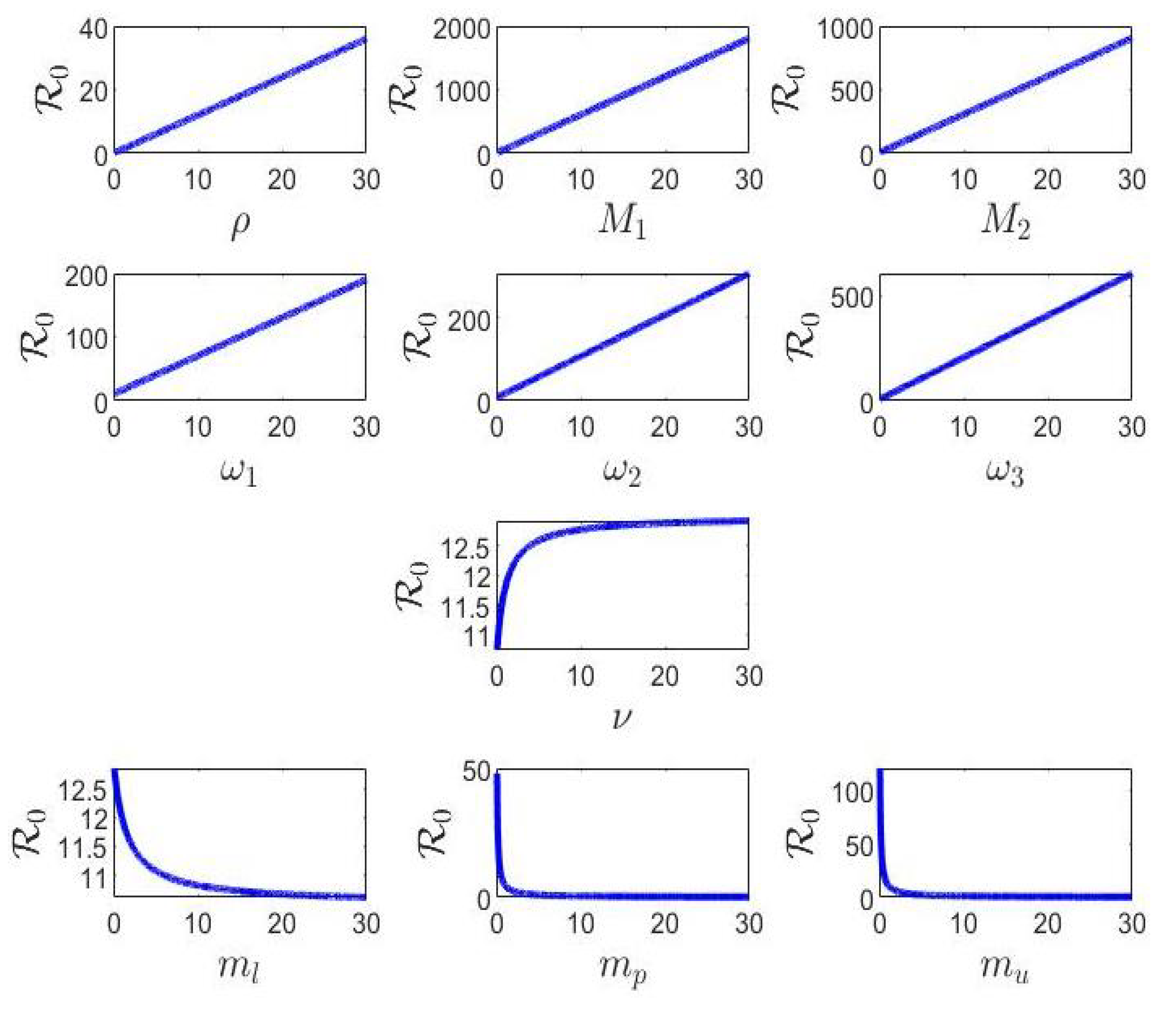
4. Sensitivity Analysis of $ℛ$₀

All diseases progress over time. This evolution is described in the disease’s mathematical modeling by variables and parameters. In this evolution, it turns out that certain parameters influence its propagation more than others. The sensitivity analysis of Model (1) was carried out in order to estimate the impact of the variation of certain parameters on the model predictions [22,23,24]. If the index describing the impact of a parameter on the model predictions is positive, then an increase of the value of the parameter induces an increase of ${\mathcal{R}}_0$, and if the index is negative, then an increase of the value of the parameter induces a decrease of ${\mathcal{R}}_0$ [24].

To find the parameters that most influence the spread of the disease, we calculated the sensitivity indices as follows.

Definition 1

(see [22,23]). The sensitivity index of ${\mathcal{R}}_0$, depending differentially on a parameter σ, is given by:

$$Y_{\sigma }^{{\mathcal{R}}_0}={\displaystyle \frac{\partial {\mathcal{R}}_0}{\partial \sigma }}\times {\displaystyle \frac{\sigma }{|{\mathcal{R}}_0|}}.$$

For instance, $Y_{\sigma }^{{\mathcal{R}}_0}=1$ implies a decrease or increase in σ, which then decreases or increases ${\mathcal{R}}_0$ accordingly. Thus, σ is the most sensitive parameter.

Proposition 1.

Recall that ${\mathcal{R}}_0$ is given by:

$$\begin{array}{c}\hfill \begin{array}{c}{\mathcal{R}}_0={\displaystyle \frac{(M_1{\omega }_2+M_2{\omega }_3)(m_l+\nu )+\nu M_1{\omega }_1}{(m_l+\nu )m_p}}{\displaystyle \frac{\varrho f^{\prime }\left(0\right)}{m_u}}.\hfill \end{array}\end{array}$$

${\mathcal{R}}_0$ depends on several parameters. The sensitivity of ${\mathcal{R}}_0$ to each one of the given parameters is given by the following sensitivity indices:

Proof. 

This follows immediately from Definition 1.    □

From

Table 2. Sensitivity of ${\mathcal{R}}_0$.

Parameter	Sensitivity Index of $ℛ$0	Sign
$\varrho$	$Y_{\varrho }^{{\mathcal{R}}_0}={\displaystyle \frac{\partial {\mathcal{R}}_0}{\partial \varrho }}\times {\displaystyle \frac{\varrho }{{\mathcal{R}}_0}}=1$	+ve
$M_1$	$Y_{M_1}^{{\mathcal{R}}_0}={\displaystyle \frac{\partial {\mathcal{R}}_0}{\partial M_1}}\times {\displaystyle \frac{M_1}{{\mathcal{R}}_0}}={\displaystyle \frac{M_1{\omega }_2(m_l+\nu )+\nu M_1{\omega }_1}{(M_1{\omega }_2+M_2{\omega }_3)(m_l+\nu )+\nu M_1{\omega }_1}}<1$	+ve
$M_2$	$Y_{M_2}^{{\mathcal{R}}_0}={\displaystyle \frac{\partial {\mathcal{R}}_0}{\partial M_2}}\times {\displaystyle \frac{M_2}{{\mathcal{R}}_0}}={\displaystyle \frac{M_2{\omega }_3(m_l+\nu )}{(M_1{\omega }_2+M_2{\omega }_3)(m_l+\nu )+\nu M_1{\omega }_1}}<1$	+ve
${\omega }_1$	$Y_{{\omega }_1}^{{\mathcal{R}}_0}={\displaystyle \frac{\partial {\mathcal{R}}_0}{\partial {\omega }_1}}\times {\displaystyle \frac{{\omega }_1}{{\mathcal{R}}_0}}={\displaystyle \frac{\nu M_1{\omega }_1}{(M_1{\omega }_2+M_2{\omega }_3)(m_l+\nu )+\nu M_1{\omega }_1}}<1$	+ve
${\omega }_2$	$Y_{{\omega }_2}^{{\mathcal{R}}_0}={\displaystyle \frac{\partial {\mathcal{R}}_0}{\partial {\omega }_2}}\times {\displaystyle \frac{{\omega }_2}{{\mathcal{R}}_0}}={\displaystyle \frac{M_1{\omega }_2(m_l+\nu )}{(M_1{\omega }_2+M_2{\omega }_3)(m_l+\nu )+\nu M_1{\omega }_1}}<1$	+ve
${\omega }_3$	$Y_{{\omega }_3}^{{\mathcal{R}}_0}={\displaystyle \frac{\partial {\mathcal{R}}_0}{\partial {\omega }_3}}\times {\displaystyle \frac{{\omega }_3}{{\mathcal{R}}_0}}={\displaystyle \frac{M_2{\omega }_3(m_l+\nu )}{(M_1{\omega }_2+M_2{\omega }_3)(m_l+\nu )+\nu M_1{\omega }_1}}<1$	+ve
$\nu$	$Y_{\nu }^{{\mathcal{R}}_0}={\displaystyle \frac{\partial {\mathcal{R}}_0}{\partial \nu }}\times {\displaystyle \frac{\nu }{{\mathcal{R}}_0}}={\displaystyle \frac{m_l{M}_1{\omega }_1\nu }{(M_1{\omega }_2+M_2{\omega }_3){(m_l+\nu )}^2+\nu M_1{\omega }_1(m_l+\nu )}}<1$	+ve
$m_l$	$Y_{m_l}^{{\mathcal{R}}_0}={\displaystyle \frac{\partial {\mathcal{R}}_0}{\partial m_l}}\times {\displaystyle \frac{m_l}{{\mathcal{R}}_0}}=-{\displaystyle \frac{m_l}{(m_l+\nu )}}{\displaystyle \frac{\nu M_1{\omega }_1}{(M_1{\omega }_2+M_2{\omega }_3)(m_l+\nu )+\nu M_1{\omega }_1}}>-1$	−ve
$m_p$	$Y_{m_p}^{{\mathcal{R}}_0}={\displaystyle \frac{\partial {\mathcal{R}}_0}{\partial m_p}}\times {\displaystyle \frac{m_p}{{\mathcal{R}}_0}}=-1$	−ve
$m_u$	$Y_{m_u}^{{\mathcal{R}}_0}={\displaystyle \frac{\partial {\mathcal{R}}_0}{\partial m_u}}\times {\displaystyle \frac{m_u}{{\mathcal{R}}_0}}=-1$	−ve

, it is clear that the parameters $\varrho ,M_1,M_2,{\omega }_1,{\omega }_2,{\omega }_3$, and $\nu$ are positive and, hence, play a vital role in controlling the stability aspects of the system. Note that the dependence of ${\mathcal{R}}_0$ on $m_l,m_p$, and $m_u$ is negative and, hence, has an adverse influence on the system.

The sensitivity analysis obtained in Table 2 can be simulated as in Figure 1 in terms of the behavior of ${\mathcal{R}}_0$ with respect to the parameters of the model. Note that ${\mathcal{R}}_0$ increases with respect to the parameters $\varrho ,M_1,M_2,{\omega }_1,{\omega }_2,{\omega }_3$, and $\nu$; however, it decreases with respect to the parameters $m_l,m_p$, and $m_u$.

5. Optimal Strategy

In this section, we propose an optimal strategy by considering a non-constant, but variable recruitment rate $\varrho \left(t\right)$ of uninfected cells to be the control function. This choice was motivated by the sensitivity analysis, since the parameter, $\varrho$, is the parameter playing the most vital role in controlling the stability aspects of the proposed model.

Assume, moreover, that f is a bounded globally Lipschitz function with ${\displaystyle \overline{f}=\underset{P>0}{sup}f\left(P\right)}$ as the upper bound and $L_f$ is the Lipschitz constant. The set of the control variables, ${\mathbf{P}}_{\mathbf{ad}}$, is given by:

$${\mathbf{P}}_{\mathbf{ad}}=\{\varrho \left(t\right):0\le {\varrho }_{min}\le \varrho \left(t\right)\le {\varrho }_{max},0\le t\le T,\varrho \left(t\right)\mathrm{is}\mathrm{Lebesgue}\mathrm{measurable}\}.$$

The goal is to look for the control variable $\varrho \left(t\right)$ and the associated state variables $U\left(t\right)$, $L\left(t\right)$, $I\left(t\right)$, $O\left(t\right)$, $P\left(t\right)$, and $C\left(t\right)$ minimizing the objective function:

$$J\left(\varrho \right)={\int }_0^T\left({\alpha }_1(L\left(t\right)+I\left(t\right)+O\left(t\right))+\frac{{\alpha }_2}{2}{\varrho }^2\left(t\right)\right)dt.$$

The choice of appropriate positive constants, ${\alpha }_1$ and ${\alpha }_2$, permits the infected population and the cost of the control to be minimized. We used the standard results [25] to prove the existence and uniqueness of both the optimal control and optimal states.

Existence and Uniqueness

For $\varphi ={\left(U,L,I,O,P,C\right)}^t$, the form of the model (1) takes a more suitable form:

$$\begin{array}{c}\hfill \begin{array}{c}{\displaystyle \dot{\varphi }=A\varphi +F\left(\varphi \right)=G\left(\varphi \right)}\hfill \end{array}\end{array}$$

(11)

where $A=\left(\begin{array}{cccccc}-m_u& 0& 0& 0& 0& 0\\ 0& -(m_l+\nu )& 0& 0& 0& 0\\ 0& \nu & -m_i& 0& 0& 0\\ 0& 0& 0& -m_o& 0& 0\\ 0& 0& M_1{m}_i& M_2{m}_o& -m_p& 0\\ 0& 0& 0& 0& \epsilon & -m_c\end{array}\right)$ and $F\left(\varphi \right)=\left(\begin{array}{c}\varrho -\omega f\left(P\right)U\\ {\omega }_{1}f\left(P\right)U\\ {\omega }_{2}f\left(P\right)U\\ {\omega }_{3}f\left(P\right)U\\ -\chi PC\\ -\upsilon PC\end{array}\right)$.

Proposition 2.

The continuous function, G, is uniformly Lipschitz.

Proof. 

The continuous function, F, is uniformly Lipschitz once:

$$\begin{array}{c}\hfill \begin{array}{ccc}\hfill \parallel F\left({\varphi }_1\right)-F\left({\varphi }_2\right){\parallel }_1& =\hfill & 2\omega |f\left(P_1\right)U_1-f\left(P_2\right)U_2|+(\chi +\upsilon )|P_1{C}_1-P_2{C}_2|\hfill \\ & =\hfill & 2\omega |f\left(P_1\right)(U_1-U_2)+(f\left(P_1\right)-f\left(P_2\right))U_2|\hfill \\ & & +(\chi +\upsilon )|P_1(C_1-C_2)+(P_1-P_2)C_2|\hfill \\ & \le \hfill & 2\omega \left(\overline{f}|U_1-U_2|+L_f|P_1-P_2|U_2\right)\hfill \\ & & +(\chi +\upsilon )\left(P_1|C_1-C_2|+C_2|P_1-P_2|\right)\hfill \\ & \le \hfill & 2\omega \left(\overline{f}|U_1-U_2|+L_f{\displaystyle \frac{\varrho }{m_1}}|P_1-P_2|\right)\hfill \\ & & +(\chi +\upsilon ){\displaystyle \frac{\varrho (m_i{M}_1+m_o{M}_2)}{m_1{m}_2}}|C_1-C_2|\hfill \\ & & +(\chi +\upsilon ){\displaystyle \frac{2\epsilon }{m_p}}{\displaystyle \frac{\varrho (m_i{M}_1+m_o{M}_2)}{m_1{m}_2}}|P_1-P_2|\hfill \\ & \le \hfill & 2\overline{f}\omega |U_1-U_2|+(\chi +\upsilon ){\displaystyle \frac{\varrho (m_i{M}_1+m_o{M}_2)}{m_1{m}_2}}|C_1-C_2|\hfill \\ & & +\left[2L_f{\displaystyle \frac{\varrho }{m_1}}\omega +(\chi +\upsilon ){\displaystyle \frac{2\epsilon }{m_p}}{\displaystyle \frac{\varrho (m_i{M}_1+m_o{M}_2)}{m_1{m}_2}}\right]|P_1-P_2|\hfill \\ & \le \hfill & {\displaystyle M_F\parallel {\varphi }_1-{\varphi }_2{\parallel }_1}\hfill \end{array}\end{array}$$

where:

$$M_F=max\left(2\overline{f}\omega ,(\chi +\upsilon ){\displaystyle \frac{\varrho (m_i{M}_1+m_o{M}_2)}{m_1{m}_2}},\left[2L_f{\displaystyle \frac{\varrho }{m_1}}\omega (\chi +\upsilon ){\displaystyle \frac{2\epsilon }{m_p}}{\displaystyle \frac{\varrho (m_i{M}_1+m_o{M}_2)}{m_1{m}_2}}\right]\right).$$

Since,

$$\begin{array}{c}\hfill \begin{array}{c}\hfill {\displaystyle \parallel A{\varphi }_1-A{\varphi }_2{\parallel }_1\le \parallel A{\parallel }_1\parallel {\varphi }_1-{\varphi }_2{\parallel }_1}\end{array}\end{array}$$

(12)

where $\parallel A{\parallel }_1:={sup}_{X\ne 0}\frac{\parallel AX{\parallel }_1}{\parallel X{\parallel }_1}$ is the matrix norm of A where $\parallel ·{\parallel }_1$ is the vector norm. Therefore,

$$\begin{array}{c}\hfill \begin{array}{c}\hfill {\displaystyle \parallel G\left({\varphi }_1\right)-G\left({\varphi }_2\right){\parallel }_1\le M_G\parallel {\varphi }_1-{\varphi }_2{\parallel }_1}\end{array}\end{array}$$

(13)

here $M_G=max(M_F,\parallel A\parallel )$. It is easy, now, to deduce that the continuous function, G, is uniformly Lipschitz.    □

Since the function, G, is a uniformly Lipschitz continuous function, then System (11) admits a unique solution.

Pontryagin’s maximum principle [25,26,27] permits the derivation of some necessary conditions to calculate the optimal control and states. The expression of the Hamiltonian is given by:

$$\begin{array}{c}\hfill \begin{array}{ccc}H\hfill & =\hfill & {\alpha }_1(L+I+O)+{\displaystyle \frac{{\alpha }_2}{2}}{\varrho }^2+{\lambda }_1\dot{U}+{\lambda }_2\dot{L}+{\lambda }_3\dot{I}+{\lambda }_4\dot{O}+{\lambda }_5\dot{P}+{\lambda }_6\dot{C}\hfill \\ & =\hfill & {\alpha }_1(L+I+O)+{\displaystyle \frac{{\alpha }_2}{2}}{\varrho }^2+{\lambda }_1(\varrho -\omega f\left(P\right)U-m_{u}U)\hfill \\ & & +{\lambda }_2({\omega }_{1}f\left(P\right)U-(m_l+\nu )L)+{\lambda }_3({\omega }_{2}f\left(P\right)U+\nu L-m_{i}I)\hfill \\ & & +{\lambda }_4({\omega }_{3}f\left(P\right)U-m_{o}O)+{\lambda }_5(M_1{m}_{i}I+M_2{m}_{o}O-m_{p}P-\chi PC)\hfill \\ & & +{\lambda }_6(\epsilon P-m_{c}C-\upsilon PC).\hfill \end{array}\end{array}$$

(14)

For a given optimal control, ${\varrho }^{*}$, we derive the adjoint states ${\lambda }_1,{\lambda }_2,{\lambda }_3,{\lambda }_4,{\lambda }_5$, and ${\lambda }_6$ related to the states $U,L,I,O,P$, and C as the following:

$$\left\{\begin{array}{ccc}{\dot{\lambda }}_1=-{\displaystyle \frac{\partial H}{\partial U}}\hfill & =\hfill & {\lambda }_1(\omega f\left(P\right)+m_u)-{\omega }_1{\lambda }_{2}f\left(P\right)-{\omega }_2{\lambda }_{3}f\left(P\right)-{\omega }_3{\lambda }_{4}f\left(P\right),\hfill \\ {\dot{\lambda }}_2=-{\displaystyle \frac{\partial H}{\partial L}}\hfill & =\hfill & -{\alpha }_1+{\lambda }_2(m_l+\nu )-{\lambda }_3\nu ,\hfill \\ {\dot{\lambda }}_3=-{\displaystyle \frac{\partial H}{\partial I}}\hfill & =\hfill & -{\alpha }_1+m_i{\lambda }_3-m_i{M}_1{\lambda }_5,\hfill \\ {\dot{\lambda }}_4=-{\displaystyle \frac{\partial H}{\partial O}}\hfill & =\hfill & -{\alpha }_1+m_o{\lambda }_4-m_o{M}_2{\lambda }_5,\hfill \\ {\dot{\lambda }}_5=-{\displaystyle \frac{\partial H}{\partial P}}\hfill & =\hfill & {\lambda }_1\omega f^{\prime }\left(P\right)U-{\lambda }_2{\omega }_1{f}^{\prime }\left(P\right)U-{\lambda }_3{\omega }_2{f}^{\prime }\left(P\right)U-{\lambda }_4{\omega }_3{f}^{\prime }\left(P\right)U\hfill \\ & & +{\lambda }_5(m_p+\chi C)-{\lambda }_6(\epsilon -\upsilon C),\hfill \\ {\dot{\lambda }}_6=-{\displaystyle \frac{\partial H}{\partial C}}& =& {\lambda }_6(m_c+\upsilon P)+\chi {\lambda }_{5}P.\hfill \end{array}\right.$$

where ${\lambda }_i\left(T\right)=0$ with $i=1,\cdots ,6$ are the final conditions.

The slope of the Hamiltonian is given by:

$${\displaystyle \frac{\partial H}{\partial \varrho }}={\alpha }_2\varrho +{\lambda }_1.$$

(15)

The root of the equation ${\displaystyle \frac{\partial H}{\partial \varrho }}=0$ for anon-trivial interval of time has to be between its upper and lower bounds. Thus, the control expression is given by:

$$\varrho \left(t\right)=-\frac{{\lambda }_1}{{\alpha }_2}\mathrm{if}{\alpha }_2\ne 0\mathrm{and}{\varrho }_{min}\le -\frac{{\lambda }_1}{{\alpha }_2}\le {\varrho }_{max}.$$

Thus, the control characterization is:

$$\begin{array}{c}\mathrm{If}{\displaystyle \frac{\partial H}{\partial \varrho }}<0\mathrm{at}t,\mathrm{then}{\varrho }^{*}\left(t\right)={\varrho }_{max};\\ \mathrm{If}{\displaystyle \frac{\partial H}{\partial \varrho }}>0\mathrm{at}t,\mathrm{then}{\varrho }^{*}\left(t\right)={\varrho }_{min};\\ \mathrm{If}{\displaystyle \frac{\partial H}{\partial \varrho }}=0,\mathrm{then}\varrho \left(t\right)=-\frac{{\lambda }_1}{{\alpha }_2};\end{array}$$

such that ${\alpha }_2\ne 0$ and ${\varrho }_{min}\le -{\displaystyle \frac{{\lambda }_1}{{\alpha }_2}}\le {\varrho }_{max}$.

6. Numerical Results and Conclusions

For the numerical simulations, we considered a nonlinear incidence rate of the form $f\left(P\right)={\displaystyle \frac{\overline{f}}{k+P}}$ named the Monod function (also Holling’s type II). This form of function has been widely used to describe the transmission rate of diseases. $\overline{f}$ and k are two constants. Note that the continuous function f is globally Lipschitz with a Lipschitz constant $\overline{f}/k$. The parameter values given in

Table 3. Parameters’ values used for the numerical investigations.

Parameter	${\mathit{\omega }}_1$	${\mathit{\omega }}_2$	${\mathit{\omega }}_3$	${\mathit{m}}_{\mathit{u}}$	${\mathit{m}}_{\mathit{l}}$	${\mathit{m}}_{\mathit{i}}$	${\mathit{m}}_{\mathit{o}}$	${\mathit{m}}_{\mathit{p}}$	${\mathit{m}}_{\mathit{c}}$
Value	$0.25$	$0.45$	$0.3$	1	1	$3.4$	$2.4$	$0.4$	$1.4$
Parameter	$\mathit{\nu }$	${\mathit{M}}_1$	${\mathit{M}}_2$	$\mathit{ϵ}$	$\mathit{\chi }$	$\mathit{\upsilon }$	$\overline{\mathit{f}}$	k
Value	$1.5$	$0.1$	$0.2$	$2.5$	$0.9$	$0.2$	8	2

were used for all numerical investigations presented in this section.

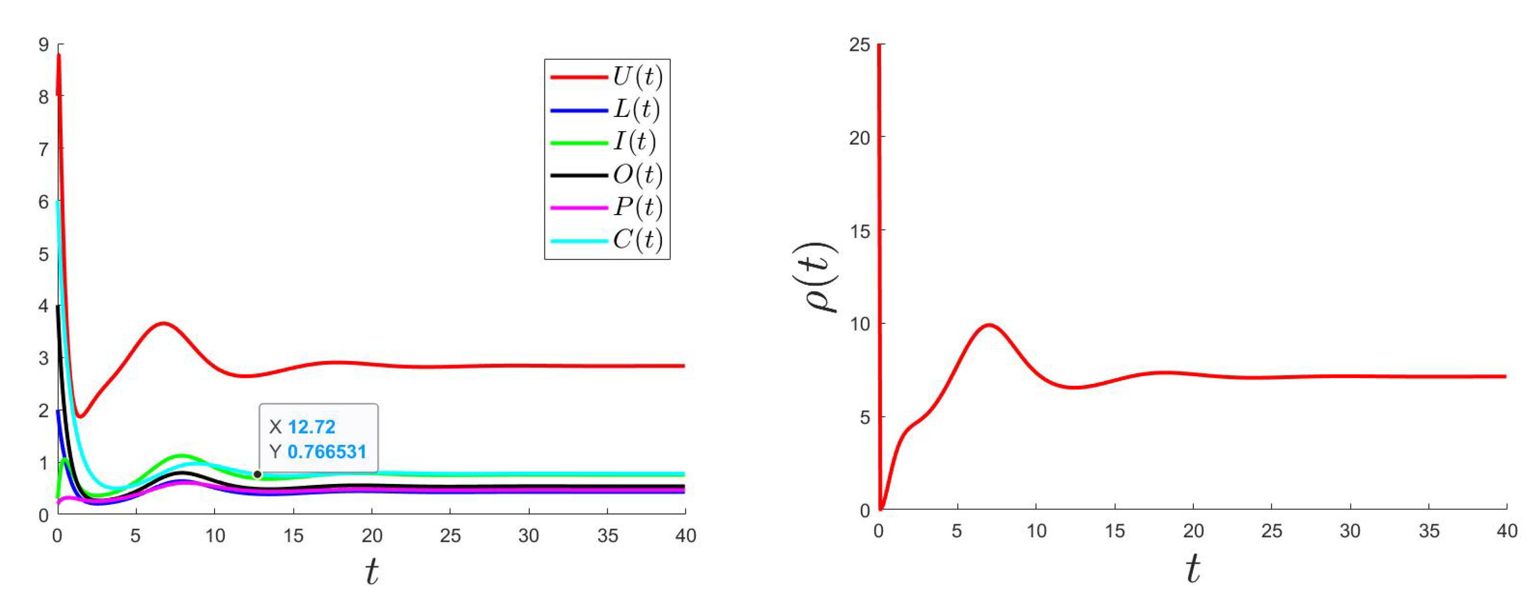
6.1. Direct Problem

For $\varrho =10$, then ${\mathcal{R}}_0=10>1$, the trajectory of the model (1) converges to $E^{*}$ (Figure 2).

Similarly, for $\varrho =2$, then ${\mathcal{R}}_0=2>1$, the trajectory of the model (1) converges to $E^{*}$ (Figure 3). Thus, the global stability of the equilibrium point $E^{*}$ is when ${\mathcal{R}}_0>1$. This confirms the findings of Theorem 2.

For $\varrho =0.8$, then ${\mathcal{R}}_0=0.8<1$, the trajectory of the model (1) converges to $E_0=(0.8,0,0,0,0,0)$ (Figure 4). Thus, the global stability of the equilibrium point $E_0=({\displaystyle \frac{\varrho }{m_u}},0,0,0,0,0)$ is when ${\mathcal{R}}_0\le 1$. This confirms the findings of Theorem 1.

6.2. Control Problem

The control problem was resolved using an improved Gauss–Seidel-like implicit numerical scheme (for more details, please see Appendix C). We used the same parameter values as the ones used for Figure 2 (where $E^{*}$ is GAS) considering a variable $\varrho$ such that $\varrho \left(0\right)=25$ and with the bounds ${\varrho }^{min}=0$ and ${\varrho }^{max}=50$.

Figure 5, Figure 6 and Figure 7 show the plotted behaviors of $\varrho$ (right), $U\left(t\right),L\left(t\right),I\left(t\right),O\left(t\right),P\left(t\right)$, and $C\left(t\right)$ (left) for different values of ${\alpha }_1$ and ${\alpha }_2$.

7. Conclusions

The human immunodeficiency virus (HIV) is the pathogen responsible for acquired immunodeficiency syndrome (AIDS). Mathematical modeling enables public health workers to compare, plan, execute, evaluate, and optimize different programs for detection, prevention, therapy, and control. This also helps identify trends and make general forecasts.

In this paper, we considered a mathematical 6D dynamic model for HIV transmission with a general incidence rate. The analysis of the local and global stability of the equilibrium points permitted us to conclude that the infected steady state ($E^{*}$) is globally asymptotically stable once ${\mathcal{R}}_0>1$ and the disease-free steady state ($E_0$) is globally asymptotically stable once ${\mathcal{R}}_0\le 1$. The sensitivity analysis was carried out for the proposed model. Based on this analysis, an optimal strategy was formulated where the goal was to minimize the number of infected cells. The theoretical findings were validated by some numerical results.

References

- Douek, C.D.; Mario, R.; Koup, R.A. Emerging Concepts in the Immunopathogenesis of AIDS. Annu. Rev. Med. 2009, 60, 471–484. [Google Scholar] [CrossRef] [PubMed] [Green Version]
- Bernoulli, D. Essai d’une nouvelle analyse de la mortalité causée par la petite vérole et des avantages de l’inoculation pour la prévenir. Mem. Math. Phys. Acad. Roy. Sci. Paris 1760, 1–45. [Google Scholar]
- Diekmann, O.; Heesterbeek, J. On the definition and the computation of the basic reproduction ratio R0 in models for infectious diseases in heterogeneous populations. J. Math. Biol. 1990, 28, 365–382. [Google Scholar] [CrossRef] [PubMed] [Green Version]
- Hethcote, H. The mathematics of infectious disease. SIAM Rev. 2000, 42, 599–653. [Google Scholar] [CrossRef] [Green Version]
- Gumel, A.; Shivakumar, P.; Sahai, B. A mathematical model for the dynamics of HIV-1 during the typical course of infection. Nonlinear Anal. Theory Methods Appl. Ser. A Theory Methods 2001, 47, 1773–1783. [Google Scholar] [CrossRef]
- Alshehri, A.; El Hajji, M. Mathematical study for Zika virus transmission with general incidence rate. AIMS Math. 2022, 7, 7117–7142. [Google Scholar] [CrossRef]
- El Hajji, M.; Albargi, A.H. A mathematical investigation of an “SVEIR” epidemic model for the measles transmission. Math. Biosci. Eng. 2022, 19, 2853–2875. [Google Scholar] [CrossRef]
- El Hajji, M.; Sayari, S.; Zaghdani, A. Mathematical analysis of an SIR epidemic model in a continuous reactor—Deterministic and probabilistic approaches. J. Korean Math. Soc. 2021, 58, 45–67. [Google Scholar] [CrossRef]
- Asamoah, J.K.K.; Okyere, E.; Abidemi, A.; Moore, S.E.; Sun, G.Q.; Jin, Z.; Acheampong, E.; Gordon, J.F. Optimal control and comprehensive cost-effectiveness analysis for COVID-19. Results Phys. 2022, 33, 105177. [Google Scholar] [CrossRef]
- Elaiw, A.; AlShehaiween, S.; Hobiny, A. Global properties of HIV dynamics models including impairment of B-cell functions. J. Biol. Syst. 2020, 28, 1–25. [Google Scholar] [CrossRef]
- Perelson, A.S.; Neumann, A.U.; Markowitz, M.; Leonard, J.M.; Ho, D.D. HIV-1 dynamics in vivo: Virion clearance rate, infected cell life-span, and viral generation time. Science 1996, 271, 1582–1586. [Google Scholar] [CrossRef] [Green Version]
- den Driessche, P.V.; Watmough, J. Reproduction Numbers and Sub-Threshold Endemic Equilibria for Compartmental Models of Disease Transmission. Math. Biosci. 2002, 180, 29–48. [Google Scholar] [CrossRef]
- LaSalle, J. The Stability of Dynamical Systems; SIAM: Philadelphiam, PA, USA, 1976. [Google Scholar]
- Alsahafi, S.; Woodcock, S. Local Analysis for a Mutual Inhibition in Presence of Two Viruses in a Chemostat. Nonlinear Dyn. Syst. Theory 2021, 21, 337–359. [Google Scholar]
- Alsahafi, S.; Woodcock, S. Mathematical Study for Chikungunya Virus with Nonlinear General Incidence Rate. Mathematics 2021, 9, 2186. [Google Scholar] [CrossRef]
- Alsahafi, S.; Woodcock, S. Mutual inhibition in presence of a virus in continuous culture. Math. Biosc. Eng. 2021, 18, 3258–3273. [Google Scholar] [CrossRef]
- El Hajji, M. How can inter-specific interferences explain coexistence or confirm the competitive exclusion principle in a chemostat. Int. J. Biomath. 2018, 11, 1850111. [Google Scholar] [CrossRef]
- El Hajji, M. Modelling and optimal control for Chikungunya disease. Theory Biosci. 2021, 140, 27–44. [Google Scholar] [CrossRef] [PubMed]
- El Hajji, M.; Zaghdani, A.; Sayari, S. Mathematical analysis and optimal control for Chikungunya virus with two routes of infection with nonlinear incidence rate. Int. J. Biomath. 2022, 15, 2150088. [Google Scholar] [CrossRef]
- El Hajji, M.; Chorfi, N.; Jleli, M. Mathematical model for a membrane bioreactor process. Electron. J. Diff. Eqns. 2015, 2015, 1–7. [Google Scholar]
- El Hajji, M.; Chorfi, N.; Jleli, M. Mathematical modelling and analysis for a three-tiered microbial food web in a chemostat. Electron. J. Diff. Eqns. 2017, 2017, 1–13. [Google Scholar]
- Chitnis, N.; Hyman, J.; Cushing, J. Determining important parameters in the spread of malaria through the sensitivity analysis of a mathematical model. Bull. Math. Biol. 2008, 70, 1272–1296. [Google Scholar] [CrossRef] [PubMed]
- Silva, C.; Torres, D. Optimal control for a tuberculosis model with reinfection and post-exposure interventions. Math. Biosci. 2013, 244, 154–164. [Google Scholar] [CrossRef] [PubMed] [Green Version]
- Rodrigues, H.; Teresa, M.; Monteiro, T.; Torres, D. Sensitivity Analysis in a Dengue Epidemiological Model. In Hindawi Publishing Corporation Conference Papers in Mathematics; Hindawi: London, UK, 2013; p. 721406. [Google Scholar]
- Fleming, W.; Rishel, R. Deterministic and Stochastic Optimal Control; Springer: New York, NY, USA, 1975. [Google Scholar]
- Lenhart, S.; Workman, J. Optimal Control Applied to Biological Models; Chapman and Hall: London, UK, 2007. [Google Scholar]
- Pontryagin, L.; Boltyanskii, V.; Gamkrelidze, R.V.; Mishchenko, E.F. The Mathematical Theory of Optimal Processes; Wiley: New York, NY, USA, 1962. [Google Scholar]
- Hurwitz, A. “Ueber die Bedingungen, unter welchen eine Gleichung nur Wurzeln mit negativen reellen Theilen besitzt”. (English translation “On the conditions under which an equation has only roots with negative real parts” by H. G. Bergmann in Selected Papers on Mathematical Trends in Control Theory R. Bellman and R. Kalaba Eds. New York: Dover, 1964 pp. 70–82.). Math. Ann. 1895, 46, 273–284. [Google Scholar] [CrossRef]
- Routh, E.J. A Treatise on the Stability of a Given State of Motion: Particularly Steady Motion; Macmillan and Company: New York, NY, USA, 1877. [Google Scholar]
Figure 1.
Behavior of .
Figure 2.
Behaviors for and then .
Figure 3.
Figure 4.