Article

Abnormality Detection and Failure Prediction Using Explainable Bayesian Deep Learning: Methodology and Case Study with Industrial Data

by
Ahmad Kamal Mohd Nor
1,*,
Srinivasa Rao Pedapati
1,
Masdi Muhammad
1 and
Víctor Leiva
2
1
Mechanical Department, Universiti Teknologi Petronas, Seri Iskandar 32610, Malaysia
2
School of Industrial Engineering, Pontificia Universidad Católica de Valparaíso, Valparaíso 2362807, Chile
*
Author to whom correspondence should be addressed.
Mathematics 2022, 10(4), 554; https://doi.org/10.3390/math10040554
Submission received: 11 January 2022 / Revised: 3 February 2022 / Accepted: 8 February 2022 / Published: 11 February 2022

Abstract

:
Mistrust, amplified by numerous artificial intelligence (AI) related incidents, is an issue that has caused the energy and industrial sectors to be amongst the slowest adopter of AI methods. Central to this issue is the black-box problem of AI, which impedes investments and is fast becoming a legal hazard for users. Explainable AI (XAI) is a recent paradigm to tackle such an issue. Being the backbone of the industry, the prognostic and health management (PHM) domain has recently been introduced into XAI. However, many deficiencies, particularly the lack of explanation assessment methods and uncertainty quantification, plague this young domain. In the present paper, we elaborate a framework on explainable anomaly detection and failure prognostic employing a Bayesian deep learning model and Shapley additive explanations (SHAP) to generate local and global explanations from the PHM tasks. An uncertainty measure of the Bayesian model is utilized as a marker for anomalies and expands the prognostic explanation scope to include the model’s confidence. In addition, the global explanation is used to improve prognostic performance, an aspect neglected from the handful of studies on PHM-XAI. The quality of the explanation is examined employing local accuracy and consistency properties. The elaborated framework is tested on real-world gas turbine anomalies and synthetic turbofan failure prediction data. Seven out of eight of the tested anomalies were successfully identified. Additionally, the prognostic outcome showed a 19% improvement in statistical terms and achieved the highest prognostic score amongst best published results on the topic.

1. Introduction

1.1. Artificial Intelligence

Artificial intelligence (AI) is officially the hype of the century, unraveling possibilities that once resided only in our imagination. AI is currently serving numerous fields and constantly breaking fresh boundaries. Its capability is consumed by the mass public and reaches far into specialized domains. The intensive race between world powers to harness its power stimulates a consistent stream of funds to support AI-based projects in all parts of the globe. With AI technology presently within reach by literally everyone, the age of AI has just begun.
How does one define AI? According to a survey conducted by Artificial General Intelligence Sentinel Initiative in 2018, the most agreeable definition for AI voted by experts is that stated in [1]. There, AI is described as having the faculty of adaptation and improvisation, despite possessing limited knowledge and resources. The description further implies the autonomy and learning capacity of the system.
The European Commission describes AI as similar to the former definition, but without the concept of limitation, albeit carefully specifying the system’s partial degree of autonomy [2]. These depictions paint us the picture of a system capable of reasoning and operating with partial or no supervision at all, thus potentially beneficial or dangerous to the human being. The type and task of AI methods are commonly classified into seven categories, as follows:
(i)
Machine learning: This is based on deep learning and predictive analytics.
(ii)
Natural language processing: This is related to translation, classification, and information extraction.
(iii)
Speech: This is visualized as speech to text and text to speech.
(iv)
Expert systems: This corresponds to inference engine and knowledge base.
(v)
Planning, schedule, optimization: This is associated with reduction (transforming complex planning challenges into other forms such as the Boolean satisfiability problem), classical (completely deterministic planning with one initial state), probabilistic (planning under uncertainty and incomplete information), as well as temporal (planning by the incorporation of duration and concurrency of actions and events).
(vi)
Robotic: This considers reactive machine, limited memory, theory of mind, and self-aware.
(vii)
Vision: This is based on image recognition and computer/machine vision.
Such a vast catalog of abilities naturally finds its worth in many applications. Globally, the impact of AI is more anticipated in crucial economic and social pillars, such as manufacturing, transportation, healthcare, business analytics, finance, and retail [3,4]. Likewise, research on AI stretches over other niche domains such as entertainment [5], law enforcement [6], security [7], safety [8], defense [9], construction [10], investment [11], and mining operations [12]. The list goes on with endless possibilities, with new fronts being opened by researchers daily.
Machine learning and deep learning have emerged as the most popular and powerful tools in solving technical challenges [13,14,15,16]. Their nonlinearity power, ever-increasing data volume, availability of open-source development tools within reach by everyone, together with enhanced and affordable computing power, push deep learning to the forefront of AI tools. Some of the notable deep learning achievements throughout the decade are mentioned here. In the speech recognition field, deep learning outperformed the Gaussian mixture modeling-based systems with record accuracy [17]. Alpha Go, an AI game system, beat world champions, Lee Sedol and Ke Jie, in the Go game match in 2016 and 2017, respectively [18,19]. In robotics, the OpenAI Five robot system beat the world champion team in 2019 in the Dota game tournament [18]. In 2021, CoAtNet-7 achieved 90.88% accuracy in ImageNet image classification dataset [20].
The AI investment landscape is diversified and dynamic. Price Water Cooper estimated that AI could uplift global GDP by 14% or $15.7 trillion by 2030, with China and the United States (US) as the biggest beneficiaries of this impact [21]. In 2019, the US possessed the most investment under the form of private AI companies, representing around 64% of the global share, followed by China. The rest of the world trails the US and China, contracting around 400% in investment value from 2015 to 2019. During the said epoque, transportation, customer relations, and business analytics received the biggest specific investments in the US while transportation, security, and arts attracted more investment in China. Globally, transportation and business analytic sectors constitute important investment grounds [22]. Soon, AI will fully replace capital and labor as the new factors of production, being the main driver of productivity [21]. The labor market will experience profound change where less workforce generating higher value will be required. To thrive or merely survive the competition, increasing AI assimilation to replace low-skilled works is expected to be the future agenda in the industries [23].
According to the World Intellectual Property Organization, the number of new AI patents registered tripled from 2013 to 2017, mirroring the intensive efforts led by the technical community in exploiting AI potential to overcome challenges [24]. Geographically, the top world economies, majorly in Asia, occupy the biggest share in AI patent registration headed by Japan (43%), followed by the US (20%), European Union (10%), China (10%), South Korea (10%), and Germany (3%). The primary sectors where patent and trademark registrations are concentrated correspond to computers and electronics, machinery, information technology services, and transportation [25].
Surprisingly, the industrial, manufacturing, and energy sectors are amongst the slowest to adopt AI in their day-to-day operations [21]. Considering the continuous improvement ethic in these areas, such slowness seems to be improbable. However, one can understand that there is a confidence issue from the industrial actors to blindly accept AI decisions. Thus, trust is the primary obstacle in AI implementation. In the industrial sectors, this mistrust is more related to performance issues. In other areas, different types of problems might arise. The Center for Security and Emerging Technology defines the category of AI malfunction as follows [26]:
(i)
Failures of robustness: The system is subjected to unusual or unforeseen inputs, causing failures.
(ii)
Failures of specification: The system is attempting to do something that is subtly different from what the developer anticipated, which might result in surprising behaviors or consequences.
(iii)
Failures of assurance: In operational mode, the system cannot be fully supervised or regulated.
The AI incident database (www.incidentdatabase.ai, accessed on 3 December 2021) documents the growing AI incidents since 2019 [27]. This repertoire exhibits several pieces of information worth noting. Today, the top domains where incidents are reported are transportation, healthcare, manufacturing, and nuclear, as presented in Figure 1a. Most of the incidents are caused by machine learning issues as shown in Figure 1b. These facts strengthen the belief about why the industrial and energy sectors are hesitant in using AI. On a more serious note, 8% of the incidents resulted in the loss of lives.
The emerging AI laws is another challenge. The rise of incidents and their consequences risk to stall investments and prompted the call for regulations. The laws intend not to punish but to foster a responsible AI culture. A summary of global AI regulations can be found in [28]. Included is the General Data Protection Regulation, which is the strictest regulation to date issued by Europe. This regulation would affect developers around the world whose system’s output is related to Europe. Such a regulation classifies AI systems into three categories as (a) limited and minimal risk, (b) high risk, and (c) unacceptable risk. The unacceptable-risk system will not be authorized anymore while the high-risk system will be conditioned to strict requirements. The minimal-risk system will also be subject to a few conditions. Under this law, offenses could incur fines of up to € 30 million or 6% of global revenue with the use of illegal systems, and the breach of the data-governance requirements, by employing hazardous systems, could result in the heftiest penalties.
In brief, there are six system’s qualities demanded towards a responsible AI framework, stated as:
(i)
Transparency: An AI system mechanism should be understood.
(ii)
Reliability and safety: An AI system should work as intended and be safe to use.
(iii)
Privacy and security: AI systems should respect confidentiality and be protected.
(iv)
Fairness: AI systems should behave equally toward all human beings.
(v)
Inclusiveness: AI systems should inspire and promote human participation.
(vi)
Accountability: Responsibility measures must be available when the AI system malfunctions.
Note that most of the provisions in the law focus on the issue of transparency, fairness, privacy, and data security related to AI algorithms. Transparency refers to the mechanism of AI methods in obtaining their output. In fact, transparency is the main key in minimizing AI malfunctions and achieving the AI quality goals mentioned before. This aspect is vital due to the black-box characteristic of some AI techniques.
Deep learning, being the most powerful AI method until now, is a black-box model so that it is opaque. Though very effective, its mechanism in generating forecasts is unknown. Naturally, this opacity thwarts AI dissemination in high-stakes areas, such as the industry and energy sectors, where the incomprehensible outcome could lead to incorrect predictions. In turn, this can provoke disastrous effects in terms of life, safety, and finances. Obviously, the experts of each area demand more than mere point estimate prediction to convince them to take the correct course of action. Thus, the ball lies in the research community’s hands to diminish this mistrust. This is where explainable AI (XAI) enters the scene.
The XAI is a field dedicated to making AI models transparent to humans through various approaches. Though this notion has been known for decades, global attention garnered in XAI shows a notable rise more recently, reflected by the increasing initiatives by various parties, including the Defense Advanced Research Projects Agency since 2016 [29]. The steady accumulation in general and specialized review articles on XAI translates to the growing interest in XAI from the research community [30,31,32,33,34]. This sudden spike in interest on XAI is partly due to emerging laws as mentioned previously. However, the advantages of XAI far outweigh the need for regulations based on:
(i)
Justifying the model’s decision, detecting its problems, especially during the trial period of the AI model, strengthening reliability and safety.
(ii)
Complying with the regulations, transparency that leads to accountability, enhanced security, and data privacy.
(iii)
Helping to understand AI reasoning and decrease problems related to fairness in AI use.
(iv)
Assisting practitioners in verifying the required proprieties of the AI system from the developer.
(v)
Promoting interactivity and expanding human creativity by discovering new perspectives on the model or the data.
(vi)
Allowing resources to be more optimized, avoiding wastage.
(vii)
Fostering collaboration between experts, data scientists, users, and stakeholders.
Several published articles have organized XAI approaches into distinct taxonomies [35,36,37]. This paper briefly describes the categorization according to [35], which falls into two general categories. Firstly, we consider transparent models, which are directly interpretable due to their simple structure or comprehensible visualization such as linear or logistic regression, decision tree, and rule-based methods. Secondly, we consider post-hoc explainability, where the explanation is generated after the model to be explained is trained. Included in this category is the model agnostic approach, an external method that can be used with any AI model. In addition, post-hoc explainability is applied for shallow machine learning models (tree ensembles, random forests, multiple classifier systems, and support vector machines). Then, the approaches related to deep learning are considered, such as neural networks (model simplification and feature relevance), techniques appropriate only for certain deep learning models such as convolutional neural network and recurrent neural network, layer-wise relevance propagation, class activation mapping, gradient weighted class activation mapping, and hybrid-transparent-opaque models such as knowledge-based and case-based reasoning.
As the backbone of the industry, prognostic and health management (PHM) is a set of frameworks exploiting sensor signals to safeguard the health state of industrial assets by identifying, examining, and tracking degradation and estimating failure evolution [38]. To achieve this goal, three main activities, comprising of anomaly detection, failure prognostic, and diagnostic, are employed:
(i)
The first activity consists of identifying outliers in the system’s output data [39,40].
(ii)
The second activity englobes the determination of remaining useful life (RUL) [41].
(iii)
Lastly, we have the activity of classification and identification of the root cause of failure [42].
In recent years, AI has become a predominant tool in reliability-based research [43]. PHM-XAI is still a very young discipline as testified by the recent systematic review on PHM-XAI presented in [44] and shown in Figure 2a, where several peer-reviewed journal articles treating the subject demonstrate that the PHM-XAI is still scarcely studied but steadily rising. Several explainability approaches have been explored by the PHM-XAI researchers. To forge trust in AI and facilitate its legal use in the industry, it is urgent to disseminate the XAI know-how to the PHM players, in both the research and industrial domains.

1.2. Research Gaps and Opportunities

The review presented in [44] further lists several deficiencies plaguing the research in PHM-XAI that need to be remedied promptly, considering:
(i)
Lack of human involvement: Human engagement is crucial for assessing the generated explanation as the latter is meant for them. Furthermore, human–AI cooperation could contribute to the integration of human-related sciences and for the development of interactive AI, where experts and AI systems work hand in hand, providing more assurance in the AI system’s output.
(ii)
Explanation evaluation is practically absent: These measures are important for researchers and developers when evaluating explanation quality.
(iii)
Insufficiency in uncertainty management: Uncertainty quantification safeguards the system against adversarial examples where false explanations could be generated from unseen, new data. Moreover, it provides users with supplementary confidence in trusting AI methods prediction compared to point estimation statistical models. It is thus inconceivable for a working AI system to be devoid of this feature.
A summary of research opportunities in PHM-XAI was provided in [44], indicating that:
(i)
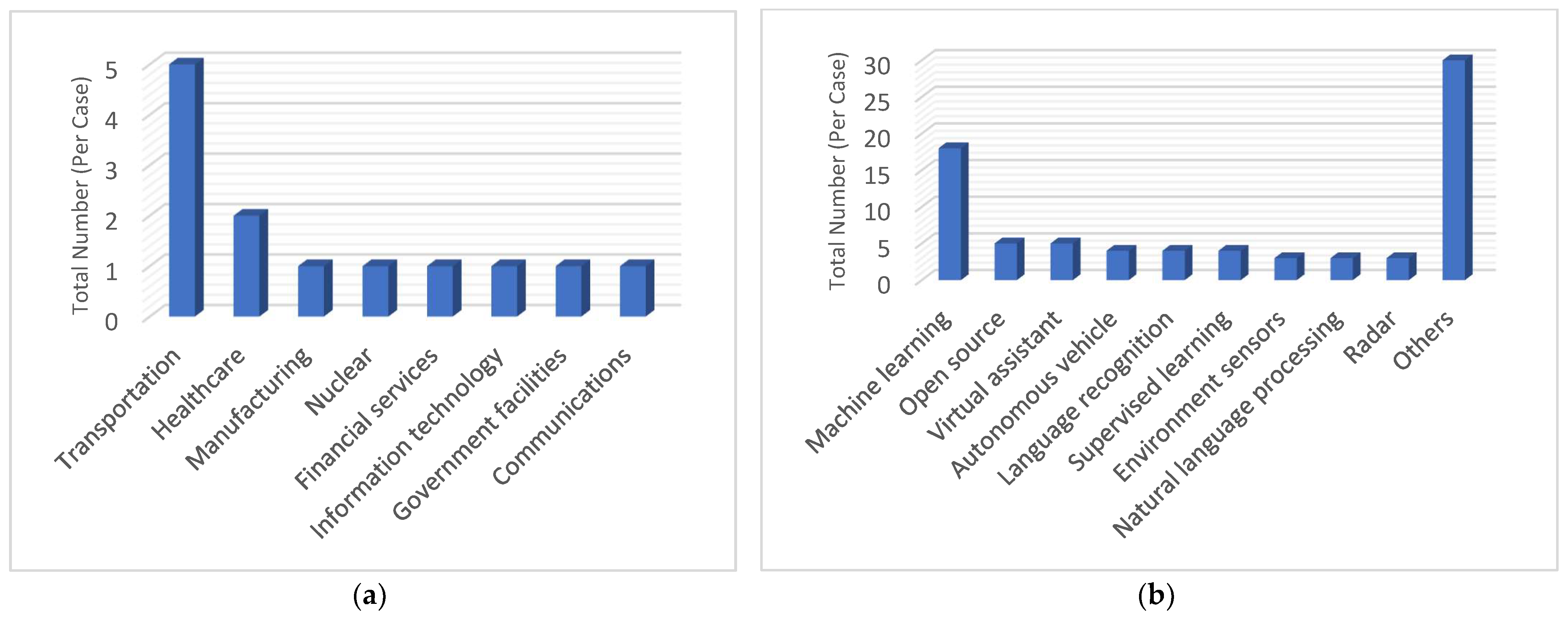
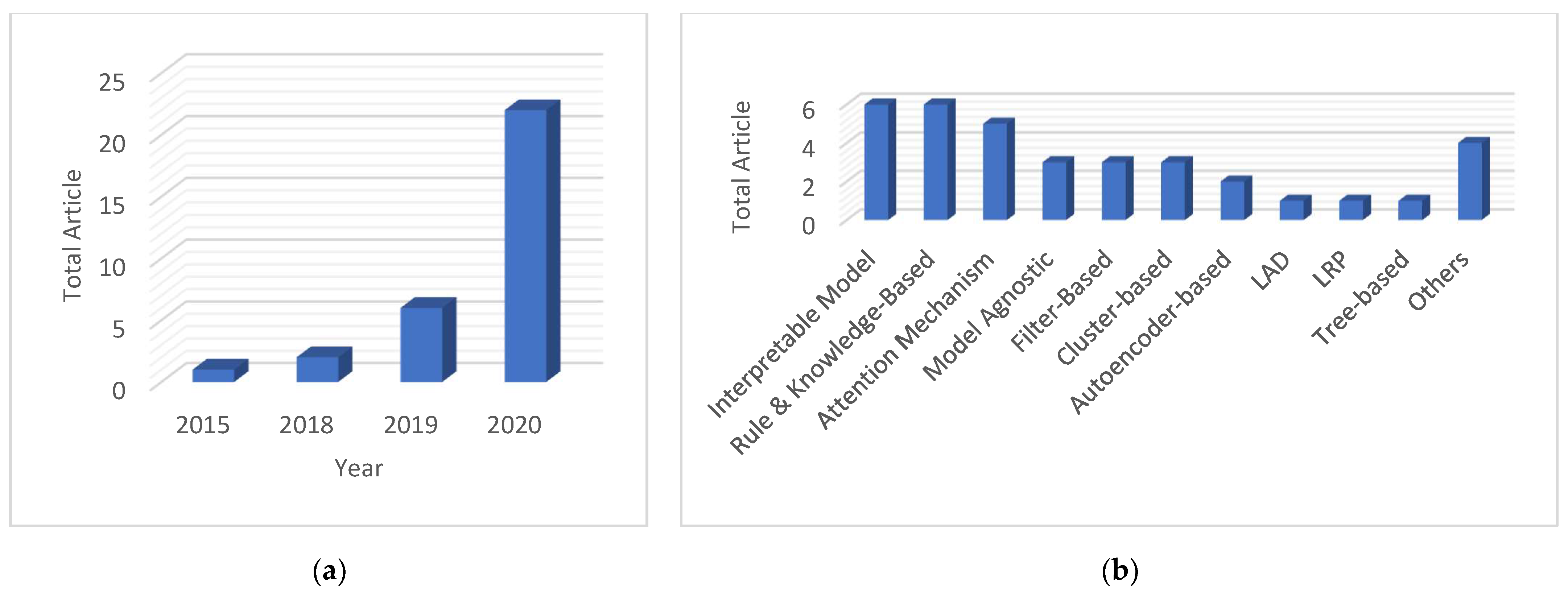
As shown in Figure 2b, model agnostic explainability, layer-wise relevance propagation, and logic analysis of data are less explored, but they possess great potential as they could be used with any black-box model without altering its performance.
(ii)
While Shapley additive explanations (SHAP) is an established method and employed in previous works, note that it was not used to improve PHM task’s performance.
Based on [44], we have the following research questions:
(iii)
What are the important qualities of explanation issued from XAI methods, and how does one verify them?
(iv)
How does one distinguish between explanations of correct predictions and erroneous ones?
(v)
What are the other advantages of deep learning uncertainty quantification to promote its incorporation?
(vi)
As a flexible method, how can SHAP be exploited to enhance PHM performance?
Addressing the weakness and seizing the opportunities that these research questions provide to us, the present article shows the application of the SHAP model agnostic approach in explaining and improving anomaly detection and failure prognosis tasks in case studies from the industrial sector related to gas turbine systems. Abrupt disturbances in a gas turbine are tested for detection. Then, the root cause of degradation in a turbofan prognostic problem using simulated data is deciphered. SHAP global explanation is utilized to improve the prognostic performance. Prediction uncertainty, specifically aleatoric uncertainty (AU), issued from a deep learning model to be explained, serves a dual purpose: (a) as an anomaly indicator, monitored using cumulative sum (CUSUM) changepoint detection [40] and (b) to bolster explanation in terms of the confidence of the model in its output. Additionally, the uncertainties are minimized based on denoising and hyperparameters optimization operations, a crucial aspect seldom ignored in probabilistic deep learning articles. Decreased uncertainties amplified anomaly detection ability and increased the accuracy of prognosis. Then, the explanation produced is evaluated utilizing local accuracy and consistency metrics.
Therefore, the main objectives of this research are:
(i)
To combine SHAP and deep learning uncertainty to constitute a wider explanation scope, where the first one explains the decision of the model, while the latter one describes its output confidence.
(ii)
To demonstrate the SHAP global explanation’s ability to improve prognostic task’s performance, which was absent from previous works.
(iii)
To conduct explanation evaluation, which is clearly deficient from previous PHM-XAI literature.
(iv)
To show the potential of deep learning uncertainty as an anomaly indicator for a real-world industrial dataset, which validates its capability.
(v)
To minimize deep learning uncertainties for enhancing anomaly detection and prognostic tasks.
The secondary objectives are:
(i)
To add model agnostic explainability to the collection of PHM-XAI articles, which is still lacking currently.
(ii)
To prove the local accuracy and consistency traits of the explanation. The former validates the efficiency property of Shapley values while the latter confirms the additivity and symmetry proprieties of these values.

1.3. Related Works

Next, the PHM-XAI works associated with anomaly detection and failure prognostic are summarized in the following order of presentation: (a) interpretable model [45,46], (b) extraction-based approach [47], (c) decision rules and knowledge-based explanation [48], (d) attention mechanism [49], (e) model agnostic [50], and (f) visual explanation technique [51].
The dynamic structure–adaptive symbolic approach (DSASA), a cross-domain life prediction model, is elaborated in [45] for slewing bearings RUL prediction. The DSASA presents internal model structures visibly, takes historical run-to-failure data into account, and dynamically adapts to real-time deterioration. In a nutshell, multi-signal-based health indicators are fed into three genetic programming algorithms for symbolic life modeling. This modeling visually displays the life process in the manner of legible mapping relationships and obtains ideal RUL prediction results. Then, the DSASA reconstructs original life expressions from the initial symbolic life model and uses dynamic coupling terms and their exponents to track the real-time asset deterioration. The recorded performance is better than the previously employed method for the case study and contributed by XAI ability.
An interpretable structured-effect neural network, stated as
SENN Θ ( t ;   X t ,   ,   , X 1 ) = λ ( t ) + β T X t +   RNN Θ   ( X t ,   , , X 1 , t )
consists of a non-parametric baseline, a linear component of the current condition, and a recurrent component as proposed in [46] for turbofan prognostic application, with the model being represented in (1). Here, the first component, λ ( t ) , is the non-parametric part consisting of a lifetime probabilistic model. The second component is a linear form that can be employed with raw sensor readings, X t , where the importance of features may be evaluated based on the linear coefficients. The third component, RNN Θ , refers to a recurrent neural network with weights Θ. Thus, the recurrent component needs to explain less variance of the data compared to a pure neural network structure. The performance of the model surpasses other traditional machine learning methods except for long short-term memory (LSTM). However, the XAI does not contribute to this performance.
An autoencoder with an explanation discriminator is employed in [47] for continuous batch washing equipment anomaly detection. The autoencoder’s reconstruction error, which is the anomaly indicator, is utilized by the discriminator to measure the precision and accuracy measurement of the anomaly detection task. The discriminator rescales the reconstruction error using a sigmoidal function giving values 0 as normal, 1 as an anomaly, and between 0 and 1 as a warning. The performance of the proposed method is comparable to the best technique, namely isolation forest, previously employed for the problem, assisted by the XAI approach.
The fused-AI interpretable anomaly generation system (FLAGS), which combines both knowledge-driven and data-driven abilities, is presented in [48] for anomaly detection, failure recognition, and root cause analysis of train. The FLAGS consists of three stages, as follows:
(i)
In the first phase, both knowledge-driven and data-driven fault recognition and root cause analysis, using data from failure mode/effect analysis and fault tree analysis, are employed simultaneously. The data streams and case-specific context data are used as inputs. Faults from the knowledge-driven methods or outliers from the data-driven methods are produced with an interpretation of the detected anomalies and stored inside a knowledge graph.
(ii)
In the second phase, the detected anomalies are shown in a dynamic dashboard complete that contains the raw data and interpretation of results, where the user modification is authorized. This is also stored in the knowledge graph.
(iii)
Then, in the third phase, the information in the knowledge graph, which are anomalies, the feedback, and all contextual meta-information, are used to improve the techniques of anomaly detection, fault recognition, and root cause analysis of both methods (knowledge-driven and data-driven). The reported accuracy is good for anomaly detection, better than other standalone data-driven methods, partly because of the XAI approach.
The self-monitoring, analysis, and reporting technology (SMART), presented in [49], is utilized to detect and predict failure in hard drives through its statistics in the attention-augmented deep architecture model. The SMART statistics daily record is incorporated into vectors through the feature integration layer. Then, these vectors are fed into the temporal dependency extraction layer consisting of a gated recurrent unit, whose output can be considered as a compact representation of the SMART temporal sequence of the observed days. The attention distribution is calculated from the healthy context vector and the SMART compact representation. The healthy context vector is the high-level feature representation of healthy hard drives. The resultant distribution, together with the gated recurrent unit hidden state, produces an attentional hidden state of the corresponding days. This attention mechanism enables the model to focus on failure advancement. Then, the attentional hidden state may be used to determine the health of the hard drive for the associated day. The model’s performance is better than other tested methods in both hard-drive health status classification and prognostic. The attention mechanism contributed to this performance, besides being the mechanism for diagnostic.
A fouling prediction in the crossflow heat exchanger, using feed-forward neural network architecture with local interpretable model agnostic explainability, is described in [50]. The model is fed with operational data, such as inlet fluid temperatures, a ratio of fouled fluid flow rates to flow rates under clean conditions, and output fluid temperatures from the heat exchanger and predicts fouling resistances of the equipment. Note that the predictive accuracy is very good.
A comprehensive visual explanation tool applied to turbofan engine prognostic is suggested in [51]. This online diagnostic, prognostic, and situation awareness system works with streaming data and is divided into the following sections: (a) machine learning-based classifier, (b) visualization dashboard for health state monitoring, (c) cybersecurity command center, and (d) high-performance local servers. The visualization dashboard displays real-time predictive analytics to reveal potential flaws, risks, and harmful attacks. In the form of heat maps, users may view the input and output. One heat map for each sensor input and related engine at each time step are considered. The network weights of each layer may be examined by practitioners to see how each feature contributes to the output of the following layer. The network weights are represented by the line thickness. As the weight values increase, the thickness of the lines increases as well. Practitioners may also customize model hyperparameters, such as the number of layers, hidden units, weights in each layer, regularizer types, and regularizer parameters, to integrate their expertise into the learning process.
This article is organized as follows. The methodology is described in Section 2. The case study, its results, and a discussion are presented in Section 3 and Section 4. Finally, the concluding remarks are given in Section 5.

2. Methodology

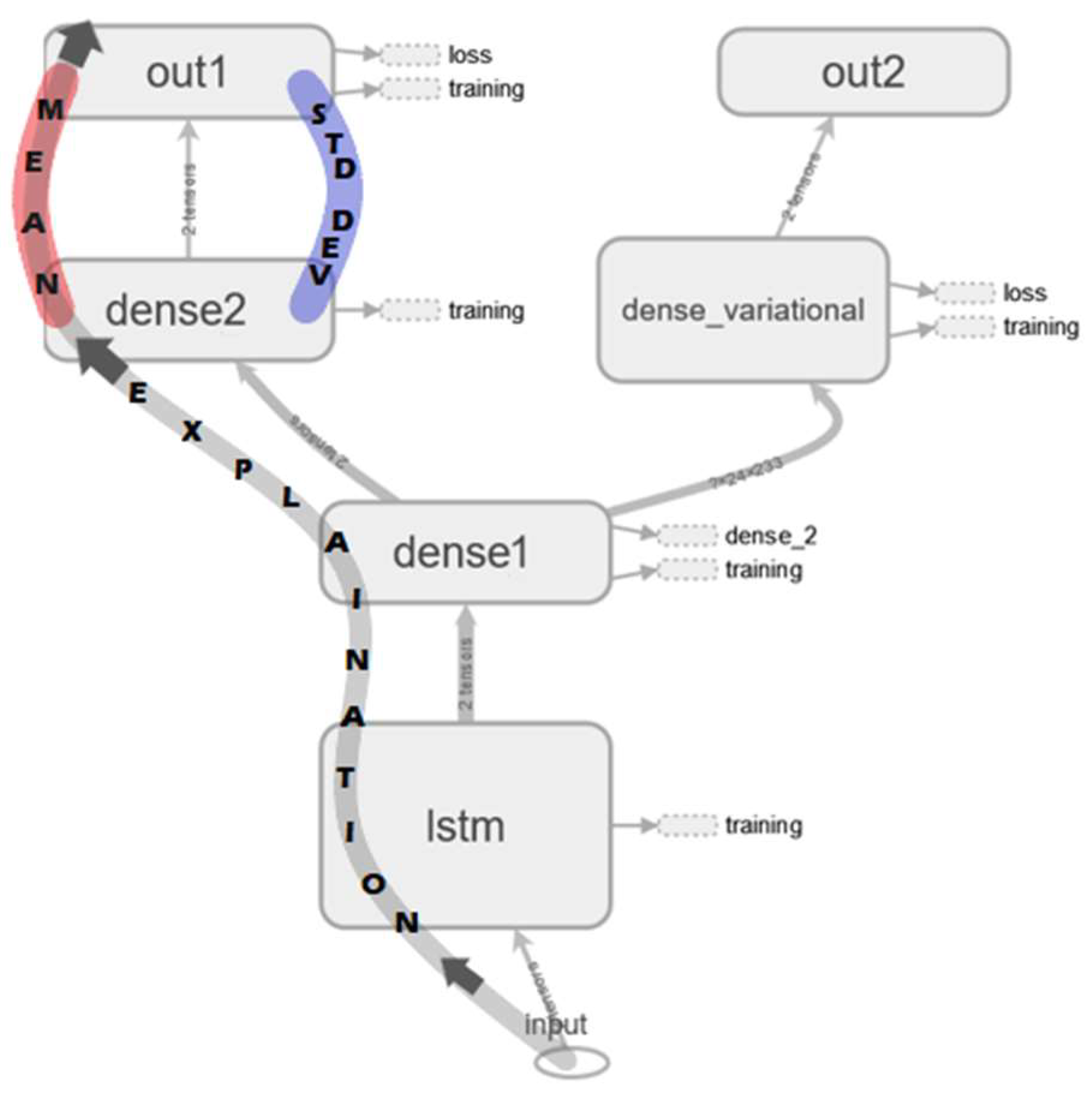
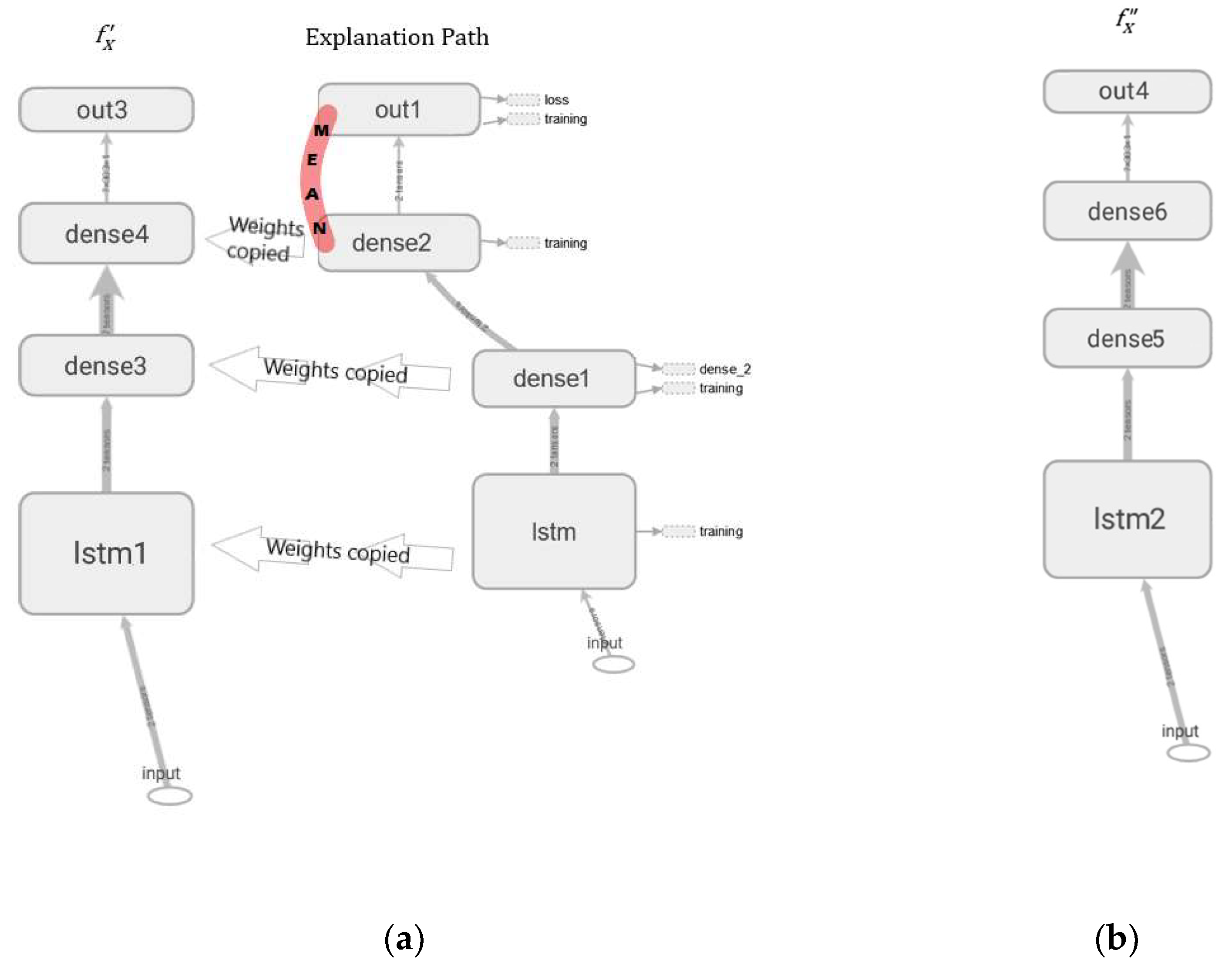
2.1. Multi Output Bayesian LSTM and Uncertainty Quantification Layers

The computational programs were developed using the following system configurations and libraries versions: NVIDIA GeForce GTX 1650 GPU, CUDA version 11.4, Python version 3.7.6, TensorFlow version 2.3.0, TensorFlow GPU version 2.1.0, TensorFlow Probability version 0.11.1, SHAP version 0.39.0, scikit-learn version 0.23.2, SciPy version 1.4.1, seaborn version 0.10.0, MATLAB R2019a, and MATLAB Bayesopt. The data and codes used in this study are openly available at github.com/AhmadNor (accessed on 9 January 2022).
A single input, multi outputs LSTM model was employed for anomaly detection and RUL estimation tasks. The model, denoted by f x , comprises an input layer, where input data are fed, a single LSTM layer, a fully connected or dense layer, and two output layers, such as presented in Figure 3. The LSTM layer produces sequential prediction by employing a gating mechanism to retain important memory or forget negligible ones. This structure enables the accumulation of important information, a crucial ability in anomaly monitoring and degradation tracking tasks. The input data’s matrix multiplication and addition with the weights and bias factors of the model happen in the dense layer. Then, the forecast, altogether with uncertainty, are enabled by the probabilistic nature of the output layers. Both output layers of f x produced a range of predictions which form the prediction distribution rather than scalar point estimates.
Two types of uncertainties are defined in deep learning models. The first type is the AU, linked to noise, acquisition error, and randomness in the dataset. Thus, the first output layer is the AU layer. It learns and predicts, using the sequential output of the LSTM layer as input, the mean and standard deviation that form the output distributions as depicted in layer “dense2” of f x in Figure 3. The predictions’ spread (the prediction distribution width) is the uncertainty measure. The second type is the epistemic uncertainty (EU), corresponding to the uncertainty of the weights of the deep learning model. Thus, the second output layer is the EU layer, also known as the dense variational layer. This layer learns and predicts the posterior distribution of the weights using variational inference by maximizing the evidence lower bound objective stated as
( D , θ ) = (   q ( w | θ )   log ( q ( w | θ )   P ( w ) ) q ( w | θ ) log ( P ( D | w ) )   ) d w
( D , θ ) = KL [ q ( w | θ ) | | P ( w ) ]   E q ( w | θ ) [ log ( P ( D | w ) ) ] ,
where P ( D | w ) is the probability of the occurrence of data D given a model with parameters w . Note that P ( w ) is the prior or the initial distribution of the weights, whereas q ( w | θ ) is the approximated distribution once the training of the deep learning model is completed. The sampled value q ( w | θ ) is the prediction output. The complete calculation of (2) and (3) can be found in Appendix C.

2.2. Minimization of Uncertainties, Anomaly Detection, and RUL Estimation

The normal distribution, a well understood and commonly used probability model, was utilized to describe both types of uncertainties. The AU and EU are represented by the rolling standard deviation of the predicted distribution’s sequence. The only possible way to reduce the AU of the recorded data is by removing their noise. Hence, the data were firstly denoised using the singular value decomposition algorithm following the methodology stated in [52,53]. The denoised data were later utilized to optimize the deep learning hyperparameters with Bayesian hyperparameter optimization (BayesOpt), whose limits are shown in Table A1 in Appendix A [54]. The BayesOpt optimized the model and decreased the EU.
For anomaly detection, the model was trained with healthy data, as it is expected that the AU will show a spike when the model detects an abrupt anomalous observation. This spike, or change-point, was detected using a CUSUM algorithm with a specified control limit C as stated in [55]. Note that C was determined via the prediction’s AU of the healthy data. Given AU stdmax , AU stdmean , and AU stdstd corresponding to the maximum, mean, and standard deviation (std) of the standard deviations of the AUs, respectively, the specified control limit is defined as C = ( AU stdmax   AU stdmean ) / AU stdstd .
Given a sequence y i , , y n of process measurements with mean μ x and standard deviation σ x , the lower and upper cumulative process sums are defined as
u i = { 0 , max ( 0 , u i 1 + y i μ x 1 2 n σ x ) , i = 1 , i > 1 ,
l i = { 0 , min ( 0 , l i 1 + y i μ x + 1 2 n σ x ) , i = 1 , i > 1 ,
where u i and l i stated in (4) and (5) are the lower and upper cumulative process sums.
Deviation is detected at point y j if u j > C σ x or l j < C σ x . For prognostic purpose, the deep learning model was trained with both healthy and degradation data. The trend of the AU reflects the confidence of the model in its prediction. The rising AU trend mirrors a growing uncertainty, while the contrary represents increasing confidence of the deep learning model.

2.3. Model Performance Assesment and SHAP Explainability

The root mean squared error (RMSE) and early prognostic metric were employed for performance assessment. The first metric was applied to evaluate both the anomaly detection and prognostic tasks while the second one was only used for prognostic.
The RMSE was utilized to examine the model’s predictive performance with AU and EU [56]. To obtain a meaningful measure, the mean performance for 100 predictions was calculated. The RMSE measures how spread the errors are between the prediction values and the true values, defined as
RMSE mean = 1 N i = 1 N ( True ( i ) Pred mean ( i ) ) 2 100 ,
where True ( i ) stated in (6) is the true value and Pred mean ( i ) is the predicted value (the mean of predicted distribution). In anomaly detection, i refers to instance i ,   N to the total instances, and True ( i ) and Pred mean ( i ) correspond to the true and predicted mean outputs at instance i , respectively. In prognostic, i refers to asset/machine i , N to the total assets/machine, and True ( i ) and Pred mean ( i ) are the true and predicted mean RUL of asset i , respectively. In addition, we define the early prognostic metric as
S = (   N i = 1 N s i ) 100 ,
where
s i = { e d i 13   1 ,   d i < 0   e d i 10 1 ,   d i > 0 } , d i = ( RUL pred ( i )   RUL true ( i ) ) .
The metric S stated in (7) gives higher score for errors of similar amplitude in early prediction than late prediction, as the former is more important in failure estimation. Note that s i is the individual asset’s prognostic score, which is the individual asset’s prognostic error between the predicted RUL of asset i , RUL pred ( i ) , and the true RUL of asset i , RUL true ( i ) . Here also, the mean of 100 prediction scores of AU and EU were calculated.
The SHAP is a technique to explain any machine learning model’s output mechanism based on game theory [57]. It uses Shapley values to assess the contribution of each feature to the prediction. The formula for the Shapley value is given by
ϕ j ( v a l ) = R { x 1 ,   , x p } \ { x j } | R | ! ( p | R | 1 ) ! p !   ( v a l ( R   { x j } ) v a l ( R ) ) .
The Shapley value of feature j defined in (8), ϕ j , is the average marginal contribution of feature j ’s value over all probable combinations of feature values regarding the prediction. Note that R is a subset of the total p features and x is the instance’s vector to be explained. The prediction for feature values in set R that are marginalized over those excluded from set R is v a l x ( R ) defined as
v a l x ( R ) = f ^ ( x 1 ,   , x p ) d P x R   E X ( f ^ ( X ) )
where E X ( f ^ ( X ) ) expressed in (9) is the expected value of all predictions. The description of the SHAP is provided next. Given the model of explanation, e , the coalition vector, z { 0 , 1 } N , with z = 1 indicating that the feature is present in the coalition, while z = 0 points to the contrary, and N being the maximum coalition size, we have that
e ( z ) = ϕ 0 + j = 1 N ϕ j z j ,
where, as mentioned, ϕ j expressed in (10) is the Shapley value of feature j .
The SHAP can explain both global and local outputs. However, it is not compatible with probabilistic deep learning and only accepts a single output vector for explanation. Thus, a workaround, in the form of a non-probabilistic model labelled as f x , was developed as shown in Figure 4a. Note that f x has the same layers and weights as those figured along the explanation path in f x , except for the weights in dense2 of f x . Here, only the weights corresponding to the mean were used and transferred from f x to f x , while the weights associated with the standard deviation were ignored. The output layer out3 in f x slices only the first value of each sequence vector and arranges them in a single vector for the SHAP explanation.

2.4. Explanation Visualization

Three means of visualization were used for illustrating the local and global explanations, as follows:
(i)
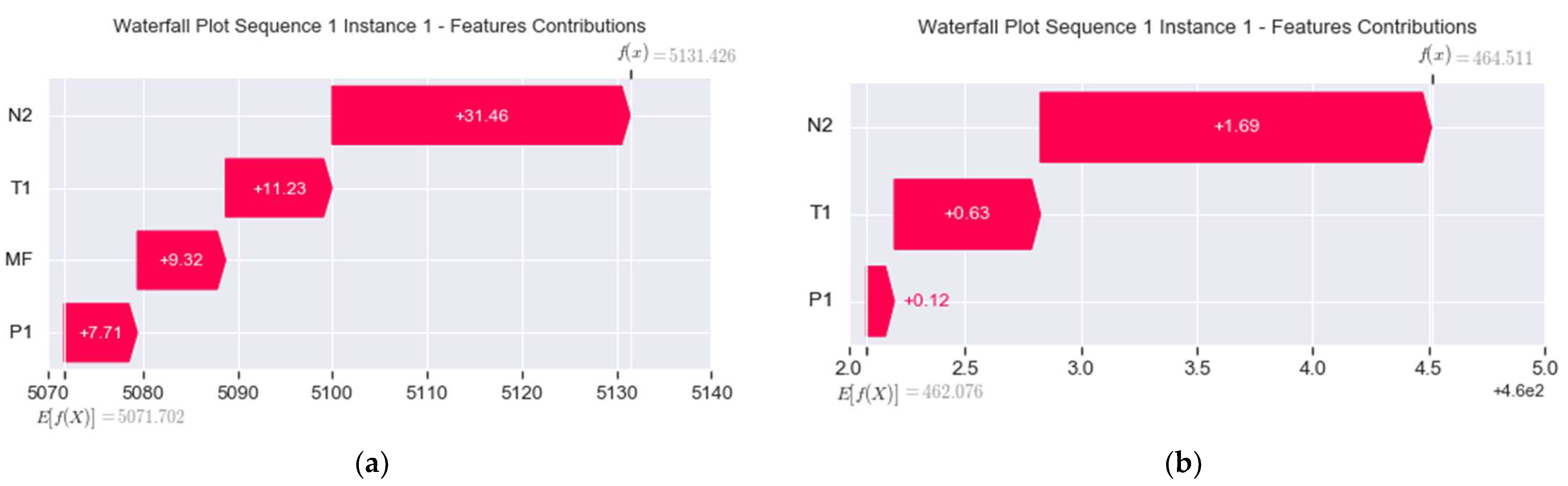
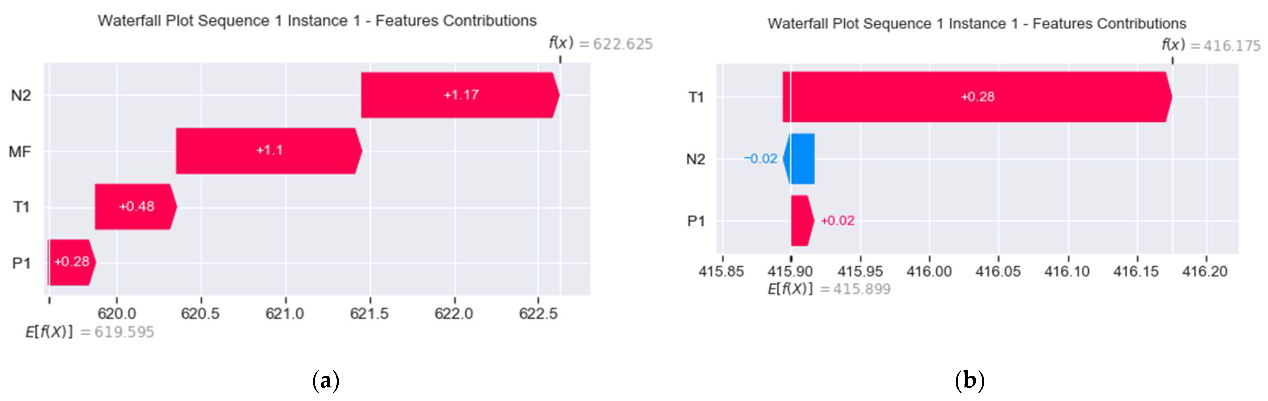
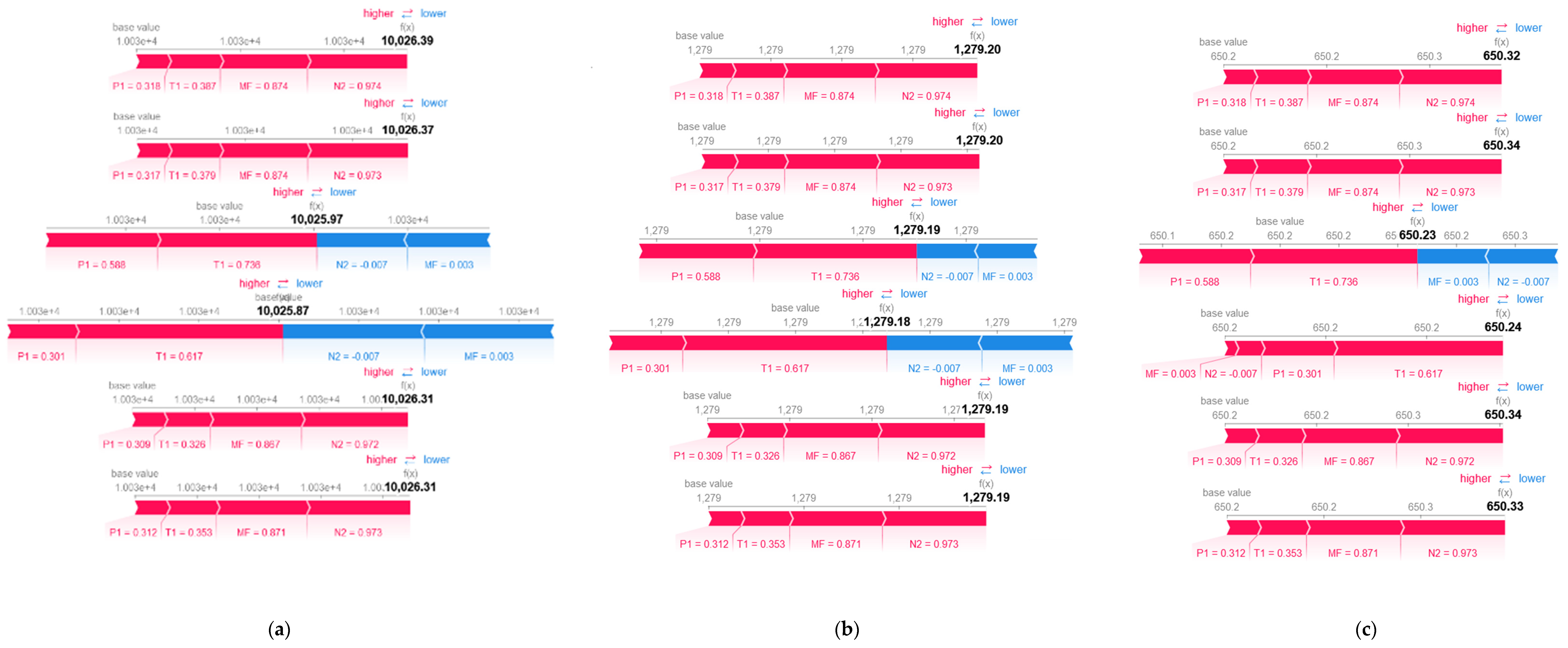
Local: This is based on force and waterfall plots, which highlight the positive or negative forces of features influencing an instance’s output. On the one hand, the force plot shows successive colored bars, where each bar represents a feature contribution. The length of the colored bar represents its force amplitude or impact on the prediction, and the values associated with the features are the normalized values of the features. The red color means that the feature in question is pushing the prediction positively to increase the output value, f ( x ) , while the blue color means that the feature is dragging the prediction negatively to decrease the output. This plot was utilized for explaining anomalous instances. On the other hand, the waterfall plot arranges the feature contribution values in bar-like form according to their force amplitude, where the highest is in the top position, while the lowest is at the bottom spot, forming a waterfall-like pattern. Note that the color’s meaning is the same as before, that is, the direction of the force is clearly shown. This plot was used to verify the local accuracy and consistency properties of the explanation elaborated in the next subsection.
(ii)
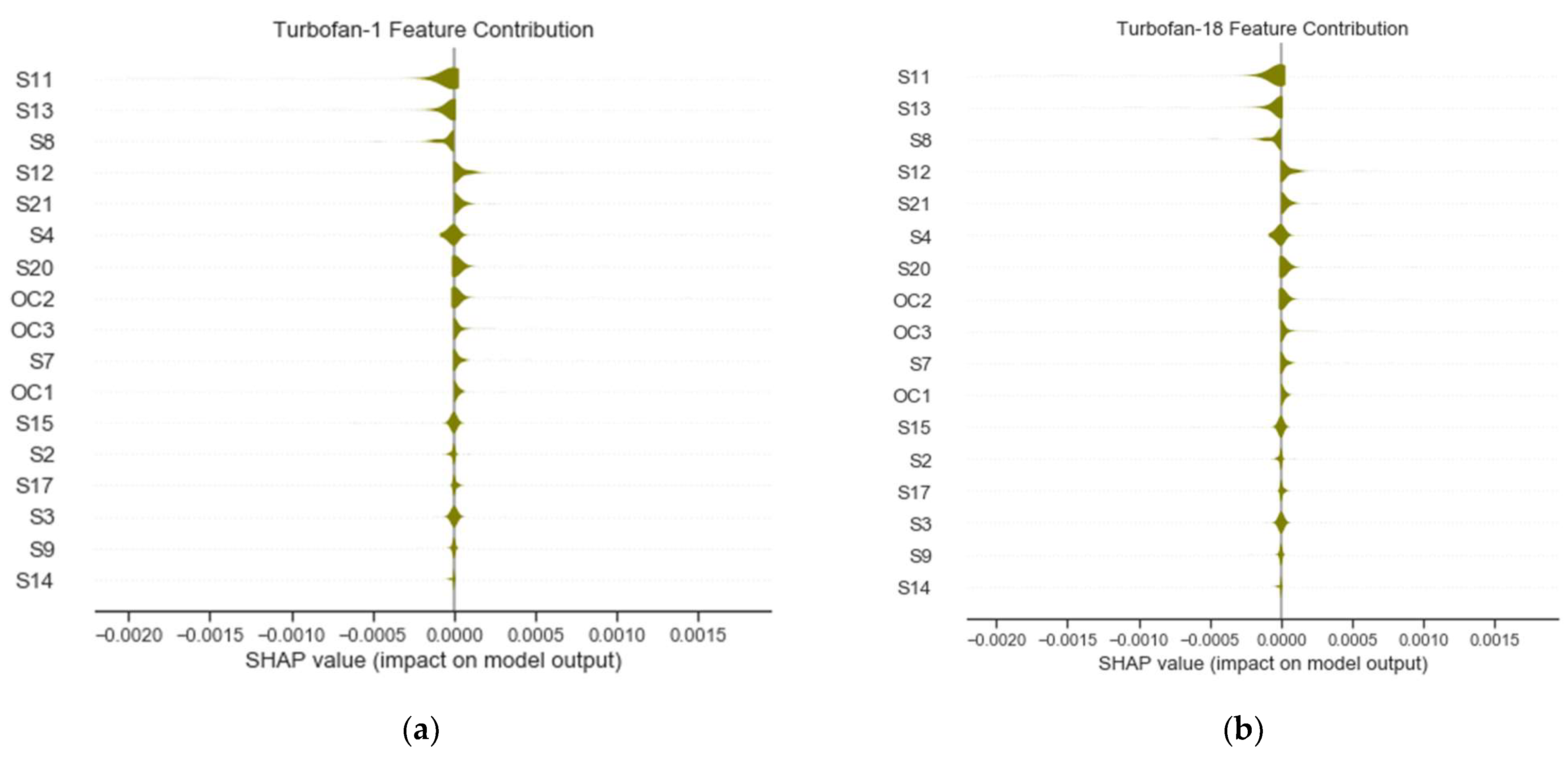
Global: This is based on a summary plot, which highlights the most contributing features in a sequence. The plot arranges the features according to its contributing power and its forces’ directions. Here, the explanation was exploited to enhance the prognostic accuracy by employing only the most contributing features. The model was initially tested with all the features followed by only using 75% of the best of them. Therefore, the performances of the different settings were analyzed and compared with published results.
The first explanation property to be verified was the local accuracy of the SHAP as stated in [58]. It establishes that the sum of the feature contributions, j = 1 N Φ j , is equal to prediction of x or f ( x ) , minus the average prediction, E x ( f ^ ( X ) ) .
From the definition of the SHAP given in (10), posing f ^ ( x ) = e ( z ) and ϕ 0 = E x ( f ^ ( X ) ) , we get that
f ^ ( x ) =   E x ( f ^ ( X ) ) + j = 1 N Φ j x j ,
where Φ j x j , as indicated in (10), is the contribution of feature j , Φ j times whether it is present ( x j = 1 ) or absent ( x j = 0 ) . Hence, j = 1 N Φ j x j is the sum of feature contributions. By setting x j = 1 in (11), the efficiency property of the Shapley values defined in (12) is retrieved. This property was examined using a waterfall plot. Note that
j = 1 N Φ j = f ^ ( x )   E x ( f ^ ( X ) ) .
The second property is consistency, which states that if a model is modified, resulting to either the unchanged or increased marginal contribution of a feature, the Shapley value also follows the marginal contribution’s trend, as defined in [58].
Let v be the complete set of features and v \ j the absence of feature j from the set of features v , for models f and f . Thus, if
f x ( v ) f x ( v \ j )   f x ( v ) f x ( v \ j ) ,
for v   { 0 , 1 } N , then we have that
Φ j ( f , x )     Φ j ( f , x )
where f x ( v )   is calculated from f x and f x ( v ) for the model f x shown in Figure 4b, having the same layers as f x , but with different weights. Observe that f x ( v \ j ) and f x ( v \ j ) are obtained by removing the weights of the feature j from f x and f x , respectively. To calculate the expression presented in (13), a waterfall plot was used for obtaining the values of f x ( v ) , f x ( v \ j ) , f x ( v ) , f x ( v \ j ) and to confirm Φ j ( f , x ) and Φ j ( f , x ) in the inequality formulated in (14).

3. Results

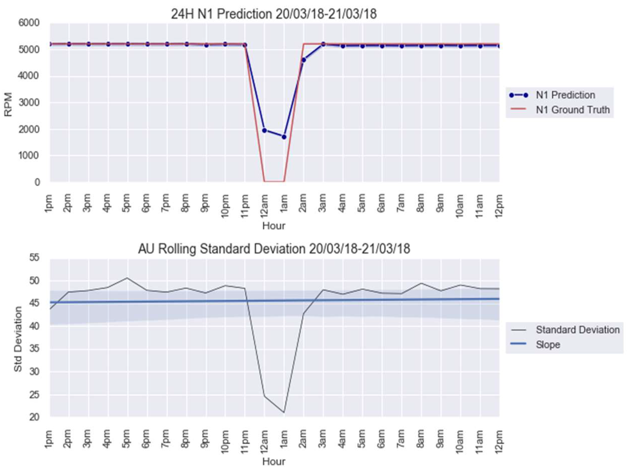
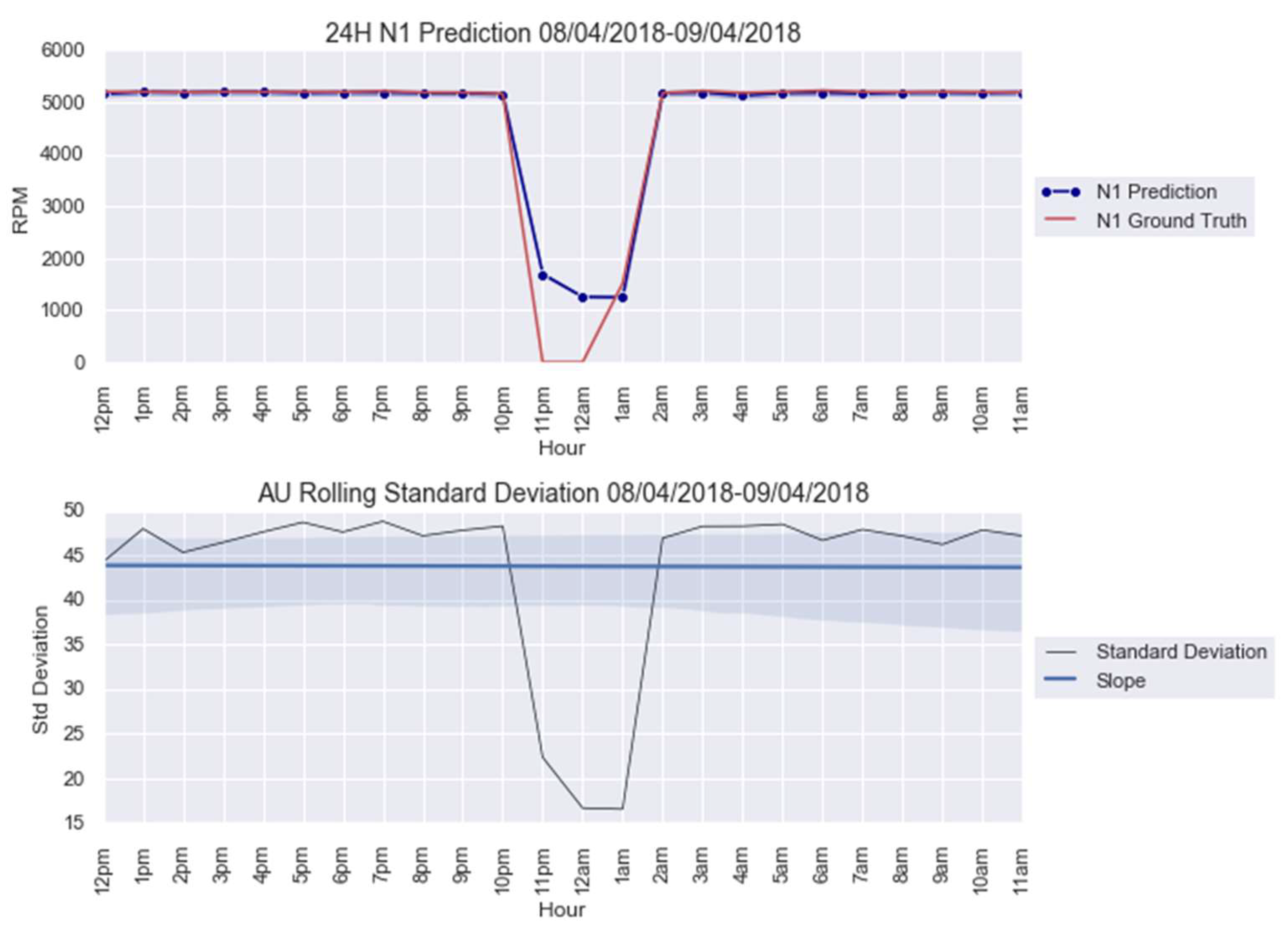
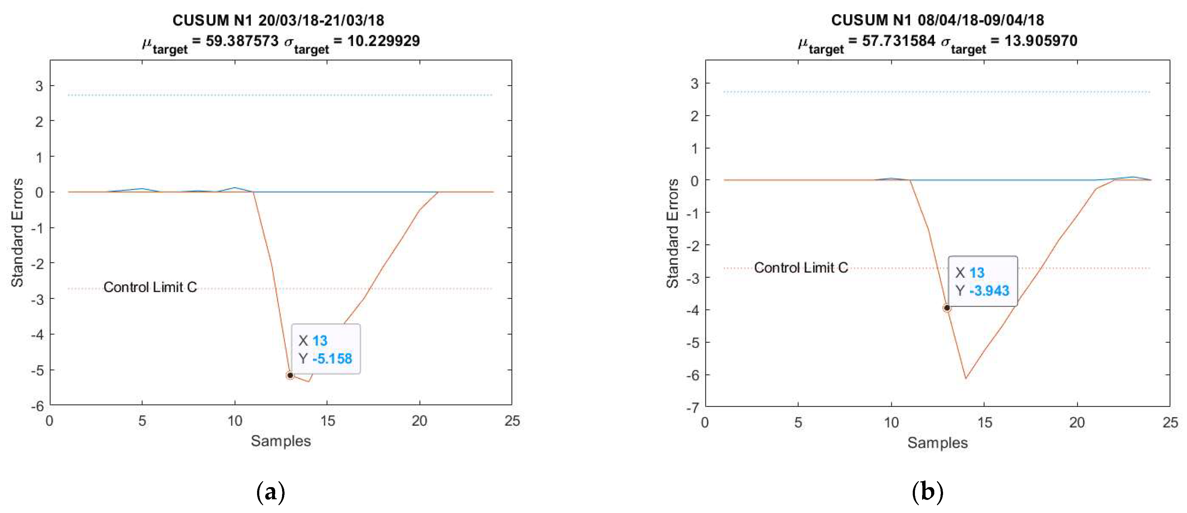
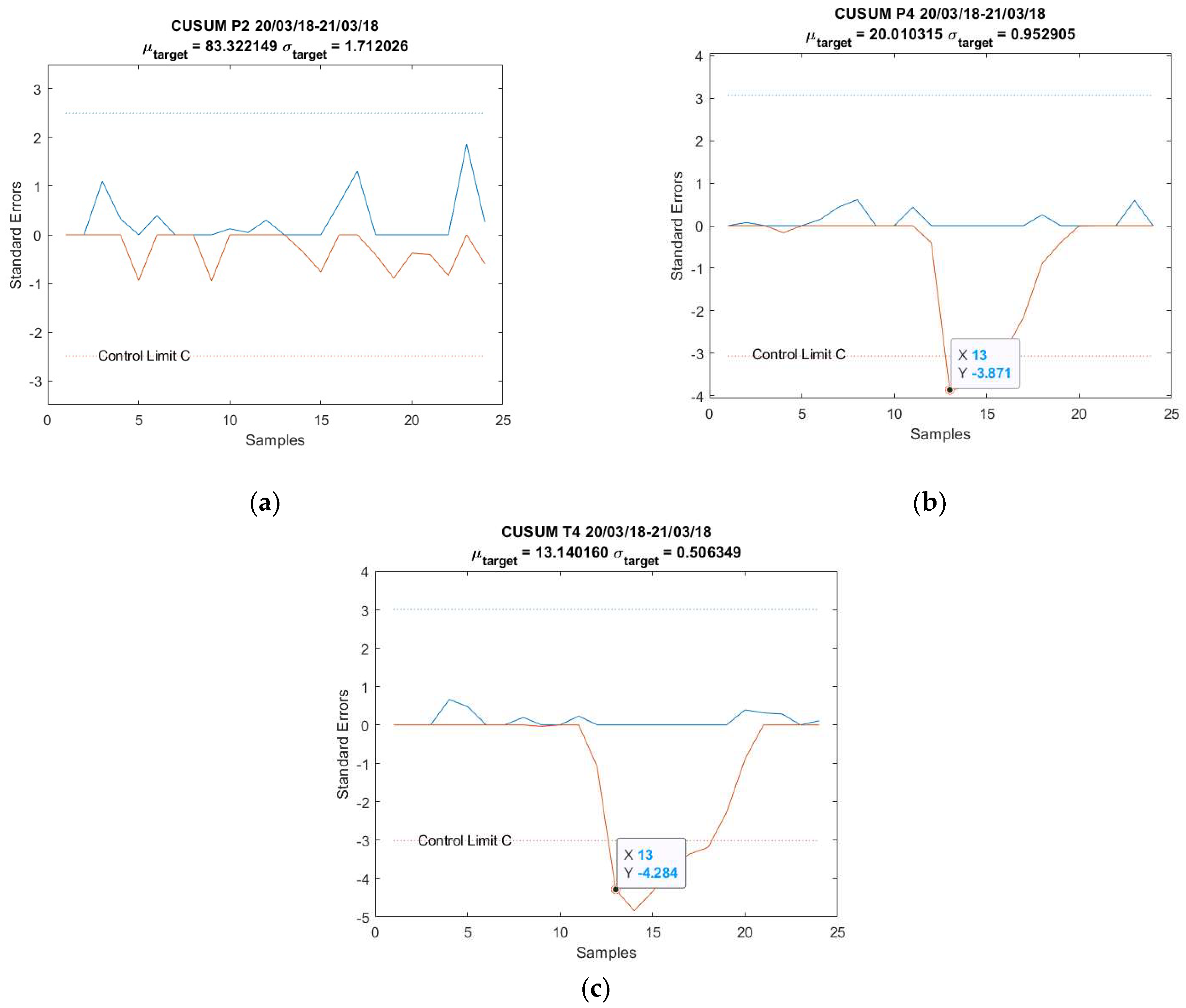
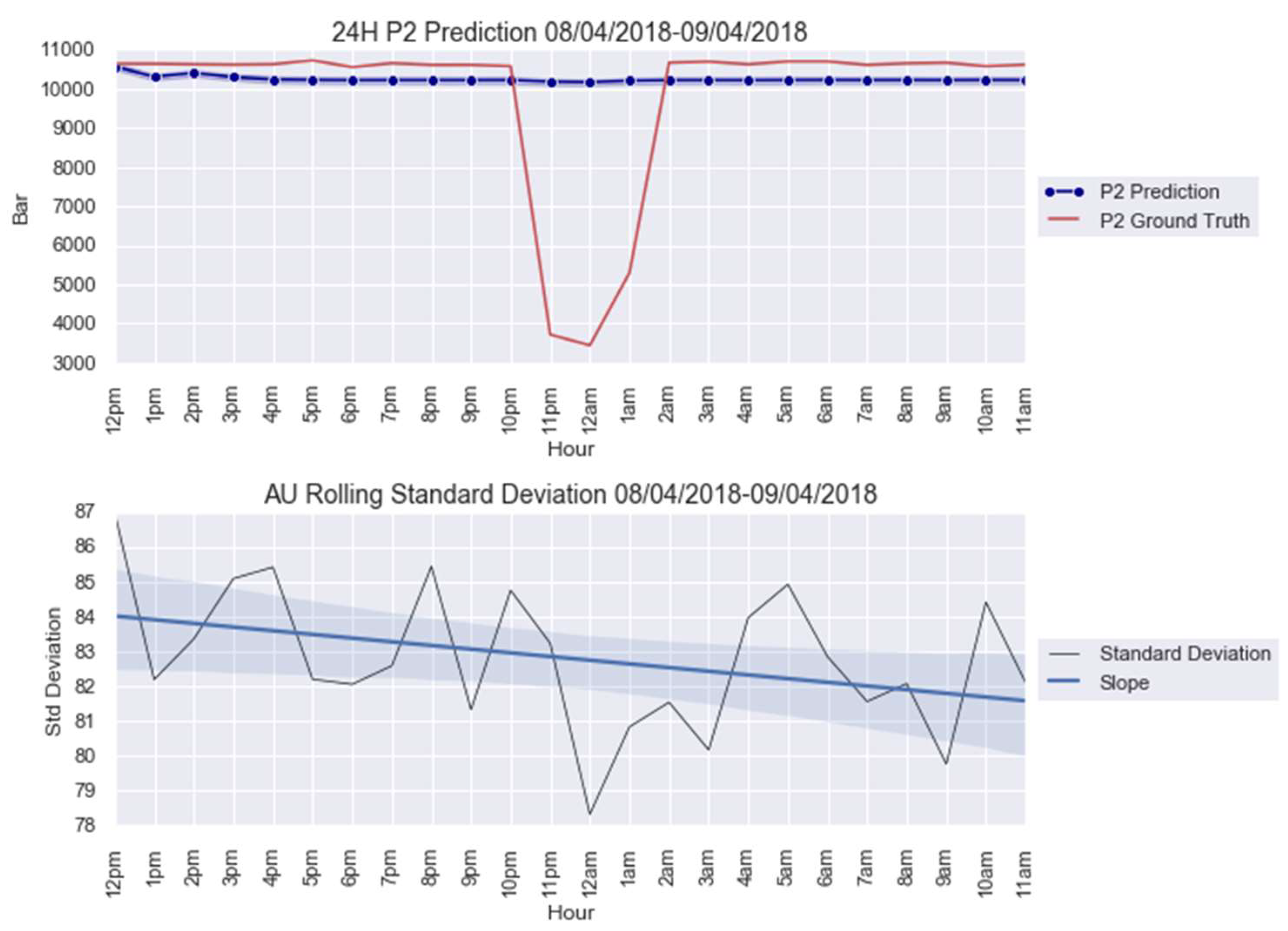
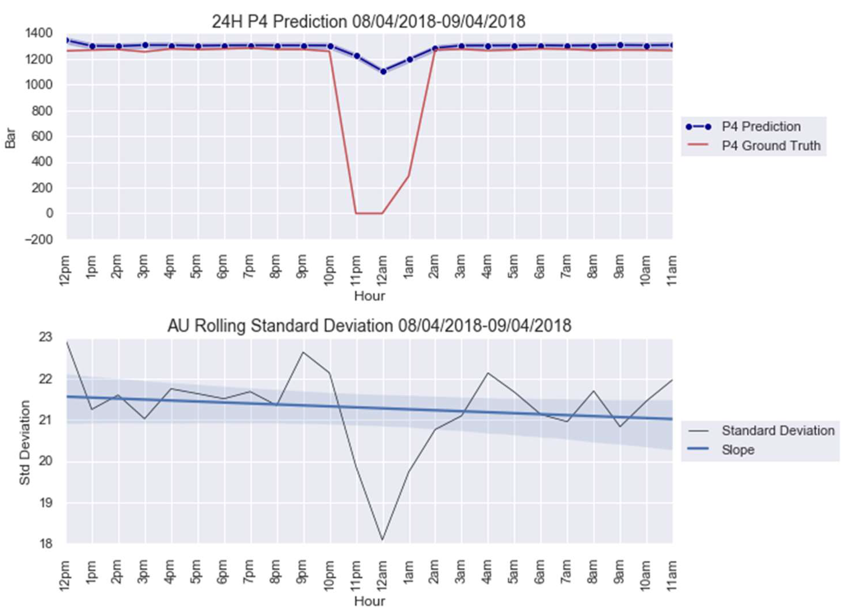
3.1. Case Study 1 from Industry: Real Gas Turbine Anomaly Detection

Data from an 18.8 megawatt-powered, twin-shaft industrial gas turbine from Petronas Angsi Oil Platform in Terengganu, Malaysia, recorded over a one-year period, or 8737 hours, were used in this study. Note that 98 sensor signals, comprising of various pressure, temperature, velocity, and positional readings, make up the largely healthy data. While the features number is overwhelming, only some of them were used in modeling the gas turbine, as indicated in [59]. The inputs and outputs utilized are shown in Table 1 and Table 2, respectively. Four deep learning networks using f x architecture, labelled as Bayes _ LSTM N 1 ,   Bayes _ LSTM P 2 ,   Bayes _ LSTM P 4 , and Bayes _ LSTM T 4 , were fed with all the inputs to predict each output.
First, we preprocessed the data. The anomaly part was separated from the dataset and the healthy part was split for training, validation, and testing datasets as shown in Table 3. Sequence of input and output were set to 24 h. The only abrupt null sensor’s reading instances from 12 a.m. to 1 a.m. on 20 March 2020 to 21 March 2021 and 11 p.m. to 12 a.m. on 8 April 2018 to 9 April 2018 were tested. They were chosen from the anomaly data collection and merged with the neighboring healthy data to put together a sequence of 24 h. Both anomalies were set to be on 12th to 13th instances of the sequences.
The RMSE results of Bayes _ LSTM N 1 ,   Bayes _ LSTM P 2 ,   Bayes _ LSTM P 4 , and Bayes _ LSTM T 4 predictions with both AU and EU are shown in Table 4. The best result comes from Bayes _ LSTM N 1 , where both RMSEs are low while the worst corresponds to the P2 model. The high difference between the training and testing datasets might be the cause of the poor performance of Bayes _ LSTM P 2 . Note that Bayes _ LSTM P 4 produces an interesting outcome, where the RMSE between AU and EU are not in the same order. This result could be improved by extending the BayesOpt evaluations to minimize the EU. Nevertheless, no performance comparison may be done due to the inexistence of a benchmark result.
For an illustration purpose, the anomalies modelled with Bayes _ LSTM N 1 and AU are shown in Figure 5 and Figure 6. The AU anomaly spike on the 12th and 13th instances can be noted in these figures.
Predictions for Bayes _ LSTM P 2 ,   Bayes _ LSTM P 4 , and Bayes _ LSTM T 4 are in Figure A1, Figure A2 and Figure A3 for 20–21 March 2018. In Figure A6, Figure A7 and Figure A8, we report the predictions for 8–9 April 2018, respectively; see Appendix B. The parameters AU stdmax , AU stdmean , AU stdstd , and C calculated from each model are listed in Table 5.
The CUSUM charts for anomalies predicted from Bayes _ LSTM N 1 obtained from the parameters in Table 5 are shown in Figure 7. Note that both AU spikes are detected by the CUSUM method with the formulated control limit C , as it is the case for all the other models, except for Figure A4a; see Appendix B. The CUSUM charts of the anomalies predicted from Bayes _ LSTM P 2 ,   Bayes _ LSTM P 4 , and Bayes _ LSTM T 4 are in Figure A4 for 20–21 March 2018 and Figure A9 for 8–9 April 2018; see Appendix B.
The force plots for the anomalies predicted from Bayes _ LSTM N 1 are shown in Figure 8. The base value is the mean of training data outputs. Only instances 10 to 15 are displayed for illustration purposes. In Figure 8, f ( x ) relates to N 1 ’s gas generator rotational speed in revolutions per minute (RPM). As depicted in Figure 8 as well as Figure A5 and Figure A10 in Appendix B, N 2 is the anomalous feature due to its negative normalized value.
From the figures mentioned, note that N 1 and N 2 influence positively in instance 11, becoming negative in the 12th and 13th instances, except for the T 4 prediction. In addition, positive influence of P 1 and T 1 grows on the 12th and 13th instances compared to previous instances, except for the N 1 prediction. In Figure 8, N 1 and N 2 forces become dominant on the 12th and 13th instances, making the predictions to be less than the base value. In Figure A5 and Figure A10, P 1 and T 1 are generally the major forces, causing the outputs to be greater than the base value. From the illustrations, observe that most features assert positive impact, pushing the output value higher.

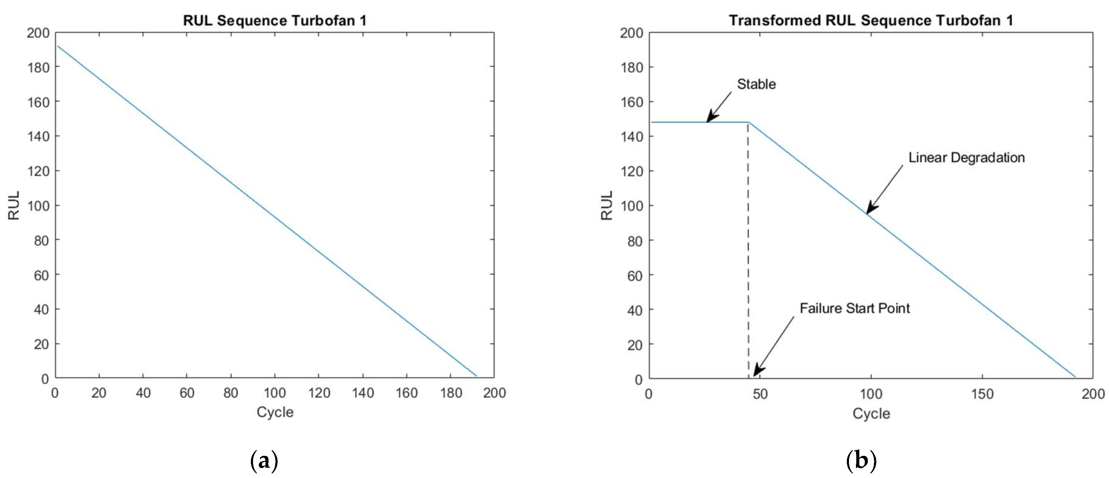
3.2. Case Study 2: Turbofan Engines Failure Prognostic

The FD001 dataset related to NASA turbofan, produced by the Nasa Prognostic Centre (from Ames Research Centre), was used for the prognostic study [60]. These synthetic time series data were generated by modeling a variety of operational scenarios and inserting defects with diverse degrees of deterioration. The original data comprises of training, testing, and true RUL for 100 turbofan engines as summarized in Table 6. Thus, there are 100 turbofan records, referring to turbofans’ health that declined until breakdown after a given cycle, or failure start point (FSP). Note that 21 sensor signals, described in Table A2 of Appendix A, working per cycle and three operating conditions form the recorded data. The operating condition corresponds to diverse operating regimes, a combination of altitude, throttle resolver angle, and Mach number (ratio of object velocity to speed of sound) that conceal the extent of degradation of each turbofan. On top of this, high-level noise is blended to the dataset.
As in case study 1, we first preprocessed the data. Out of the 21 signals, only 14 sensors whose signals’ trends are strictly monotonic were selected as they best represent degradation contrary to irregular and unchanged signals. The total inputs, including three operating conditions, are 17.
A piece-wise linear degradation assumption was adopted, where the RUL is assumed to be stable before the FSP and decreased linearly thereof until failure. In the initial phase, the RUL is equal to the value of the recorded signal’s last cycle and decreases linearly as illustrated for Turbofan 1 in Figure 9a without the FSP. Then, the CUSUM method with C equal to 5 standard deviations was used to calculate the FSPs of the signals of the concerned turbofan. The mean of these FSPs was set as the FSP of the turbofan. The combination of linear degradation obtained earlier and the FSP, forming the final RUL sequence is shown in Figure 9b. The obtained RULs are limited at 50 to ease the model’s generalization.
Note that some testing data with long sequence lengths are associated with very small true RULs that differed from the characteristic of the training data. Hence, it is anticipated that the model will perform more poorly on these abnormal data. The prognostic results of Turbofans 1 and 18 are examined as the former data’s characteristic bore similarity to the training data’s input-output nature while the latter resembles the abnormal data’s trait.
Next, we provide the results with 100% features. The RMSE and score results with AU and EU are presented in Table 7.
The 3D representation of Turbofan 1 prognostic with AU is shown in Figure 10 to provide the full picture of the modeling. As noted in this illustration, the range of prediction or uncertainty decreased along the cycle, signaling growing model’s confidence in its prediction. For the rest of the work, only the 2D presentations are shown.
The 2D depictions of Turbofans 1 and 18 with AU and EU are presented in Figure 11. Looking at the AU rolling standard deviation slope of each prediction, one can observe a decreasing trend for Turbofan 1 and the contrary for Turbofan 18. Hence, the model expresses increasing confidence in the former and decreasing confidence in the latter one. The different AU outcomes are translated by the model’s prognostic outputs that show better performance for Turbofan 1 than for Turbofan 18. In Figure 11, observe that the RUL prediction with AU agrees with the true RUL in the early cycle before showing degradation and failure earlier than the true RUL curve, which is a demanded quality for prognostic modeling. The prediction oscillates at the end of the degradation phase before stabilizing at the failure stage. Meanwhile, a small gap separates the RUL prediction with AU and EU during the early cycle before both seemingly coincide during the degradation phase onward until failure. This is not the case for Turbofan 18, where both prognostics are far off from the true RUL.
The global explanation for 100% features is provided next. The feature contributions and their directions, issued from f x explanation model, are presented in the summary plots in Figure 12. Both plots seem similar, but they differ. One should prioritize choosing the more confident prediction, which is, in this case, Turbofan 1.
Although the top contributing features influenced the predictions negatively, most of the features had a positive impact on the estimates. The features, according to their contributing power, are ordered in Table 8. Note that 75% (13) of the original features, selected to improve the prognostic modeling, are shown in italic characters corresponding to sensors (S11, S13, S8, S12, S21, S4, S20, S7, S15, S2) and operating conditions (OC2, OC3, OC1).
Now, the performance and prognostic results with 75% of the features are reported. The RMSE and score outcomes with the selected features are presented in Table 9. As observed, the RMSE results with AU and EU show drastic improvement from the previous results, with the score, however, being worse. Outcomes for Turbofans 1 and 18 are depicted in Figure 13. The same manifestation of AU slope trends as in previous results is observed, matching the prognostic outcomes. Turbofan 1 modeling shows improvement as the oscillation at the end of the degradation phase decreases before stabilizing in the failure phase. The AU level for Turbofan 18 improves in general from the previous result. In the global explanation for 75% of the features, the features contributions, and their directions, which are mostly having positive impacts in the predictions, are presented in summary plots in Figure 14.
When conducting the performance comparison, only the best RMSE and score with the AU obtained previously are compared being the best published works according to the year of publication [61]. As presented in Table 10, the results are on par with these methods, with the prognostic score occupying the top position amongst all the techniques.
For the illustration purpose, we carry out an explanation evaluation using the waterfall plots of the real-world gas turbine’s T 4 prediction. Note that predictions issued from f x and f x are presented in Figure 15 and Figure 16, respectively. The feature removed is N 1 .
Next, we calculate the local accuracy.
Applying the expression given in (12) on Figure 15a, we obtain:
  • j = 1 N Φ j = 31.46 + 11.23 + 9.32 + 7.71 = 59.72.
  • f ( x )   E x ( f ^ ( X ) ) = 5131.426 − 5071.702 = 59.724 ≈ 59.72.
Now, applying the expression given in (12) on Figure 15b, we obtain:
  • j = 1 N Φ j = 1.69 + 0.63 + 0.12 = 2.44.
  • f ( x )   E x ( f ^ ( X ) ) = 464.511 − 462.076 = 2.435 ≈ 2.44.
Then, applying the expression given in (12) on Figure 16a, we have:
  • j = 1 N Φ j = 1.17 + 1.1 + 0.48 + 0.28 = 3.03.
  • f ( x )   E x ( f ^ ( X ) ) = 622.625 − 619.595 = 3.03.
Hence, applying the expression given in (12) on Figure 16b, we reach:
  • j = 1 N Φ j = 0.28 − 0.02 + 0.02 = 0.28.
  • f ( x )   E x ( f ^ ( X ) ) = 416.175 − 415.899 = 0.276 ≈ 0.28.
Observe that the calculations confirm the local accuracy property of the explanation. Next, we evaluate the consistency property similarly, that is, applying the expression given in (13) on Figure 15 and Figure 16, we obtain that:
  • f x ( v ) = 5131.426; f x ( v \ N 1 ) = 464.511; f x ( v ) f x ( v \ N 1 ) = 4666.915.
  • f x ( v ) = 622.625; f x ( v \ N 1 ) = 416.175; f x ( v ) f x ( v \ N 1 ) = 206.45.
Thus, we reach
  • f x ( v ) f x ( v \ N 1 ) > f x ( v ) f x ( v \ N 1 ) .
Applying the expression given in (14) on Figure 15 and Figure 16, we obtain that:
  • Φ j ( f , x ) = 9.32; Φ j ( f , x ) = 1.1, thus Φ j ( f , x ) > Φ j ( f , x ) .
Therefore, the calculations now confirm the consistency property of the explanation.

4. Discussion

The insights gained from the study as well as its limitation and future opportunities are elaborated in this section.

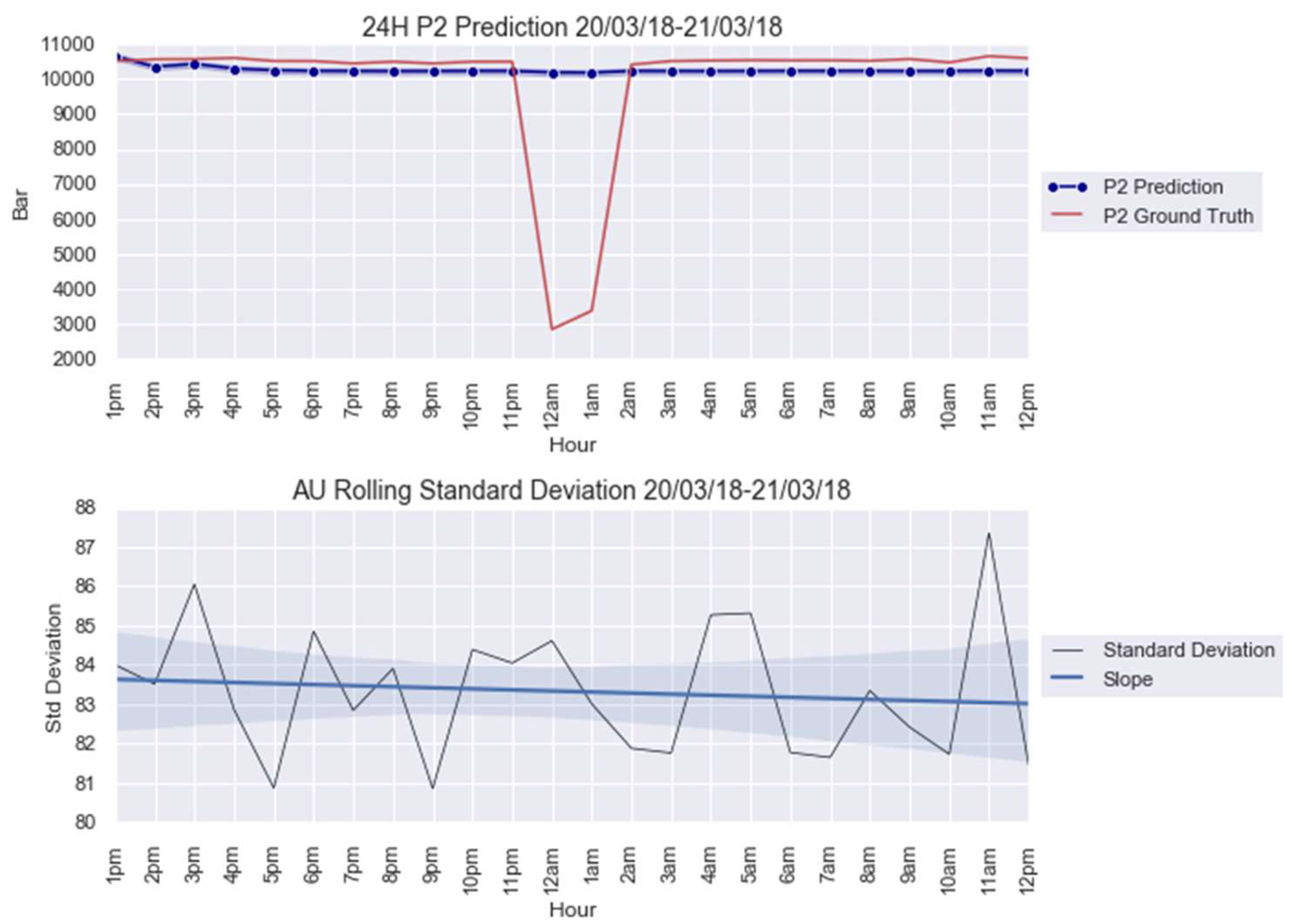
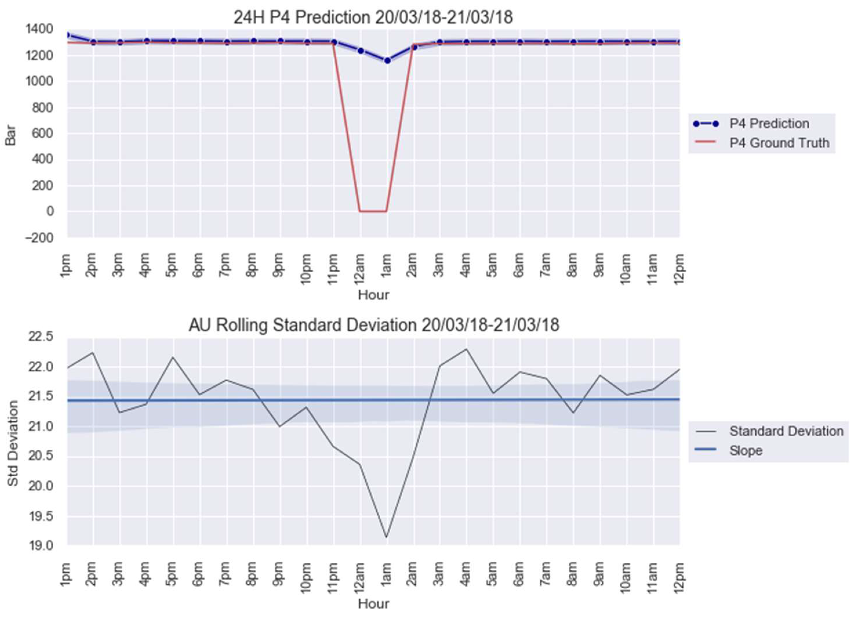
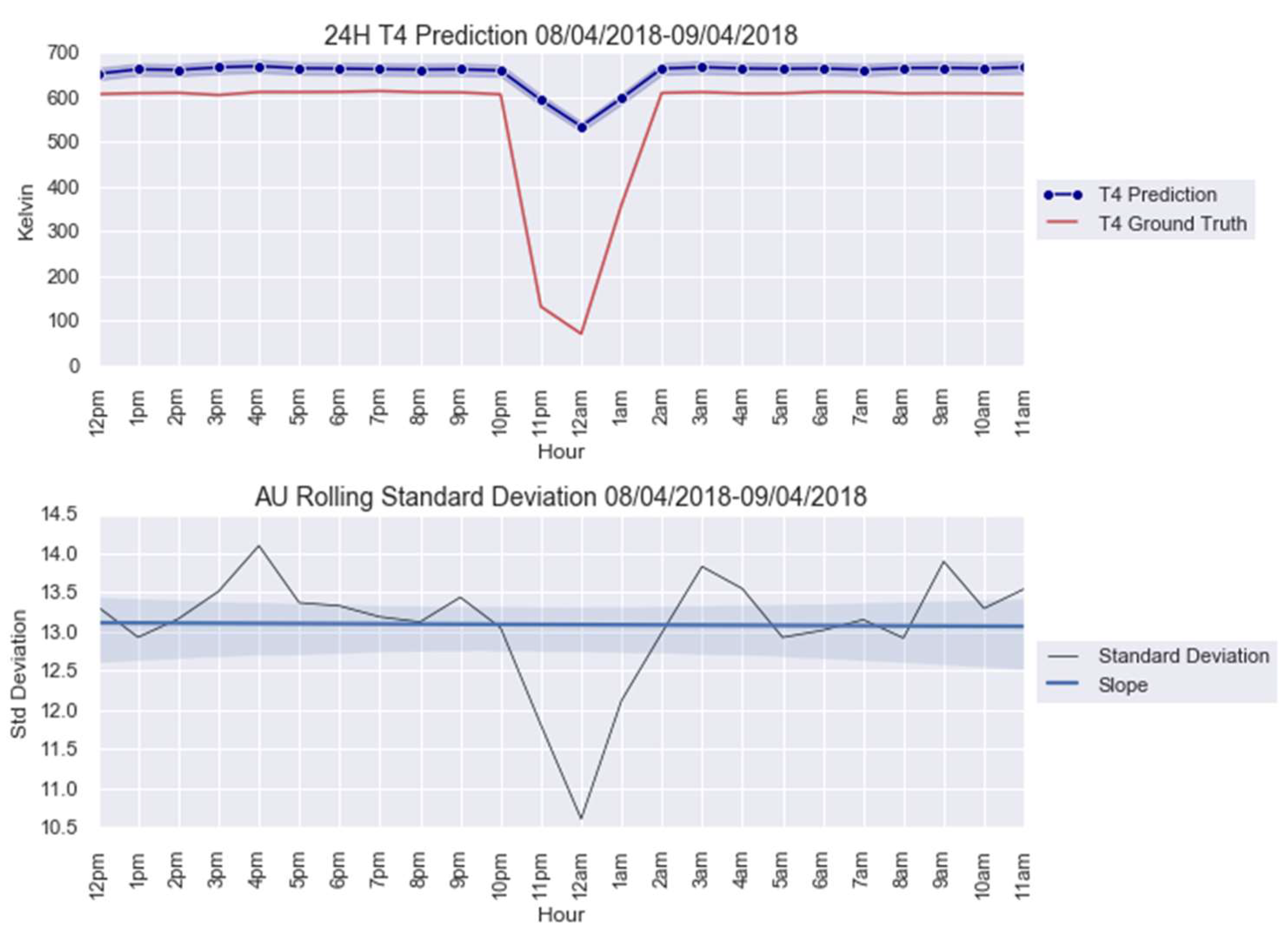
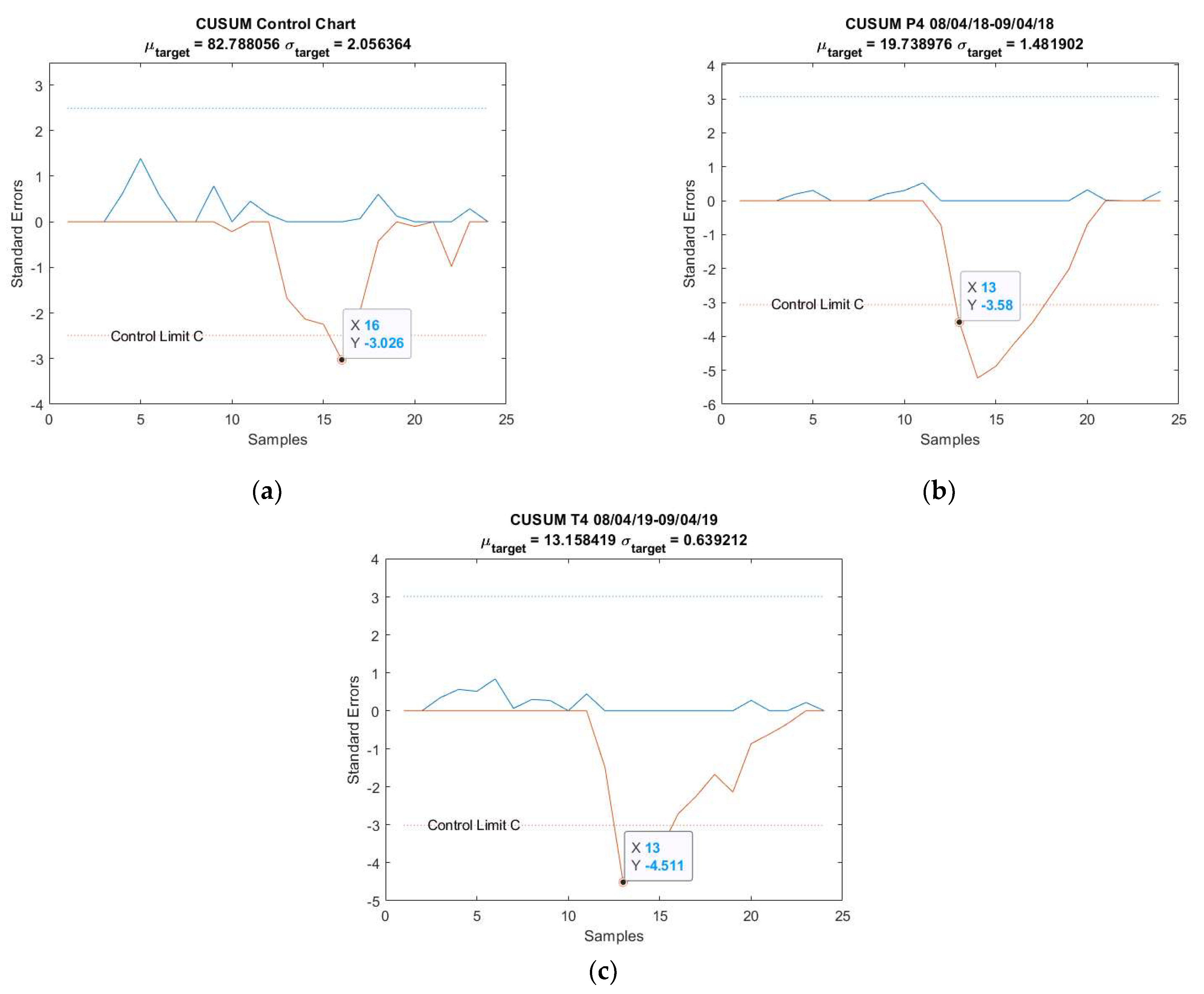
4.1. Anomaly Detection

This paper firstly proposed an anomaly detection framework based on deep learning AU and CUSUM change-point detection. Bayesian deep learning models, capable of generating uncertainties, were trained using only healthy data. Thus, it is expected that the AU, which is influenced by the input data quality, is stable for healthy data and shows abnormality when encountering abrupt anomalies. As demonstrated in Figure 7, Figure A4 and Figure A9, the strategy yielded 87.5% success or 7 out of 8 anomalies detected in the real-world gas turbine dataset. The achievement was partly due to the minimization of AU by the mean of singular value decomposition denoising. As observed, the AU around healthy data prediction is so small because of denoising, except for Figure A4a, where AU variation was too big to be minimized by singular value decomposition denoising. Without this operation beforehand, the anomaly spikes risk is invisible from the rest of the prediction’s AU, hindering effective anomaly detection.
The force plot for local explanation uncovers the dynamic caused by N 2 anomaly to the predictions. Note that N 1 seems to follow N 2 behavior, changing force direction from positive to negative and dragging the prediction lower. The two features’ influence seems amplified in instance 13 due to the consecutive N 2 anomaly. In addition, observe that the positive influences of P 1 and T 1 rose, increasing the prediction. It is also learnt that most features are exerting positive impact that pushed the output value higher. Nonetheless, whether N 2 influenced N 1 ,   P 1 , and T 1 is not certain and could be investigated by other means such as partial dependence plot in the future.
Since the investigation only focused on abrupt anomalies, it is recommended to apply the technique on long consecutive anomalies and examine the generated explanation.
Additionally, this work defined the calculation of control limit C using AU level calculations. However, one can see from Figure 7, Figure A4 and Figure A9 that the anomalies were only identified on the 13th or higher instance, even when the disturbances had already started from the 12th instance. Faster detection could be possible with a proper definition of control limit C . One could lower the limit but a risk of having more false alarms exists, especially when the range of AU is important, such as in Figure A4a. As can be seen in this figure, using 1/3 of C as control limit to identify an anomaly on the 12th instance led to many erroneous detections.

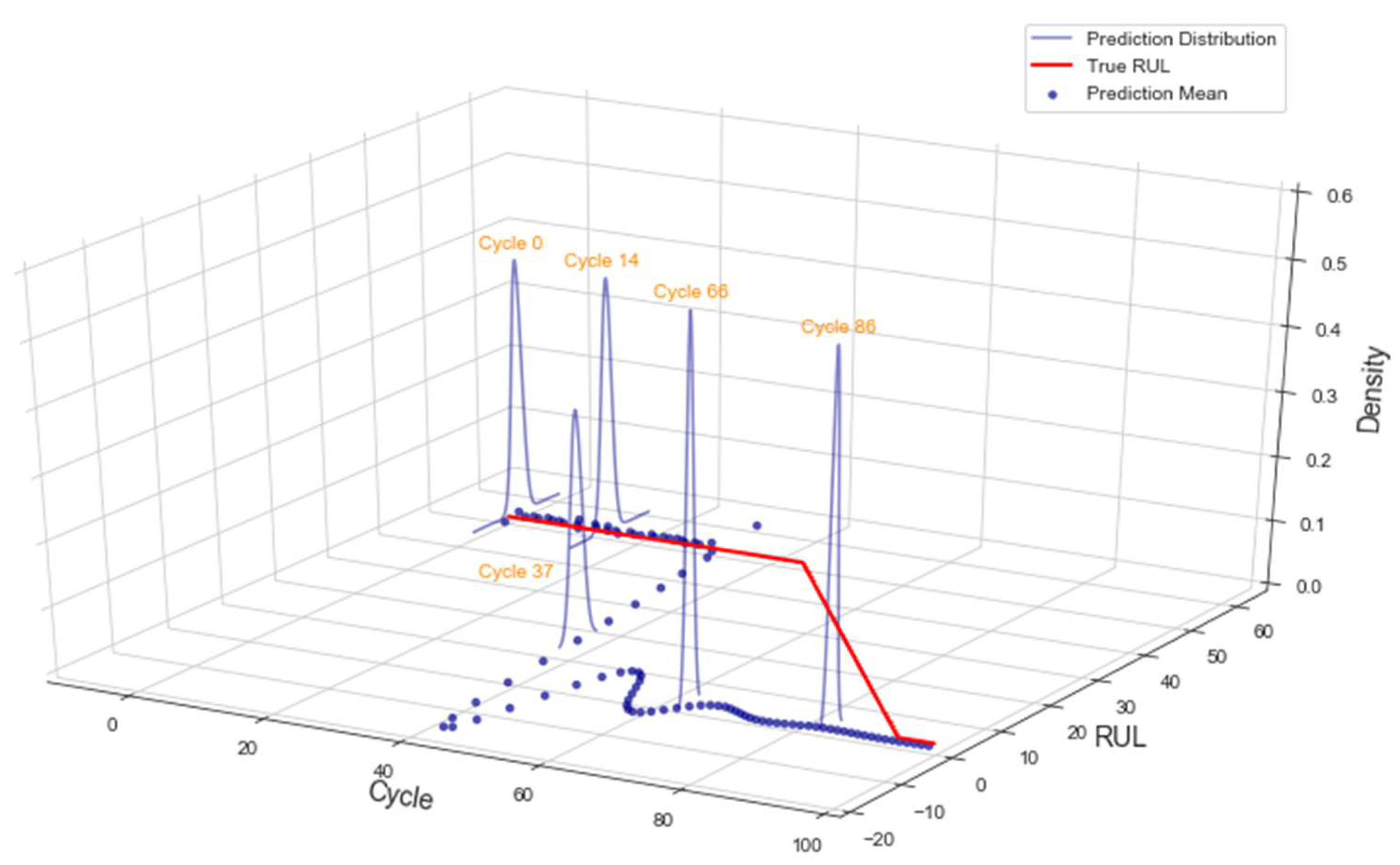
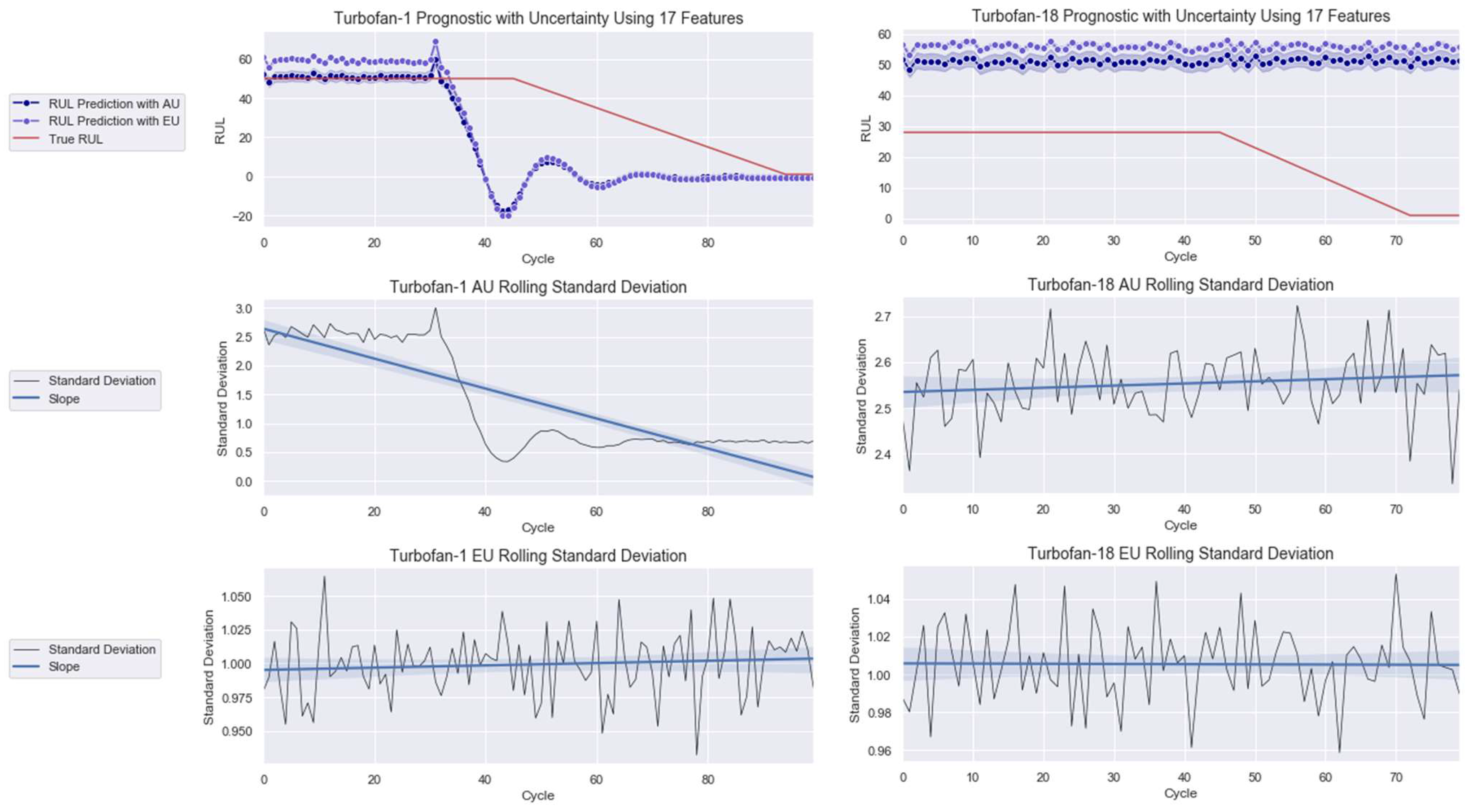
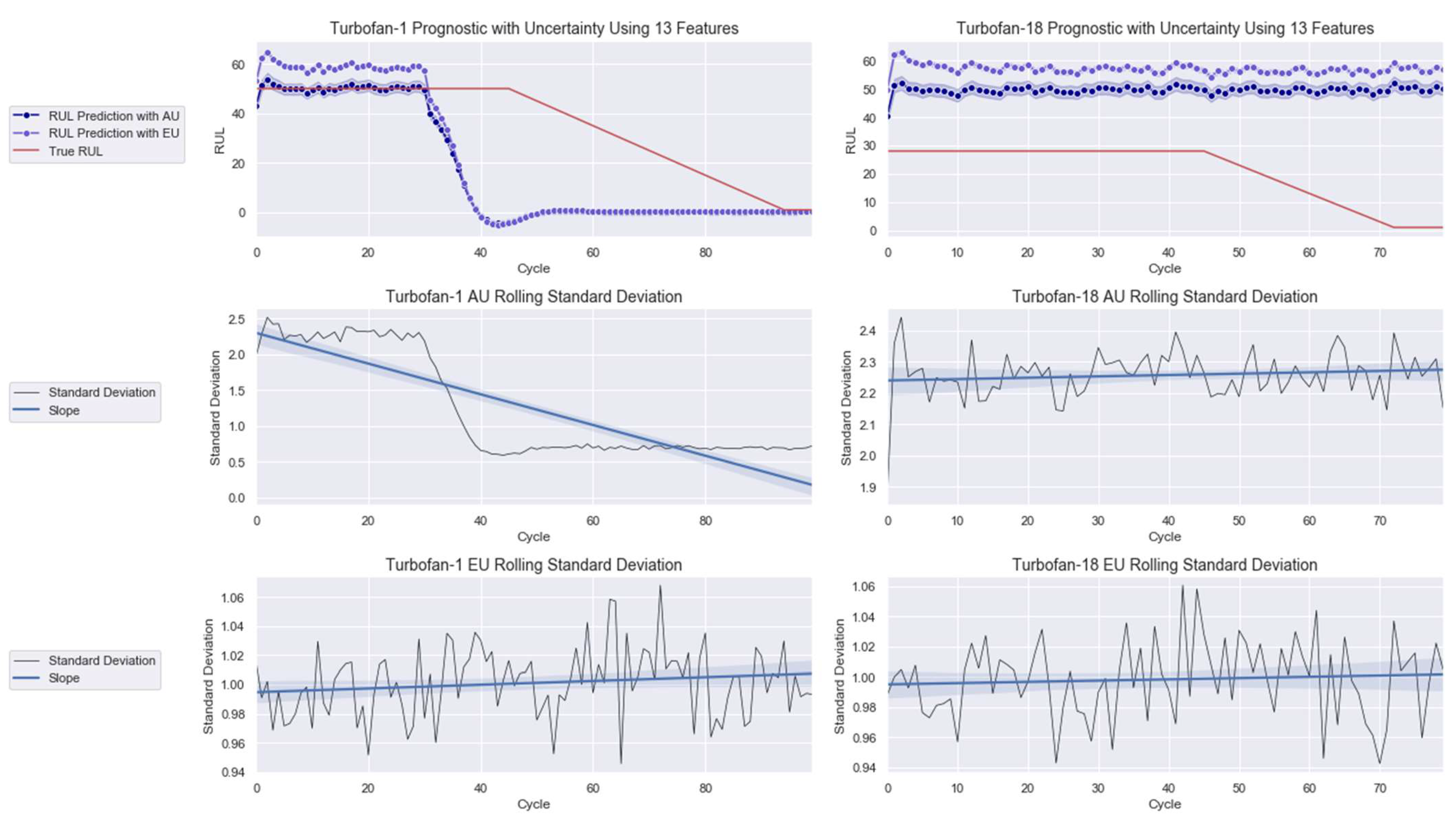
4.2. Failure Prognostic

Secondly, the deep learning model was employed for a failure prognostic purpose. This time, it was fed with both the healthy and failure recorded data. The AU in this task served as a confidence indicator, expressing the uncertainty of the model in its output. Based on the graphical results in Figure 11, Figure 13 and Figure 15, the AU indicator matched all the prognostic modeling, where it increased when the prediction was bad and decreased when the prognostic was good. This feature is vital in failure prediction, especially in the absence of a true RUL. Then, practitioners could judge the quality of the prediction for important decision making.
The global explanation in the form of summary plot helped to improve the performance of the deep learning model. By only using the best contributing features, the RMSE obtained was on par with the best published techniques in this problem. Interestingly, all the operating conditions played important roles in the prediction and made it to the final selection. While the results coming from frequentist models may seems a bit better, this is mainly due to their more complex structures as their designations suggest. The Bayesian deep learning model employed in this work only consisted of a single LSTM and dense layer that limits its nonlinearity modeling power compared to the other methods. Furthermore, the frequentist models could never be utilized in real-life applications, and its usage scope is limited to an experimental purpose as they are devoid of uncertainty quantification. Hence, one could incorporate more complex networks to the existing Bayesian deep learning model in the future to enhance its performance. Other high-performance models, such as transformer, can also be used. Moreover, feature selection could be done from another angle, where features are chosen according to their influence direction rather than their contributing power, to investigate the effect on the performance. The feature selection also improved the AU level using 17 features shown in Figure 11 to using 13 features depicted in Figure 13. This decrease implies that the selection procedure is correct.
The AU indicator provided another dimension in explanation, where it indicated which prediction was reliable before explanation when the XAI approach takes place. This feature enabled the differentiation between explanation of reliable outputs and unreliable ones, helping users and developers to obtain a deeper insight into the AI decision. This distinction facilitates users to prioritize explaining either one of the output types for fast decision making. Time is always a natural constraint in this situation. The prioritization, in turn, will lead to resources optimization for the task at hand. Furthermore, the distinction aided in selecting which global explanation to use for improving the model. Obviously, it would be wiser to choose the explanation from a more confident prediction than a lesser one. Note that the EU level in all the plots hovered around the same range. This is normal as the uncertainty for the weights is fixed once the training was done.

4.3. Safeguarding Security and Explanation Evaluation

Uncertainty quantification excels in minimizing adversarial example risk. This issue arises when new and unseen data, either unintentionally generated or engineered by attackers, is fed to the network. An adversarial example could fool deep learning models. Obviously, frequentist models are unable to detect this abnormality. However, a Bayesian model can signal its presence in the form of rising uncertainty. While this work focused on mechanical failure assumption, it is equally important to investigate failure due to adversarial example as well.
The explanation generated conformed to the local accuracy and consistency properties. The former one also equals to efficiency nature of the Shapley values. Certifying the latter one also means justifying the symmetry and additivity qualities of the Shapley values. The first characteristic asserts that the Shapley values of two features should be equal if their contributions to all probable coalitions are even. The final attribute denotes that for an ensemble prediction, for a specific feature, one can calculate the Shapley value of the feature in each individual ensemble, average them, and obtain the Shapley value for the feature for the whole ensemble.
While the explanation fulfils several demanded general qualities, the need to evaluate an explanation based on PHM criteria, such as security and safety, cost, and time, are still present. This aspect is also echoed in [44]. Therefore, it is crucial for PHM-XAI researchers to develop explanation metrics satisfying the PHM needs.

4.4. Other Aspects

The first dataset employed in this paper comes from a real-world gas turbine. As such, it is expected that failure data to be rare as the gas turbine is well maintained. Thus, the only data exploitable are intermittent anomalies occurring in the system, and we try to explain those abnormalities. This lack of failure data is a known problem in reliability engineering, which resulted in the development of synthetic data. The second dataset is of this latter type, which a is well-known problem in the PHM community and was part of the PHM 08 competition. Recall that the extent of degradation for each turbofan is unknown with high level noise incorporated in the dataset and the failures found are hidden by the effect of various operating conditions. Specifically, dataset FD001 was chosen as it is the most employed dataset in this problem, as indicated in [62], and permits the comparison of the enhanced results with other existing methods. The real-world and synthetic datasets were intentionally used to show that this work is applicable everywhere. Then, the use of both of these datasets is justified. In terms of the practical applications of this work, the objectives of this paper are simply to fulfil some of the research gaps mentioned in [44].
Note that, while trying to obtain the best performance in the problem is an important aspect, it is not part of the objective of this paper. Rather, the SHAP global explanation was used to improve the performance of the model, which is a research gap that was identified in [44]. The performance comparison was only done for the validation purpose. Additionally, for problems related to reliability engineering/industrial maintenance, uncertainty quantification has a higher priority than performance, since the error of prediction can lead to a disastrous effect on productivity, cost, and safety.

4.5. Impacts of the Current Work

Assessing the prediction’s quality should be the first step before its explanation. This assessing is the primary goal of this work. It is the first work in the domain to propose a larger explanation scope through deep learning uncertainties and the XAI approach. Identifying good and bad predictions’ explanations offers more insight to the data, enabling correct analysis that, in turn, leads to accurate decision making.
Uncertainty quantification can assess prediction quality and, thus, should be a mandatory feature in any PHM-XAI work. On top of this, the uncertainty can act as an indicator for an anomaly, adding to its advantage. In addition to its usage flexibility, the potential of SHAP, as a tool for explanation and for enhancing prognostic task’s performance, was also demonstrated in this work. This study could be a catalyst for more researchers in this area exploiting the diverse abilities of SHAP in their forthcoming projects. In addition, our paper provided the first application of explanation evaluation at the XAI method’s level in this field. The sole activity of producing explanation is obviously insufficient.
The quality of the explanation should be examined as it is intended to be reliable for the user. This article could result in more PHM-XAI studies incorporating such a vital assessment in the future. Finally, the paper showed the importance of reducing deep learning uncertainties, a logical process that is usually neglected in investigations related to probabilistic deep learning methods and should be encouraged. As shown in the present research, uncertainties reduction via denoising and hyperparameter optimization procedures proved to be beneficial to the model’s performance.

5. Conclusions

Opacity of AI models constitutes operational and legal risks that could potentially derail investments of AI in the energy and industrial sectors. To promulgate the assimilation of AI in real-world prognostic and health management applications, this article tackles the challenges afflicting PHM-XAI domain, specifically the lack of explanation assessment and uncertainty quantification. PHM tasks relating to anomaly detection and failure prognostic of a gas turbine engine were investigated. The Shapley additive explanation model agnostic approach was employed to generate local and global explanations from a Bayesian deep learning model. The former one was for the anomaly explanation, while the latter one was for the failure prediction. The global explanation was also exploited to improve the prognosis performance. The deep learning model was able to predict with uncertainty whose trend served as anomaly marker that changes intensely with abnormal data. The anomaly detection strategy succeeded in identifying seven out of eight available abnormalities, while the best selected features from the global explanation enhanced prognostic performance to be on par with the best results in the problem. The Shapley additive explanations were validated with the local accuracy and consistency characteristics of explanation.

Author Contributions

Conceptualization A.K.M.N.; methodology A.K.M.N. and V.L.; software, A.K.M.N.; validation, A.K.M.N. and V.L.; formal analysis, A.K.M.N.; investigation, A.K.M.N.; data curation, A.K.M.N.; writing—original draft preparation, A.K.M.N.; writing—review and editing, A.K.M.N. and V.L.; visualization, A.K.M.N.; supervision, S.R.P., M.M. and V.L. All authors have read and agreed to the published version of the manuscript.

Funding

This research was supported partially by Universiti Teknologi Petronas Foundation -YUTP-(A.K.M.N., S.R.P., M.M.) and by project grant Fondecyt 1200525 (V. Leiva) from the National Agency for Research and Development (ANID) of the Chilean government under the Ministry of Science, Technology, Knowledge, and Innovation.

Institutional Review Board Statement

Not applicable.

Informed Consent Statement

Not applicable.

Data Availability Statement

The data and code presented in this study are openly available in github.com/AhmadNor (accessed on 9 January 2022).

Acknowledgments

The authors would like to thank Petronas Bhd. for the data used in this work. The authors would also like to thank the editor and reviewers for their constructive comments which helped improve the presentation of the manuscript.

Conflicts of Interest

The authors declare no conflict of interest.

Appendix A

Table A1. BayesOpt hyperparameters ranges.
ParametersHidden
Units
Fully Connected
Layer Size
Mini Batch
Size
Learning
Rate
Space10 to 100010 to 50026 to 130 5 × 10 4 to
1 × 10 3
Table A2. Turbofan datasets sensors description.
SensorDescriptionUnit
S1Total temperature fan inlet0R
S2Total temperature at low pressure compressor (LPC) outlet0R
S3Total temperature at high pressure compressor (HPC) outlet0R
S4Total temperature at low pressure turbine (LPT) outlet0R
S5Pressure at fan inletPSIA
S6Total pressure in bypass-ductPSIA
S7Total pressure at HPC outletPSIA
S8Physical fan speedRPM
S9Physical core speedRPM
S10Engine pressure ratio (P50/P2)N/A
S11Static pressure at HPC outletPSIA
S12Ratio of fuel flow to Ps30Pps/PSI
S13Corrected fan speedRPM
S14Corrected core speedRPM
S15Bypass ratioN/A
S16Burner fuel-air ratioN/A
S17Bleed enthalpyN/A
S18Demanded fan speedRPM
S19Demanded corrected fan speedRPM
S20HPT coolant bleedlbm/s
S21LPT coolant bleedlbm/s

Appendix B

Figure A1. Bayes _ LSTM P 2 anomaly modeling for 20–21 March 2018.
Mathematics 10 00554 g0a1
Figure A2. Bayes _ LSTM P 4 anomaly modeling for 20–21 March 2018.
Mathematics 10 00554 g0a2
Figure A3. Bayes _ LSTM T 4 anomaly modeling for 20–21 March 2018.
Mathematics 10 00554 g0a3
Figure A4. CUSUM charts anomaly 20–21 March 2018 from (a) Bayes _ LSTM P 2 , (b) Bayes _ LSTM P 4 , and (c) Bayes _ LSTM T 4 .
Mathematics 10 00554 g0a4
Figure A5. Force plots anomaly 20–21 March 2018 from (a) Bayes _ LSTM P 2 , (b) Bayes _ LSTM P 4 , and (c) Bayes _ LSTM T 4 .
Mathematics 10 00554 g0a5
Figure A6. Bayes _ LSTM P 2 anomaly modeling for 8–9 April 2018.
Mathematics 10 00554 g0a6
Figure A7. Bayes _ LSTM P 4 anomaly modeling for 8–9 April 2018.
Mathematics 10 00554 g0a7
Figure A8. Bayes _ LSTM T 4 anomaly modeling for 8–9 April 2018.
Mathematics 10 00554 g0a8
Figure A9. CUSUM charts anomaly 8–9 April 2018 from (a) Bayes _ LSTM P 2 , (b) Bayes _ LSTM P 4 , and (c) Bayes _ LSTM T 4 .
Mathematics 10 00554 g0a9
.
Figure A10. Force plots anomaly 8–9 April 2018 from (a) Bayes _ LSTM P 2 , (b) Bayes _ LSTM P 4 , and (c) Bayes _ LSTM T 4 .
Mathematics 10 00554 g0a10

Appendix C

Appendix C.1. Bayes Theorem

The posterior distribution of the weight can be expressed by the Bayes theorem as
P ( w | D ) = P ( D | w ) P ( w ) P ( D ) = P ( D | w ) P ( w ) P ( D | w ) P ( w ) d w ,
where P ( w | D ) is the posterior distribution, P ( D | w ) is the probability of the occurrence of data D given a model with parameters w , P ( w ) the prior, and P ( D ) the data distribution. Here, P ( w ) is the initial distribution of weights and biases, and D is the training data (input/output pairs). In the full form of the Bayes theorem stated in (1), P ( D ) is intractable to compute due to the number of the parameters that influence the integral. Thus, the only way is to approximate P ( w | D )   [63,64].

Appendix C.2. Variational Inference

(i)
A probability, q ( w | θ ) , is created over the weights w and parameterized by θ as an approximation of P ( w | D ) given by
q ( w | θ ) P ( w | D ) .  
The approximation is done by minimizing the Kullback–Leibler (KL) divergence between q ( w | θ ) and P ( w | D ) . The KL divergence is a measure of similarity between distribution functions that must be minimized. Minimizing the KL divergence results in finding the optimal θ for the network [64] considering
θ opt = argmin θ   KL   [ q ( w | θ )   | | P ( w | D ) ] .
The KL divergence states that
KL   [ q ( x ) P ( x ) ] = q ( x )   log ( q ( x ) P ( x ) ) d x .
Thus, we have
θ o p t = argmin θ q ( w | θ )     log q ( w | θ )   P ( w | D ) d w ,  
θ o p t = argmin θ q ( w | θ )     log q ( w | θ )   P ( D | w ) P ( w ) d w
θ o p t = argmin θ q ( w | θ )   log ( q ( w | θ )   P ( w ) ) q ( w | θ )   log ( P ( D | w ) ) d w
(ii)
From the above, a cost function, which seeks the minimum setting θ , can be developed for
( D , θ ) = (   q ( w | θ )   log ( q ( w | θ )   P ( w ) ) q ( w | θ )   log ( P ( D | w ) ) ) d w .
or
( D , θ ) = KL [ q ( w | θ ) | | P ( w ) ] E q ( w | θ ) [ log ( P ( D | w ) ) ]
with being called the evidence lower bound. Hence, minimizing the cost function equals maximizing the evidence lower bound. As shown in [64], the cost function can be approximated as in (A10) using i t h Monte Carlo sampled weights, w i , drawn from q θ ( w i ) .
( D , θ )   i = 1 n ( log ( q ( w i | θ ) ) log ( P ( w i ) ) log ( P ( D | w i ) ) ) .
(iii)
Then, during backpropagation, every time a forward pass is performed, this cost function is evaluated with sampled weights. In turn, backward pass updates the weights. This iteration is conducted until the training is over. To perform backpropagation through distribution, the local reparameterization trick introduced in [65] for the variational autoencoder is employed.

References

  1. Monett, D.; Lewis, C.W. Getting Clarity by Defining Artificial Intelligence—A Survey; Studies in Applied Philosophy, Epistemology and Rational Ethics; Springer: Cham, Switzerland, 2018; pp. 212–214. [Google Scholar] [CrossRef]
  2. European Commision’s High Level Expert Group on Artificial Intelligence. A Definition of AI: Main Capabilities and Scientific Disciplines. Futurium: Your Voices, Our Future. Available online: ec.europa.eu/futurium/en/system/files/ged/ai_hleg_definition_of_ai_18_december_1.pdf (accessed on 22 December 2021).
  3. European Commission, Executive Agency for Small and Medium-Sized Enterprises. Artificial Intelligence: Critical Industrial Applications: Report on Current Policy Measures and Policy Opportunities. Available online: www.data.europa.eu/doi/10.2826/47005 (accessed on 22 December 2021).
  4. Deloitte. Scenarios and Potentials of AI’s Commercial Application in China. Intelligence Driven by Innovation—Deloitte Released China AI Industry Whitepaper. Available online: www2.deloitte.com/content/dam/Deloitte/cn/Documents/innovation/deloitte-cn-innovation-ai-whitepaper-en-191212.pdf (accessed on 22 December 2021).
  5. Anantrasirichai, N.; Bull, D. Artificial intelligence in the creative industries: A review. Artif. Intell. Rev. 2021, 55, 589–656. [Google Scholar] [CrossRef]
  6. Petit, N. Artificial Intelligence and automated law enforcement: A review paper. SSRN Electron. J. 2018. [Google Scholar] [CrossRef]
  7. Raimundo, R.; Rosário, A. The impact of artificial intelligence on Data System Security: A literature review. Sensors 2021, 21, 7029. [Google Scholar] [CrossRef] [PubMed]
  8. Bates, D.W.; Levine, D.; Syrowatka, A.; Kuznetsova, M.; Craig, K.J.; Rui, A.; Jackson, G.P.; Rhee, K. The potential of artificial intelligence to improve patient safety: A scoping review. NPJ Digit. Med. 2021, 4, 54. [Google Scholar] [CrossRef] [PubMed]
  9. Qiu, S.; Liu, Q.; Zhou, S.; Wu, C. Review of artificial intelligence adversarial attack and defense technologies. Appl. Sci. 2019, 9, 909. [Google Scholar] [CrossRef] [Green Version]
  10. Momade, M.H.; Durdyev, S.; Estrella, D.; Ismail, S. Systematic review of application of artificial intelligence tools in architectural, engineering and construction. Front. Eng. Built Environ. 2021, 1, 203–216. [Google Scholar] [CrossRef]
  11. Buczynski, W.; Cuzzolin, F.; Sahakian, B. A review of machine learning experiments in equity investment decision-making: Why most published research findings do not live up to their promise in real life. Int. J. Data Sci. Anal. 2021, 11, 221–242. [Google Scholar] [CrossRef]
  12. Jung, D.; Choi, Y. Systematic review of machine learning applications in mining: Exploration, exploitation, and reclamation. Minerals 2021, 11, 148. [Google Scholar] [CrossRef]
  13. Bustos, N.; Tello, M.; Droppelmann, G.; Garcia, N.; Feijoo, F.; Leiva, V. Machine learning techniques as an efficient alternative diagnostic tool for COVID-19 cases. Signa Vitae 2022, 18, 23–33. [Google Scholar]
  14. Mahdi, E.; Leiva, V.; Mara’Beh, S.; Martin-Barreiro, C. A new approach to predicting cryptocurrency returns based on the gold prices with support vector machines during the COVID-19 pandemic using sensor-related data. Sensors 2021, 21, 6319. [Google Scholar] [CrossRef]
  15. Ma, L.; Zhang, Y.; Leiva, V.; Liu, S.; Ma, T. A new clustering algorithm based on a radar scanning strategy with applications to machine learning data. Expert Syst. Appl. 2022, 191, 116143. [Google Scholar] [CrossRef]
  16. Palacios, C.A.; Reyes-Suarez, J.A.; Bearzotti, L.A.; Leiva, V.; Marchant, C. Knowledge discovery for higher education student retention based on data mining: Machine learning algorithms and case study in Chile. Entropy 2021, 23, 485. [Google Scholar] [CrossRef] [PubMed]
  17. Deng, L. Achievements and Challenges of Deep Learning. Available online: www.microsoft.com/en-us/research/publication/achievements-and-challenges-of-deep-learning (accessed on 22 December 2021).
  18. Nazmus Saadat, M.; Shuaib, M. Advancements in deep learning theory and applications: Perspective in 2020 and beyond. Adv. Appl. Deep. Learn. 2020, 3. [Google Scholar] [CrossRef]
  19. Sejnowski, T.J. The unreasonable effectiveness of deep learning in artificial intelligence. Proc. Natl. Acad. Sci. USA 2020, 117, 30033–30038. [Google Scholar] [CrossRef] [Green Version]
  20. Dai, Z.; Liu, H.; Le, Q.V.; Tan, M. Coatnet: Marrying convolution and attention for all data sizes. arXiv 2021, arXiv:2106.04803. [Google Scholar]
  21. Rao, A.S.; Verweji, G. Sizing the Prize: What’s the Real Value of AI for Your Business and How Can You Capitalise? Available online: www.pwc.com/gx/en/news-room/docs/report-pwc-ai-analysis-sizing-the-prize.pdf (accessed on 10 January 2022).
  22. Arnold, Z.; Rahkovsky, I.; Huang, T. Tracking AI Investment: Initial Findings from the Private Markets; Center for Security and Emerging Technology: Washington, DC, USA, 2020. [Google Scholar] [CrossRef]
  23. PwC. Leveraging the Upcoming Disruptions from AI and IOT. Available online: www.pwc.com/gx/en/industries/tmt/publications/ai-and-iot.html (accessed on 22 December 2021).
  24. World Intellectual Property Organization. WIPO Technology Trends 2019—Artificial Intelligence. Available online: www.wipo.int/publications/en/details.jsp?id=4386 (accessed on 10 January 2022).
  25. Dernis, H.; Gkotsis, P.; Grassano, N.; Nakazato, S.; Squicciarini, M.; van Beuzekom, B.; Vezzani, A. World Corporate Top R&D Investors: Shaping the Future of Technologies and of AI; A Joint JRC and OECD Report. EUR 29831 EN. JRC Work. Pap.; Joint Research Centre: Ispra, Italy, 2019. [Google Scholar] [CrossRef]
  26. Arnold, Z.; Toner, H. AI Accidents: An Emerging Threat. Center for Security and Emerging Technology; Center for Security and Emerging Technology (CSET): Washington, DC, USA, 2021. [Google Scholar] [CrossRef]
  27. McGregor, S. Preventing repeated real world ai failures by cataloging incidents: The AI incident database. arXiv 2021, arXiv:2011.08512. [Google Scholar]
  28. Chagal-Feferkorn, K. AI Regulation in the World. A Quarterly Update. AI and Regulation. Available online: techlaw.uottawa.ca/sites/techlaw.uottawa.ca/files/ai-regulation-in-the-world_2020_q4_final.pdf (accessed on 22 December 2021).
  29. Gunning, D.; Vorm, E.; Wang, J.Y.; Turek, M. DARPA’s explainable AI program: A retrospective. Appl. AI Lett. 2021, 2, e61. [Google Scholar] [CrossRef]
  30. Streich, J.; Romero, J.; Gazolla, J.G.; Kainer, D.; Cliff, A.; Prates, E.T.; Brown, J.B.; Khoury, S.; Tuskan, G.A.; Garvin, M.; et al. Can exascale computing and explainable artificial intelligence applied to plant biology deliver on the United Nations sustainable development goals? Curr. Opin. Biotechnol. 2020, 61, 217–225. [Google Scholar] [CrossRef] [PubMed]
  31. Bussmann, N.; Giudici, P.; Marinelli, D.; Papenbrock, J. Explainable AI in fintech risk management. Front. Artif. Intell. 2020, 3, 26. [Google Scholar] [CrossRef]
  32. Tjoa, E.; Guan, C. A survey on explainable artificial intelligence: Toward medical XAI. IEEE Trans. Neural Netw. Learn. Syst. 2021, 32, 4793–4813. [Google Scholar] [CrossRef]
  33. Chen, K.; Hwu, T.; Kashyap, H.J.; Krichmar, J.L.; Stewart, K.; Xing, J.; Zou, X. Neurorobots as a means toward neuroethology and explainable AI. Front. Neurorob. 2020, 14, 570308. [Google Scholar] [CrossRef] [PubMed]
  34. Payrovnaziri, S.N.; Chen, Z.; Rengifo-Moreno, P.; Miller, T.; Bian, J.; Chen, J.H.; Liu, X.; He, Z. Explainable artificial intelligence models using real-world electronic health record data: A systematic scoping review. J. Am. Med. Inform. Assoc. 2020, 27, 1173–1185. [Google Scholar] [CrossRef] [PubMed]
  35. Barredo Arrieta, A.; Díaz-Rodríguez, N.; Del Ser, J.; Bennetot, A.; Tabik, S.; Barbado, A.; Garcia, S.; Gil-Lopez, S.; Molina, D.; Benjamins, R.; et al. Explainable artificial intelligence: Concepts, taxonomies, opportunities and challenges toward responsible AI. Inf. Fusion 2020, 58, 82–115. [Google Scholar] [CrossRef] [Green Version]
  36. Adadi, A.; Berrada, M. Peeking inside the black-box: A survey on explainable artificial intelligence. IEEE Access 2018, 6, 52138–52160. [Google Scholar] [CrossRef]
  37. Linardatos, P.; Papastefanopoulos, V.; Kotsiantis, S. Explainable AI: A review of machine learning interpretability methods. Entropy 2020, 23, 18. [Google Scholar] [CrossRef] [PubMed]
  38. Sheppard, J.W.; Kaufman, M.A.; Wilmering, T.J. IEEE standards for prognostics and health management. IEEE Aerosp. Electron. Syst. Mag. 2008, 24, 97–103. [Google Scholar]
  39. Thudumu, S.; Branch, P.; Jin, J.; Singh, J. A comprehensive survey of anomaly detection techniques for high dimensional big data. J. Big Data 2020, 7, 42. [Google Scholar] [CrossRef]
  40. Aykroyd, R.G.; Leiva, V.; Ruggeri, F. Recent developments of control charts, identification of big data sources and future trends of current research. Technol. Forecast. Soc. Change 2019, 144, 221–232. [Google Scholar] [CrossRef]
  41. Guo, J.; Li, Z.; Li, M. A review on prognostics methods for engineering systems. IEEE Trans. Reliab. 2020, 69, 1110–1129. [Google Scholar] [CrossRef]
  42. Gao, Z.; Liu, X. An overview on fault diagnosis, prognosis and resilient control for wind turbine systems. Processes 2021, 9, 300. [Google Scholar] [CrossRef]
  43. Nor, A.K.; Pedapati, S.R.; Muhammad, M. Reliability engineering applications in electronic, software, nuclear and Aerospace Industries: A 20 year review (2000–2020). Ain Shams Eng. J. 2021, 12, 3009–3019. [Google Scholar] [CrossRef]
  44. Nor, A.K.; Pedapati, S.R.; Muhammad, M.; Leiva, V. Overview of explainable artificial intelligence for prognostic and health management of industrial assets based on preferred reporting items for systematic reviews and meta-analyses. Sensors 2021, 21, 8020. [Google Scholar] [CrossRef] [PubMed]
  45. Ding, P.; Jia, M.; Wang, H. A dynamic structure-adaptive symbolic approach for slewing bearings’ life prediction under variable working conditions. Struct. Health Monit. 2020, 20, 273–302. [Google Scholar] [CrossRef]
  46. Kraus, M.; Feuerriegel, S. Forecasting remaining useful life: Interpretable deep learning approach via variational Bayesian inferences. Decis. Support Syst. 2019, 125, 113100. [Google Scholar] [CrossRef]
  47. Alfeo, A.L.; Cimino, M.G.C.A.; Manco, G.; Ritacco, E.; Vaglini, G. Using an autoencoder in the design of an anomaly detector for smart manufacturing. Pattern Recognit. Lett. 2020, 136, 272–278. [Google Scholar] [CrossRef]
  48. Steenwinckel, B.; De Paepe, D.; Vanden Hautte, S.; Heyvaert, P.; Bentefrit, M.; Moens, P.; Dimou, A.; Van Den Bossche, B.; De Turck, F.; Van Hoecke, S.; et al. Flags: A methodology for adaptive anomaly detection and root cause analysis on sensor data streams by fusing expert knowledge with machine learning. Future Gener. Comput. Syst. 2021, 116, 30–48. [Google Scholar] [CrossRef]
  49. Wang, J.; Bao, W.; Zheng, L.; Zhu, X.; Yu, P.S. An attention-augmented deep architecture for hard drive status monitoring in large-scale storage systems. ACM Trans. Storage 2019, 15, 21. [Google Scholar] [CrossRef]
  50. Sundar, S.; Rajagopal, M.C.; Zhao, H.; Kuntumalla, G.; Meng, Y.; Chang, H.C.; Shao, C.; Ferreira, P.; Miljkovic, N.; Sinha, S.; et al. Fouling modeling and prediction approach for heat exchangers using deep learning. Int. J. Heat Mass Transf. 2020, 159, 120112. [Google Scholar] [CrossRef]
  51. Le, D.D.; Pham, V.; Nguyen, H.N.; Dang, T. Visualization and explainable machine learning for efficient manufacturing and system operations. Smart Sustain. Manuf. Syst. 2019, 3, 20190029. [Google Scholar] [CrossRef]
  52. Epps, B.P.; Krivitzky, E.M. Singular value decomposition of noisy data: Noise Filtering. Exp. Fluids 2019, 60, 126. [Google Scholar] [CrossRef] [Green Version]
  53. Epps, B.P.; Krivitzky, E.M. Singular value decomposition of noisy data: Mode corruption. Exp. Fluids 2019, 60, 121. [Google Scholar] [CrossRef]
  54. Martinez-Cantin, R. BayesOpt: A Bayesian optimization library for nonlinear optimization, experimental design and bandits. J. Mach. Learn. Res. 2014, 15, 3735–3739. [Google Scholar]
  55. Mathwork. Detect Small Changes in Mean Using Cumulative Sum. Select Optimal Machine Learning Hyperparameters Using Bayesian Optimization—MATLAB. Available online: www.mathworks.com/help/stats/bayesopt.html (accessed on 22 December 2021).
  56. Song, Y.; Gao, S.; Li, Y.; Jia, L.; Li, Q.; Pang, F. Distributed attention-based temporal convolutional network for remaining useful life prediction. IEEE Internet Things J. 2021, 8, 9594–9602. [Google Scholar] [CrossRef]
  57. Lundberg, S.M.; Lee, S. A unified approach to interpreting model predictions. In Proceedings of the 31st International Conference on Neural Information Processing Systems (NIPS’17), New York, NY, USA, 4–9 December 2017; pp. 4768–4777. [Google Scholar]
  58. Molnar, C. Interpretable Machine Learning. A Guide for Making Black Box Models Explainable. Available online: https://christophm.github.io/interpretable-ml-book/ (accessed on 22 December 2021).
  59. Tahan, M.; Muhammad, M.; Abdul Karim, Z.A. A multi-nets ANN model for real-time performance-based automatic fault diagnosis of industrial gas turbine engines. J. Braz. Soc. Mech. Sci. Eng. 2017, 39, 2865–2876. [Google Scholar] [CrossRef]
  60. Saxena, A.; Goebel, K.; Simon, D.; Eklund, N. Damage propagation modeling for aircraft engine run-to-failure simulation. In Proceedings of the 2008 International Conference on Prognostics and Health Management, Denver, CO, USA, 6–9 October 2008; pp. 1–9. [Google Scholar]
  61. Ellefsen, A.L.; Ushakov, S.; Aesoy, V.; Zhang, H. Validation of data-driven labeling approaches using a novel deep network structure for remaining useful life predictions. IEEE Access 2019, 7, 71563–71575. [Google Scholar] [CrossRef]
  62. Ramasso, E.; Saxena, A. Performance benchmarking and analysis of prognostic methods for CMAPSS datasets. Int. J. Progn. Health Manag. 2020, 5, 1–15. [Google Scholar] [CrossRef]
  63. Graves, A. Practical variational inference for neural networks. In Advances in Neural Information Processing Systems, Proceedings of the 24th International Conference on Neural Information Processing Systems, Granada, Spain, 12–15 December 2011; Shawe-Taylor, J., Zemel, R., Bartlett, P., Pereira, F., Weinberger, K.Q., Eds.; Springer: Berlin, Germany, 2011; Volume 24, pp. 2348–2356. Available online: proceedings.neurips.cc/paper/2011/file/7eb3c8be3d411e8ebfab08eba5f49632-Paper.pdf (accessed on 22 December 2021).
  64. Blundell, C.; Cornebise, J.; Kavukcuoglu, K.; Wierstra, D. Weight uncertainty in neural networks. arXiv 2015, arXiv:1505.05424. [Google Scholar]
  65. Kingma, D.P.; Salimans, T.; Welling, M. Variational dropout and the local reparameterization trick. In Advances in Neural Information Processing Systems, Proceedings of the 29th Conference on Neural Information Processing Systems, Montreal, QC, Canada, 7–12 December 2015; Cortes, C., Lawrence, N., Lee, D., Sugiyama, M., Garnett, R., Eds.; Springer: Berlin, Germany, 2015; Volume 28, pp. 2575–2583. Available online: papers.nips.cc/paper/2015/file/bc7316929fe1545bf0b98d114ee3ecb8-Paper.pdf (accessed on 22 December 2021).
Figure 1. Overview of AI incidents for (a) incidents’ domain and (b) incidents’ causes (data extracted from www.incidentdatabase.ai, accessed on 3 December 2021).
Mathematics 10 00554 g001
Figure 2. Overview of PHM-XAI domain [44] for (a) PHM-XAI publications over the years and (b) PHM-XAI published approaches.
Mathematics 10 00554 g002
Figure 3. Architecture of f x .
Mathematics 10 00554 g003
Figure 4. Explanation models architectures for (a) f x and (b) f x .
Mathematics 10 00554 g004
Figure 5. Bayes _ LSTM N 1 anomaly modeling for 20–21 March 2018.
Mathematics 10 00554 g005
Figure 6. Bayes _ LSTM N 1 anomaly modeling for 8–9 April 2018.
Mathematics 10 00554 g006
Figure 7. CUSUM chart with Bayes _ LSTM N 1 predictions for anomalies: (a) 20–21 March 2018 and (b) 8–9 April 2018.
Mathematics 10 00554 g007
Figure 8. Force plots for (a) anomaly 20–21 March 2018 and (b) anomaly 8–9 April 2018.
Mathematics 10 00554 g008
Figure 9. RUL targets for Turbofan 1 for (a) linear degradation without FSP and (b) transformed final RUL targets.
Mathematics 10 00554 g009
Figure 10. 3D rendering of Turbofan 1 prognostic.
Mathematics 10 00554 g010
Figure 11. Prognostic modeling with 17 features for (left) Turbofan 1 and (right) Turbofan 18.
Mathematics 10 00554 g011
Figure 12. Summary plots 17 features for prognostic for (a) Turbofan 1 and (b) Turbofan 18.
Mathematics 10 00554 g012
Figure 13. Prognostic modeling with 13 features for (left) Turbofan 1 and (right) Turbofan 18.
Mathematics 10 00554 g013
Figure 14. Summary plots 13 features for prognostic of (a) Turbofan 1 and (b) Turbofan 18.
Mathematics 10 00554 g014
Figure 15. Waterfall plots of f x predictions for (a) f x ( v )   and (b) f x ( v \ N 1 ) .
Mathematics 10 00554 g015
Figure 16. Waterfall plots of f x predictions for (a) f x ( v )   and (b) f x ( v \ N 1 ) .
Mathematics 10 00554 g016
Table 1. List of inputs as well their notations and units.
NotationInputUnit
N 2 Power turbine rotational speedRPM
P 1 Compressor inlet pressureBar
𝓂 𝒻 Fuel mass flow ratekg/s
T 1 Compressor inlet temperatureK
Table 2. List of outputs as well their notations and units.
NotationOutputUnit
N 1 Gas generator rotational speedRPM
P 2 Compressor outlet pressureBar
P 4 Gas generator turbine outlet pressureBar
T 4 Gas generator turbine outlet temperatureK
Table 3. Summary of gas turbine datasets.
DatasetDateQuantity (hour)
Training1 January 2018–23 October 20186672
Testing26 November 2018–30 December 2018816
Validation23 October 2018–26 November 2018816
Anomaly 120–21 March 201824
Anomaly 28–9 April 201824
Unused Data 385
Total8737
Table 4. RMSE results for the indicated model and uncertainty.
ModelAleatoric UncertaintyEpistemic Uncertainty
Bayes _ LSTM N 1 20.4027.11
Bayes _ LSTM P 2 702.49787.87
Bayes _ LSTM P 4 11.1092.15
Bayes _ LSTM T 4 32.6849.74
Table 5. CUSUM chart’s parameters obtained from the indicated deep learning model.
Model A U s t d m a x A U s t d m e a n A U s t d s t d C
Bayes _ LSTM N 1 52.10 47.92 1.532.72
Bayes _ LSTM P 2 87.35 82.70 1.872.49
Bayes _ LSTM P 4 22.90 21.46 0.473.07
Bayes _ LSTM T 4 14.20 13.27 0.303.05
Table 6. FD001 dataset summary.
DatasetFault ModeOperating ConditionTraining DataTesting Data
#112100100
Table 7. RMSE and score results for the indicated uncertainty.
RMSE with
Aleatoric Uncertainty
RMSE with
Epistemic Uncertainty
Score with
Aleatoric Uncertainty
Score with
Epistemic Uncertainty
17.9418.411025.311231.10
Table 8. 17 features contributions according to contribution order.
CombinationContribution Order
17 FeaturesS11, S13, S8, S12, S21, S4, S20, OC2, OC3, S7, OC1, S15, S2, S17, S9, S3, and S14
Table 9. RMSE and score results for the indicated uncertainty.
RMSE with
Aleatoric Uncertainty
RMSE with
Epistemic Uncertainty
Score with
Aleatoric Uncertainty
Score with
Epistemic Uncertainty
14.5915.87431.99594.88
Table 10. RMSE comparison with published methods.
YearMethodsRMSEScore
2017variatioanal auto encoder + recurrent neural network14.80419
2018convolutional neural network + feed forward neural network12.61274
2019convolutional neural network + LSTM + feed forward neural network12.56231
2021proposed method14.59431
Publisher’s Note: MDPI stays neutral with regard to jurisdictional claims in published maps and institutional affiliations.

