Article

A New Hybrid Based on Long Short-Term Memory Network with Spotted Hyena Optimization Algorithm for Multi-Label Text Classification

by
Hamed Khataei Maragheh
,
Farhad Soleimanian Gharehchopogh
*,
Kambiz Majidzadeh
and
Amin Babazadeh Sangar
Department of Computer Engineering, Urmia Branch, Islamic Azad University, Urmia 5756151818, Iran
*
Author to whom correspondence should be addressed.
Mathematics 2022, 10(3), 488; https://doi.org/10.3390/math10030488
Submission received: 29 December 2021 / Revised: 14 January 2022 / Accepted: 22 January 2022 / Published: 2 February 2022
(This article belongs to the Topic Machine and Deep Learning)

Abstract

:
An essential work in natural language processing is the Multi-Label Text Classification (MLTC). The purpose of the MLTC is to assign multiple labels to each document. Traditional text classification methods, such as machine learning usually involve data scattering and failure to discover relationships between data. With the development of deep learning algorithms, many authors have used deep learning in MLTC. In this paper, a novel model called Spotted Hyena Optimizer (SHO)-Long Short-Term Memory (SHO-LSTM) for MLTC based on LSTM network and SHO algorithm is proposed. In the LSTM network, the Skip-gram method is used to embed words into the vector space. The new model uses the SHO algorithm to optimize the initial weight of the LSTM network. Adjusting the weight matrix in LSTM is a major challenge. If the weight of the neurons to be accurate, then the accuracy of the output will be higher. The SHO algorithm is a population-based meta-heuristic algorithm that works based on the mass hunting behavior of spotted hyenas. In this algorithm, each solution of the problem is coded as a hyena. Then the hyenas are approached to the optimal answer by following the hyena of the leader. Four datasets are used (RCV1-v2, EUR-Lex, Reuters-21578, and Bookmarks) to evaluate the proposed model. The assessments demonstrate that the proposed model has a higher accuracy rate than LSTM, Genetic Algorithm-LSTM (GA-LSTM), Particle Swarm Optimization-LSTM (PSO-LSTM), Artificial Bee Colony-LSTM (ABC-LSTM), Harmony Algorithm Search-LSTM (HAS-LSTM), and Differential Evolution-LSTM (DE-LSTM). The improvement of SHO-LSTM model accuracy for four datasets compared to LSTM is 7.52%, 7.12%, 1.92%, and 4.90%, respectively.

1. Introduction

Developed models to MLTC based on statistical and probabilistic methods depend on several features defined by an expert [1]. There are no specific rules and regulations for determining the features in these methods, and the work is very tedious. The cases mentioned cause these statistical and traditional methods to have low capability [2]. In contrast, the use of deep learning algorithms is an effective and helpful method for MLTC. There is no need to explicitly provide the characteristics of these algorithms. Only training data are needed in the form of a text dataset, and features are determined automatically and contain in-depth information that is effective for processing machine learning algorithms [3,4]. Deep learning has led to substantial advancements in the field of word processing [5]. In this regard, various studies have been conducted based on the use of different deep learning models for text processing, such as Convolutional Neural Networks (CNN) [6], LSTM [7], and Recursive Neural Network (RNN) [8]. CNN uses convolution and pooling layers for classification and has a variety of applications [9,10]. The task of deep learning algorithms is to build a learning model that effectively predicts the possible set of labels of unknown objects [11]. In multi-label classification, label ambiguity is solved by discovering a set of labels for a text sample. For example, a photo can be labeled with “bus”, “car”, and “bicycle” at the same time, and there is a strong link between these labels.
The LSTM network was developed by Sepp Hochreiter and Jürgen Schmidhuber, inspired by the modified version of RNN [12]. The term “Long Short-Term Memory (LSTM)” implies that the LSTM network can generate long-term or short-term delays for various operations. An LSTM cell comprises four blocks: the cell state, the input gate, the forget gate, and the output gate. These four blocks are used by LSTM to maintain both long-term and short-term reliance on consecutive data. Compared to traditional RNNs, LSTM has the following two advantages: (a) Explosion and Vanishing Gradient Problem (VGP) problems in conventional RNNs can be solved using LSTM. In VGP, the gradient values gradually decrease to such an extent that weight changes occur sparingly, and as a result, the training process will be significantly delayed, and in more severe cases, this causes the training process to stop [13]. The problem is exacerbated when categories of activation functions are used in layers that reduce these changes, then the amount of output change is minimal and increases the number of iterations required to learn the network. (b) Long sequence processing in the LSTM is better processed than RNN due to its strong internal structure.

1.1. Motivation

The LSTM still has shortcomings, such as low learning rates and gradient problems that disappear with an increasing number of hidden layers. Many academics are attempting to enhance the LSTM model in various ways. For example, CNN was used to optimize LSTM, and significant results have been obtained [14]. The researchers [15] have developed an improved LSTM that can partially predict the trend of time series. However, most of the improved models are based on the LSTM structure, and little attention has been paid to LSTM weight parameters. Research on LSTM improvement based on meta-heuristic algorithms is currently expanding, and these algorithms are used for weight optimization, parameter optimization, and deep learning network threshold. For example, the research conducted in this field follows: LSTM and Lion Swarm Optimization (LSTM-LSO) to predict the optimal problems [16,17]; improved LSTM based on Ant Colony Optimization (ACO-LSTM) [18]; Fireworks Algorithm (FWA), and LSTM to solve optimization problems [19]; Artificial Fish Swarm Optimization (AFSO) algorithm and LSTM for disease diagnosis [20]; Grasshopper Optimization Algorithm (GOA) and LSTM network for wind speed prediction [21]; GOA and LSTM network for detection of defective gears [22]; PSO and LSTM for wind energy prediction [23]; PSO and RNN-LSTM for detection of objects in medical images [24]; Differential Evolution (DE) and LSTM for prediction [25]; face recognition based on deep learning and Cat Swarm Optimization (CSO) [26]; disease diagnosis (cancer and heart) based on CNN-PSO [27]; and use of Improved Crossover-Based Monarch Butterfly Optimization (ICRMBO) to improve CNN [28].

1.2. Main Contributions

The concept of MLTC is derived from natural language processing. In this paper, the LSTM and improved LSTM for MLTC are used. In this paper, to improve the LSTM, we use the SHO to optimize the initial weight of the LSTM. Because the LSTM uses long dependencies on memory units, network learning time increases. The SHO-LSTM model uses the semantic relationships of all the words in a document during the learning phase, and therefore the SHO-LSTM model will be more potent in recognizing classes. The SHO [29] is a population-based meta-heuristic algorithm based on the mass hunting behavior of spotted hyenas. In this algorithm, each solution of the problem is encoded as a hyena (agent). Then, the solutions approach the optimal answer. The results of the proposed model are evaluated on four different datasets of MLTC. The evaluation results clearly show that the proposed model has high accuracy and robustness. The main contributions of this paper follow:
  • Use the new SHO-LSTM model for MLTC;
  • Use SHO to optimize the initial weight matrix of LSTM;
  • Because the SHO has a high ability to solve the problem of non-linear optimization, it is a suitable algorithm for the initial weight matrix of the LSTM;
  • Evaluate the proposed model based on various factors and compare it with other models.

1.3. Organization of the Paper

The general structure of this paper is organized as follows: In Section 2, previous studies on the LSTM and its combinations with meta-heuristic algorithms to solve various problems are reviewed. In Section 3, we explain the SHO and the LSTM. In Section 4, we explain the proposed model. In Section 5, we evaluate the proposed model and comparison results, and finally, in Section 6, we conclude and suggest future work.

2. Previous Studies

In this section, previous studies in the field of LSTM in various fields are reviewed. Determining the suitable parameters for LSTM is a significant challenge. Most of these parameters are selected manually. Since the success of the problem depends on choosing the exemplary architecture for the problem, many methods have been proposed to select the exemplary architecture for the LSTM.

2.1. MLTC

MLTC is a crucial field area of Natural Language Processing (NLP) that assigns numerous labels to a single document [30]. The main goal of natural language processing in computer science is to create computational theories and empower systems to understand human language using machine learning algorithms and discover the relationships between documents [31]. MLTC is extensively used in a variety of applications such as document classification [32], web content classification [33,34], and recommendation systems [35,36]. MLTC is a complex task in NLP that requires the provisioning of multiple labels for a single instance. To describe MLTC, it is assumed that there is a list of labels in the form y = Y 1 , Y 2 , Y 3 , , Y d [37]. In MLTC, the y subset must assign the n label in the labels space (Y) to the x instance. Unlike traditional (single-label) classification, where each instance has only one label, in MLTC each instance may have multiple related labels [38]. According to Equation (1), the purpose of MLTC is to find a subset of the list of labels with the maximum conditional probability p ( y | x ) .
p y | x = i = 1 n p ( y i | y 1 , y 2 , y 3 , , y i 1 , x )

2.2. Related Works

Hierarchical Multi-Label Text Classification (HMLTC) is a difficult task in many real-world applications [39]. A single framework called the Hierarchical Cognitive Structural Learning Model (HCSM) for HMLTC has been proposed. The HCSM model consists of an Attentional Ordered Recurrent Neural Network (AORNN) and a Hierarchical Bidirectional Capsule (HBiCaps). The AORNN module extracts semantic vectors as new knowledge from the main text at the word and hierarchy level, and the HBiCaps module uses an iteration to form the categorization process. The Hierarchy-Ordered Neurons (HON-LSTM) unit is used to upgrade the hierarchical label structure in the AORNN module. Experimental results on four datasets (RCV1, EUR-Lex, WOS-46985, and Patent) showed that the HCSM model performed better than advanced methods such as RCNN and HARNN. The HCSM model is compared to the H-AGCRNN and HAGTP-GCN models. Hierarchical–Attentional Graph Convolutional Recurrent Neural Networks (H–AGCRNN) modifies the graph-of-words method using the hierarchical taxonomy-aware weighted margin loss for extracting and long-distance and partial sequential semantics. Hierarchical Attentional Graph Taxonomy Capsule–Graph Convolutional Networks (HAGTP–GCN) update a hierarchy-aware text feature propagation model.
For wind speed forecasting, a unique deep learning-based evolutionary model is presented [40]. For hyperparameter tuning, a developed evolutionary method is provided. The hyperparameter tuning optimization procedure has a significant impact on the performance of deep learning models. The meta-heuristics used to alter the hyperparameters, on the other hand, are inefficient in general because initializing the control parameters is difficult and time-consuming. Furthermore, rather than applying hyperparameter tuning on the target issue, the majority of them were built using numerical benchmarks. The hyperparameters of a bidirectional long short-term memory network (Bi-LSTM) may be optimized utilizing properly selected mutations and local search approaches to improve the efficiency of generalized normal distribution optimization (GNDO).
To discover the best acceptable LSTM model parameters, a grid search-based k-fold cross-validation approach was used [41]. Finally, the model demonstrated that the LSTM beats the gradient boosting model, a generic machine learning model known to have reasonably high prediction performance, for the time series categorization of the cryptocurrency price trend by comparing the f1-score values. When comparing the LSTM model to the Gradient Boosting (GB) model, we saw a performance boost of roughly 7%.
The use of feed-forward deep neural networks to simulate bioactivity data was examined [42]. The study had two goals: first, the settings of DNN hyperparameters were investigated to see how they affected feed-forward DNN performance. Overall, the Rectified Linear Units (ReLU) activation function outperformed Sigmoid and Tanh. For DNN to operate well, the number of hidden layers should be at least 2 or 3. When a 50% dropout was applied to both the input and hidden layers, good results were obtained.
Two deep learning-based architectures for gas identification and quantification automatically adapt network hyperparameters for best performance [43]. Both networks’ hyperparameters are automatically tuned for optimal performance. Although numerous pattern recognition approaches such as machine learning, fuzzy logic, and hybrid models have been used to detect and quantify gases in mixtures, the effectiveness of these strategies is highly dependent on feature engineering and hyperparameter selection.
In [44], GHS-NET is used to classify biomedical multi-class texts. The Generic Hybridized Shallow Neural Network (GHS-NET) model uses CNN to extract features and bidirectional LSTM to obtain textual information. Experiments using filter sizes ranging from 2 to 10, max-pooling range from 1 to 10, and four distinct activation functions such as ReLU, Parametric ReLU, Softmax, and Swish have been conducted for CNN. The efficiency of GHS-NET has been evaluated to classify multidisciplinary medical literature on three datasets (Chemical Exposure Analysis, Cancer Hallmarks, and Medical Information Mart for Intensive Care (MIMIC-III)).
An argument-based algorithm called Multi-Label Reasoner (ML-Reasoner) has been proposed for MLTC [30]. The ML-Reasoner model uses a binary classifier to predict all labels simultaneously and an argumentation mechanism to identify labels. The model consists of four steps: In the Text Encoder step, word sequences are read and text properties are extracted. This step includes Text Embedding and CNN Encoder. The words in the documents are turned to dense vectors in the Text Embedding stage, and then the characters in each word are converted to character vectors. CNN uses the Encoder operation to identify the sentences. The Label Encoder step involves assigning labels to documents. The classification step is based on the sigmoid function, and the last step is based on the Loss Function; a prediction is made for the accuracy of the diagnosis. Evaluations on two datasets (AAPD, RCV1-V2) showed that the ML-Reasoner model had better detection accuracy than CNN and LSTM.
Keyword extraction is an essential part of diagnosing anomalies. Most traditional methods cannot change keywords because they do not have enough knowledge to match the documents [45]. A multi-layer dynamic PSO-LSTM (MDP-LSTM) using LSTM and PSO has been proposed to detect and store keywords. To improve the performance and accuracy of the model, the PSO is used to find the initial matrix weights for the LSTM. Different search behaviors have been given to particles of different layers to improve the interaction between particles and prevent them from falling into local minima. The bottom layer particle finds the nearest particle in the top layer as the adsorbent. For upper layer particles, their adsorbents are other particles with a better fit in the same layer. As a result, particle mobility is determined not only by the best personal position and the best global position, but also by particles in the upper layer or current layer. The MDP-LSTM model uses the MDPSO method to optimize the deep weights of the deep LSTM and then considers the optimal solution as the initial weights of the LSTM. Because the MDPSO’s optimal solution is close to the LSTM’s final weight in the global range, the deep LSTM can reduce the probability of becoming caught in the local minimum. Evaluation of four different data sets and functions showed that the MDP-LSTM model had more minor errors than Support Vector Machine (SVM), RNN, LSTM, or Deep LSTM.
The LSTM has been combined with the PSO to predict the performance of the time series [46]. The LSTM data are divided into two parts: 80% is considered a training set and 20% for the test set. The training suite does LSTM learning, and the PSO optimizes the number of neurons in the LSTM layer until the termination conditions are met. Mean Absolute Error Percentage (MAPE), Mean Absolute Error (MAE), and Root Mean Square Error (RMSE) indices are used to evaluate the performance of the models. In the LSTM-PSO model, a valuable measurement of prediction accuracy is obtained by comparing to the Artificial Neural Network (ANN) and RNN.
A new model using the Grey Wolf Optimizer (GWO) and the Bidirectional Long Short-Term Memory (BLSTM-LSTM) model for estimating various levels of the mental load is presented in [47]. This framework has been tested on the famous “STEW” dataset. The volume of mental work was estimated in two experiments: “idle” and “multitasking activity based on SIMKAP”. Different features (frequency, statistical, non-linear, and linear) were extracted from the EEG input signal, and the GWO algorithm selected essential features. After selecting the feature, the deep BLSTM-LSTM model is used to classify the mental load. The BLSTM-LSTM model for “idle” and “SIMKAP-based multitasking” tests achieved an accuracy of 86.33% and 82.57%, respectively.
The Genetic Long Short Term Memory (GLSTM) model consists of LSTM and GA for short-term wind power prediction [48]. Due to its auto-learning capability and GA, LSTM is utilized in the GLSTM model to maximize window size and the number of neurons in the LSTM layers. Comparison of the GLSTM model with Support Vector Regression (SVR) and GA models showed that the percentage of GLSTM improvement was equal to 30%. In the GLSTM results for MSE, MAE and RMSE, the values are 0.00924, 0.07271, 0.09615, respectively.
In [49], to improve short-term wind speed prediction accuracy, a hybrid model based on four modules such as Crow Search Algorithm (CSA), wavelet transform, feature selection based on entropy and mutual information, and LSTM is proposed. The LSTM is divided into two layers, the first of which has 200 hidden units and the second of which contains 100 hidden units. CSA optimizes the LSTM structure. The size of the training matrix is 1200 × 400 and the size of the target matrix is 1200 × 1. Eighty percent of the samples were used for LSTM training and the rest for testing. The results showed that the RMSE value in the WT-FS-LSTM-CSA model is equal to 0.1536 and in the WT-FS-LSTM-PSO model is equal to 0.1621. Additionally, the WT-FS-LSTM-CSA model had a lower error rate compared to the MLP and LSTM models.
The LSTM-PSO model has been proposed to evaluate the degradation and predict the remaining useful life of mechanical devices based on the LSTM [50]. For the test phase, the Fuzzy C-Means (FCM) algorithm is divided the degradation modes into four categories (healthy mode, partial degradation, moderate degradation, and severe degradation). In the LSTM, the number of neurons in each LSTM layer and the number of previous time phases are used as input vectors to predict the time phase. The PSO is used to optimize the number of neurons in each LSTM layer and the length of the time window to enhance the LSTM model’s performance and efficiency. The results showed that the detection accuracy to severe degradation in the LSTM-PSO model was 75%.
A fake news detection system using a deep learning model is proposed [51]. The learning model has combined four different models embedding LSTM, Linguistic Inquiry and Word Count (LIWC), CNN, LSTM, and N-gram CNN. In addition, the LSTM weights are optimized using the Self-Adaptive Harmonic Search Algorithm (SAHS) to achieve higher accuracy in detecting fake news. In hybrid mode, the word2vec algorithm represents each specific word with a specific list of numbers. According to the results, the detection accuracy of the hybrid model was 9.4%. The GWO-LSTM combined model has been proposed to improve LSTM parameters to diagnose COVID-19 [52]. The GWO algorithm is modeled to discover LSTM hyperparameters, i.e., window size, number of cells in layers, and number of hidden layers. The results of the GWO-LSTM model are compared with basic models such as Auto-Regressive Integrated Moving Average (ARIMA) and LSTM, and it is discernible that the GWO-LSTM model has outcomes much better in predicting the prevalence of infection.
A CNN-MOPSO-based hybrid approach to classifying Google keywords is proposed [53]. To improve classification, CNN has been improved using the Multi-Objective Particle Swarm Optimization Algorithm (MOPSO) to improve classification and reduce training time. In the MOPSO algorithm, the weight of inertia (w) is set to 0.7298, C1 and C2 are set to 2.05, and r1 and r2 are random numbers between 0 and 1. The maximum number of iterations is 30. The more training samples are entered into CNN, the better the features extracted by the CNN-MOPSO model, and classification accuracy was higher. The results on different samples showed that CNN-MOPSO detection accuracy is higher in comparison with CNN and other models.
The CSA-CNN method for hand gesture detection is proposed to optimize CNN parameters to increase detection accuracy [54]. Initially, the samples are encoded in binary values to prepare the appropriate dataset for CNN processing. The CSA is then implemented to optimize CNN parameters to achieve the desired output. One of the primary components of CNN is the pooling layer, which is utilized between convolution layers to reduce data spatial size, enhance network processing, and eliminate over-connections. The number of cycles for data training is done using epoch. During each period, all CNN connections are allowed to update their weight. Simulations on the Google Colab dataset showed that the detection accuracy of the CSA-CNN model was higher than WOA-CNN, GWO-CNN, PSO-CNN, GA-CNN, Gravitational Search Algorithm (GSA)-CNN, and ABC-CNN models.
In [55], the combined RNN-LSTM model based on PSO and Flower Pollination Algorithm (FPA) algorithms is proposed for stock market forecasting. PSO and FPA algorithms are used for LSTM optimization and parameters such as the number of neurons in hidden layers, the number of hidden layers, batch size, and several cycles. RNN is a particular type of ANN that supports the sequencing of inputs using internal feedback between neurons. Evaluations on six datasets showed that PSO had a faster convergence rate and fewer cycles. The FPA improved the accuracy percentage.
In [56], they used the PSO-LSTM model to predict electricity prices. In this model, PSO was used to optimize the input weight of the LSTM, which minimizes forecast error. In this model, statistical analysis for selecting input data is examined, and model analysis is analyzed for optimal selection of layers by combining hidden units. To estimate the price of power with the least average percentage error, the optimum configuration is found. In [57], the Fruit Fly Optimization Algorithm-LSTM (FOA-LSTM) model uses the FOA algorithm to optimize the LSTM parameters to solve the time series problem. The FOA algorithm has an excellent ability to solve non-linear optimization problems. The epoch and batch size values are in the range of [1–3000] and [1–100], respectively. The results showed that the mean absolute percentage symmetric error (SMAPE) on the NN3 dataset decreased to about 11.44%. Comparative experiments confirmed that the FOA-LSTM model has results better than the DE-LSTM and GA-LSTM models.
A hybrid method based on RNN-LSTM by integrating the PSO algorithm to predict machine failure is proposed [58]. The purpose of the LSTM is to improve the RNN, as the RNN faces the prediction of long-term dependencies such as disappearance and gradient explosion. The RNN-LSTM model manages complex time series data well due to its memory structure (forget gates, input, and output). To balance the accuracy and execution time, the PSO is applied to optimize the LSTM parameters. A hybrid model called CNN-LSTM for classifying dental caries in dental images is presented for classification [59]. The hybrid model extracts features using a CNN and performs short-term and long-term dependencies with an LSTM. For this model, 1500 images of teeth in the form of six different classes are included. Two hundred fifty images are provided for each class. The hybrid model is optimized using the Dragonfly Algorithm (DA), and its detection accuracy is 96%.
The dynamic semantic representation model and the deep neural network have been merged with the title DSRM-DNN [60]. To pick semantic terms, DSRM-DNN used a word embedding model and a clustering technique for the first time. The chosen words are then labeled as DSRM-DNN elements and quantified using a weighted mixture of word properties. Finally, a text classifier has been created by integrating a deep belief network with a back-propagation neural network. Low-frequency words and new words are re-expressed by existing semantic terms under sparse constraints throughout the categorization phase. RCV1-v2, Reuters-21578, EUR-Lex, and Bookmarks have all been evaluated. The experimental findings also revealed that the performance of deep learning-based classifiers is superior to that of classical machine learning techniques. The DSRM-DNN model is compared to the Multi-Label Decision Tree (ML-DT), Multi-Label k-Nearest Neighbor (ML-KNN), Binary Relevance (BR), Classifier Chains (CC), Multi-Label Neural Networks (ML-NN), Hierarchical ARAM neural network (HARAM), Convolutional and Recurrent Neural Networks (CNN-RNN), Hierarchical Label Set Expansion (HLSE), Supervised Representation Learning (SERL) models. HARAM [61] is a fuzzy Adaptive Resonance Associative Map (ARAM) modification that may be used to speed the classification of high-dimensional and large-scale datasets.
An MLTC model with Latent Wordwise Label information (MLC-LWL) has been proposed [62]. With the wordwise label information, the MLC-LWL model captured the correlations between the labels via a label-to-label structure without being affected by the predefined label order or exposure bias. Experimental results showed the effectiveness and significant advantages of the MLC-LWL model compared with state-of-the-art models.

3. Foundations

3.1. Spotted Hyena Optimizer

The SHO [29] is a meta-heuristic algorithm with a population-based method to solve optimization problems in computer science. This algorithm has stages of exploration and exploitation similar to other meta-heuristic algorithms [63,64]. The SHO is modeled on the behavior of spotted hyenas in hunting and has a population-based mechanism [29,65]. To hunt prey, hyenas employ a four-stage and group mechanism:
  • First, they look about for the prey and follow it;
  • Pursuit of prey to make it dull and straightforward to hunt;
  • A troop of hyenas encircles the prey to ensure that it is hunted at the appropriate moment;
  • The ultimate attack on the prey and its hunting by the hyena.
The location of each hyena is considered as a solution to the optimization problem to simulate with SHO, and the position of the prey is calculated using the agent’s ideal position. In the face of the best solution, hyenas or issue solutions can exist in two states. In the first scenario, they conduct a global search for the best response or attack the prey location (optimal point) and hunt it.
Encircling prey: In SHO, it is expected that the position of the prey is close to the optimal position of the hyena, and this hyena tries to direct the members of the population to this point. The estimated location of prey is regarded as the ideal position of the hyena in terms of its position in the problem space in the SHO, and additional members are directed to this point. Hyenas can detect the position of the prey and surround it. In this method, the near-optimal goal or solution is the prey. Thus, initially, the best individual of the population is identified, and then the other members strive to alter and update their attitudes about this individual. In Equation (2), the mechanism of encircling hyenas around prey is modeled.
D h = B · P p x P x
P x + 1 = P p x E · D h
In Equation (2), parameter D is a type of distance between a hyena or the solution of the problem from the position of the prey ( P p x ) and also P x + 1 is a hyena’s new position in the new iteration or x + 1. In Equation (2), x is the iteration number of the algorithm. Equation (2) can be applied to calculate the distance of a hyena from the prey, which is a mechanism surrounding the prey. In Equations (2) and (3), x represents the current iteration, B and E are vector coefficients, P p is the position vector of the best current answer, P is the position vector of hyenas, | | absolute value and “.” multiply element by element. The vectors B and E are calculated according to Equations (4) and (5).
B = 2 . r d 1
E = 2 h . r d 2 h
h = 5 iteration * 5 Max Iteration ; where   iteration = 1 , 2 , 3 , , Max Iteration
In Equation (5), h decreases linearly from 5 to 0 during the iteration period and r d 1   and   r d 2 are random vectors in the range (0, 1). The Max Iteration parameter indicates the maximum number of iterations. To improve efficiency, the number of iterations must be high.
Hunting: Hyenas usually live and hunt in groups and can recognize the location of prey. To mathematically characterize the behavior of hyenas, it is assumed that the best search factor is an optimal factor that knows the position of the prey. Other search agents form a group towards the best search agent and update the best solutions they have derived.
D h = B . P h P k
P k = P h E . D h
C h = P k + P k + 1 + + P k + N
The first hyena’s optimal position is defined by the parameter P h ; P k indicates the position of the other hyenas. Parameter N shows the number of hyenas, which is calculated according to Equation (10).
N = c o u n t n o s P h + P h + 1 + P h + 2 , , P h + M
In Equation (10), M is a random vector in the range (0.5, 1), the n o s parameter specifies the number of solutions and all candidates’ solutions. The parameter C h is a set of the number N of the optimal solution.
Attacking Prey (Exploitation): To create a mathematical model for the attack on the prey, the value of the vector h is reduced. The change in the vector E is also reduced to alter the value of the vector h , which can be reduced from 5 to 0 during iteration. If the value of E is |E| < 1, the group of pure hyenas is compelled to attack the prey.
P x + 1 = C h N
In Equation (11), P x + 1 saves and updates the optimal position, and the position of other search agents is modified based on the position of the best agent.
Search for prey (Exploration): This technique is based on changes in the vector E that can be used to hunt (random search). E represents random values higher than 1 or fewer than −1 that force the search agent to move away from a reference hyena. In comparison with the non-random search phase, the position of a search agent is computed in the random search phase based on the random selection of the search agent instead of the best search agent, so far. This mechanism and |E| > 1 emphasize random search and allow the SHO to perform a global search.
The steps of the SHO are as follows:
Phase 1: Initial hyena population production ( P i ) where i = 1 , 2 , , n ;
Phase 2: Initialize the h, B, E, and N parameters and the maximum iterations;
Phase 3: Calculate the fit of each search agent;
Phase 4: Discover the best search agent in the search space;
Phase 5: Determine a group of the best solutions using Equations (8) and (9);
Phase 6: Update the search agent’s position using Equation (10);
Phase 7: Check and adjust the search agents in the search space to not exceed a specified limit;
Phase 8: Compute the fitness of the updated search agents, and if there is a better solution than the previous optimal solution, the Ph vector is updated;
Step 9: Update the hyena group to improve the fit of the search agents;
Step 10: If satisfied, the algorithm stops. Otherwise, it goes back to Step 5.
Step 11: After meeting the stop conditions, show the best optimum solution.
Algorithm 1 shows the pseudo-code of the SHO.
Algorithm 1 Pseudo-code of the SHO algorithm
1: procedure SHO
2: Set the parameters h, B, E, and N to their default values.
3: Calculate the fitness of each search agent
4: Ph = the most effective search agent
5: Ch = the collection or cluster of all far-outperforming solutions
6:             while (x < Max number of iterations) do
7:                       for each search agent, do
8:                                  It will be updated position of a current agent by Equation (10)
9:                       end for
10:                     Update h, B, E, and N
11:                     Check if any search agent goes beyond the given search space and then adjust it
12:                     Determine the fitness of each search agent
13:                     If there is a better solution than the prior optimal solution, update Ph
14:                     Update the group Ch w.r.t Ph
15:                     x = x + 1
16:            end while
17: return Ph
18: end procedure

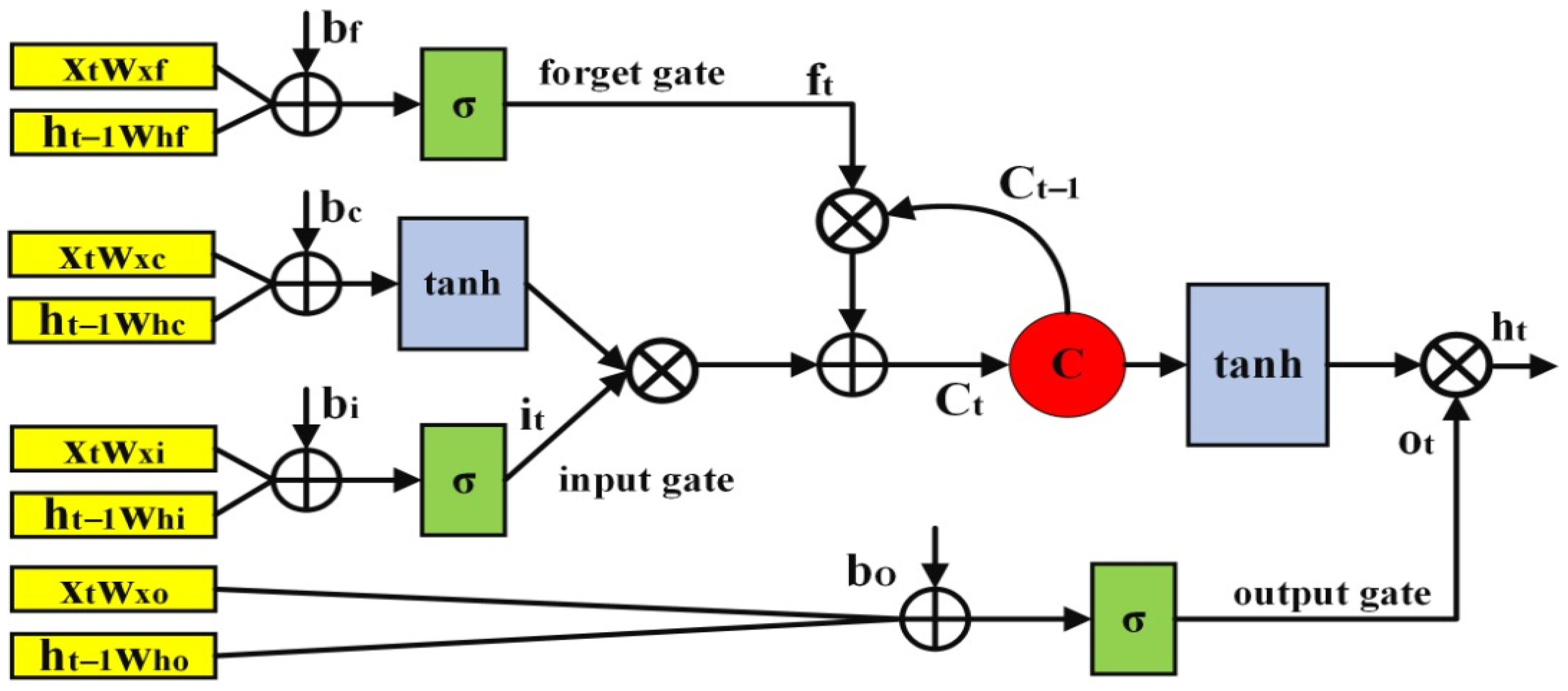
3.2. Long Short-Term Memory (LSTM)
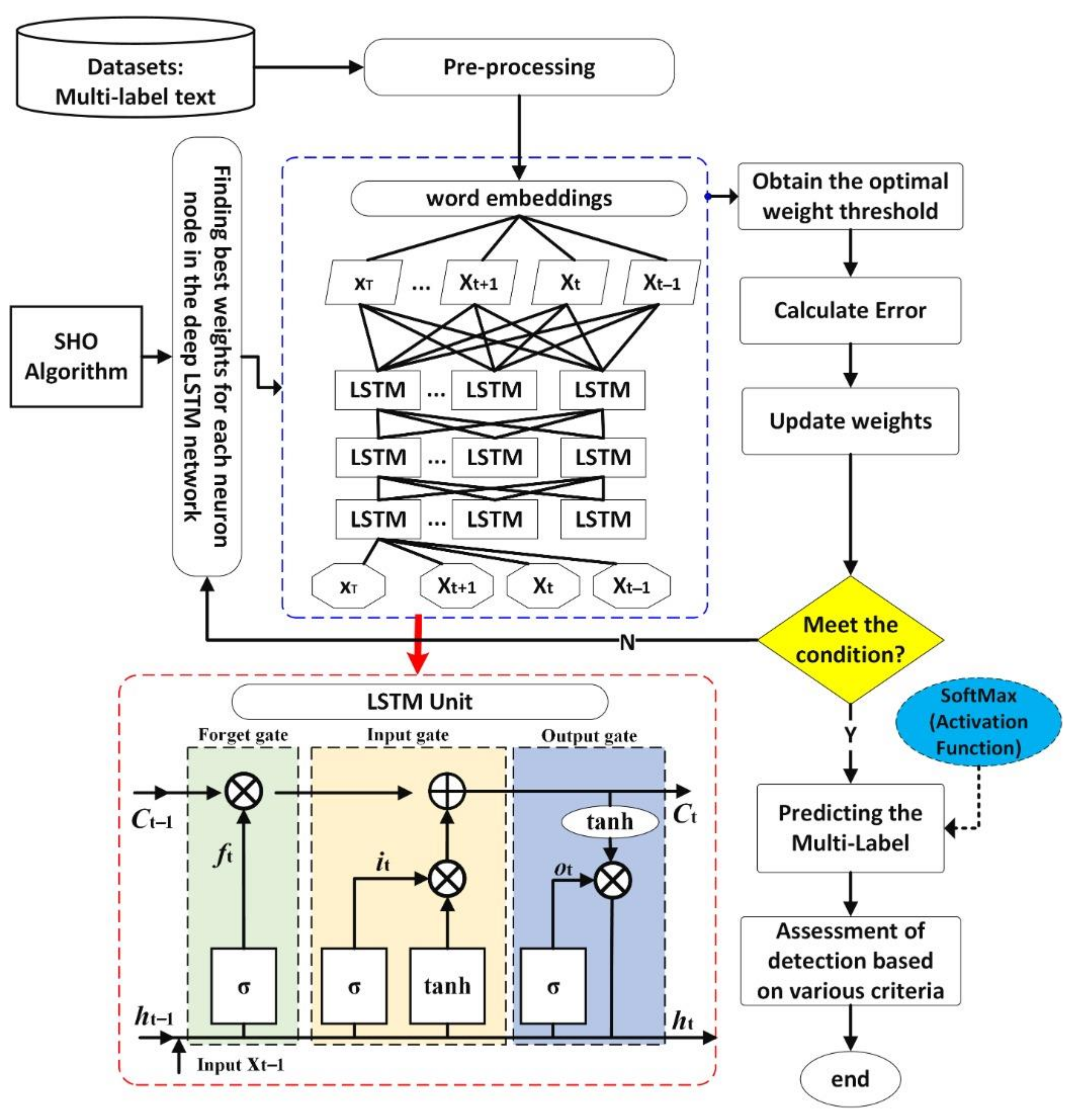
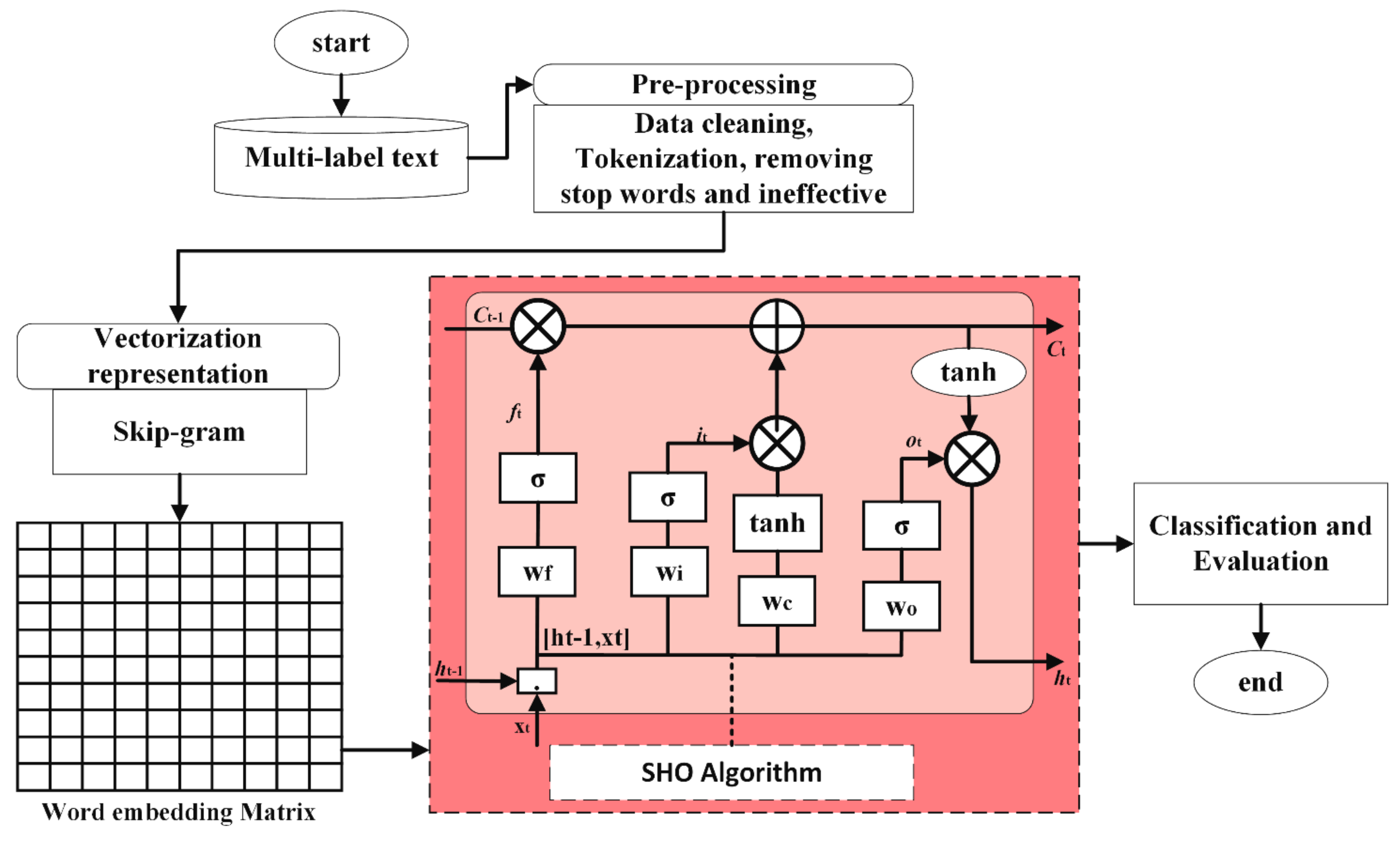
The LSTM is one of the most famous recursive neural networks that have had great success in various fields such as image processing, speech recognition, and emotion analysis. The LSTM has the advantages of non-linear predictability, fast convergence, and low complexity. Memory cell is the central part of LSTM, which consists of parameters and a single gateway system, and is used to make valuable or useless information. Figure 1 shows the structure of the LSTM cell.
There are three gates in each cell: the input gate, forget gate, and output gate. LSTM uses a separate memory to recall long-term dependencies, and then its update depends on the current input. At each time step, an LSTM takes the current input ( x t ) and the prior memory cell state ( c t 1 ) as input, and calculates the output ( o t ) and the current cell state ( c t ). In the defined equations, σ represents the sigmoid function ( σ X = 1 1 + e x ).
i t = σ i x t W x i + h t 1 W h i + b i
f t = σ f x t W x f + h t 1 W h f + b f
o t = σ o x t W x o + h t 1 W h o + b o
c t = f t c t 1 + i t t a n h x t W x c + h t 1 W h c + b c
h t = o t t a n h c t
where the variables are defined as: x t input vector, i t input gate activation vector, f t forget gate activation vector, o t output gate activation vector, h t hidden layer output vector, h t 1 R d h and d h hidden layer dimensions, and d input vector dimensions; c t is the cell state and c t 1 is the vector values of the memory unit in time t 1 . The parameters W and b are the weight matrix (input gate, forget gate, output, and cell mode) and bias.
Random initialization to LSTM connection weights causes the network to become stuck at local points, which affects the ability to learn non-linearly (i.e., predictive accuracy). To solve this problem, the SHO is used to optimize the initial weight of each node in the LSTM network.

4. Proposed Model

The proposed model is a combination of LSTM and SHO, where LSTM is a generalized example of the recursive neural network model. Unlike a conventional recursive neural network in which content is updated at every step, in an LSTM recursive neural network, the network can decide on the maintenance of current memory through gateways embedded in the network structure. LSTM is a recursive neural network architecture designed to store and access information better than the conventional recursive neural network version. The LSTM unit has one or more memory cells that are regulated by structures called the gate. Gates are a combination of sigmoid activation function and scalar multiplication function that is used to control information in the network. Figure 2 shows the steps of the proposed model.
The MLTC operation is generally divided by the proposed model according to Figure 3 into four main stages: pre-processing, word embedding, weight matrix by SHO, and LSTM-based classification.

4.1. Pre-Processing

Pre-processing is one of the main steps in MLTC. The most critical operations to be performed in the text pre-processing stage follow:
  • Convert numbers to words or delete numbers from textual data;
  • Clear punctuation marks, accent marks, and diagnostic marks;
  • Clear spaces from textual data;
  • In the rooting stage, the roots of the words are found, and the words are defined as a base;
  • Develop or expand abbreviations;
  • Delete ineffective words and particular words;
  • Synonymous words are eliminated and replaced by their more general meaning.

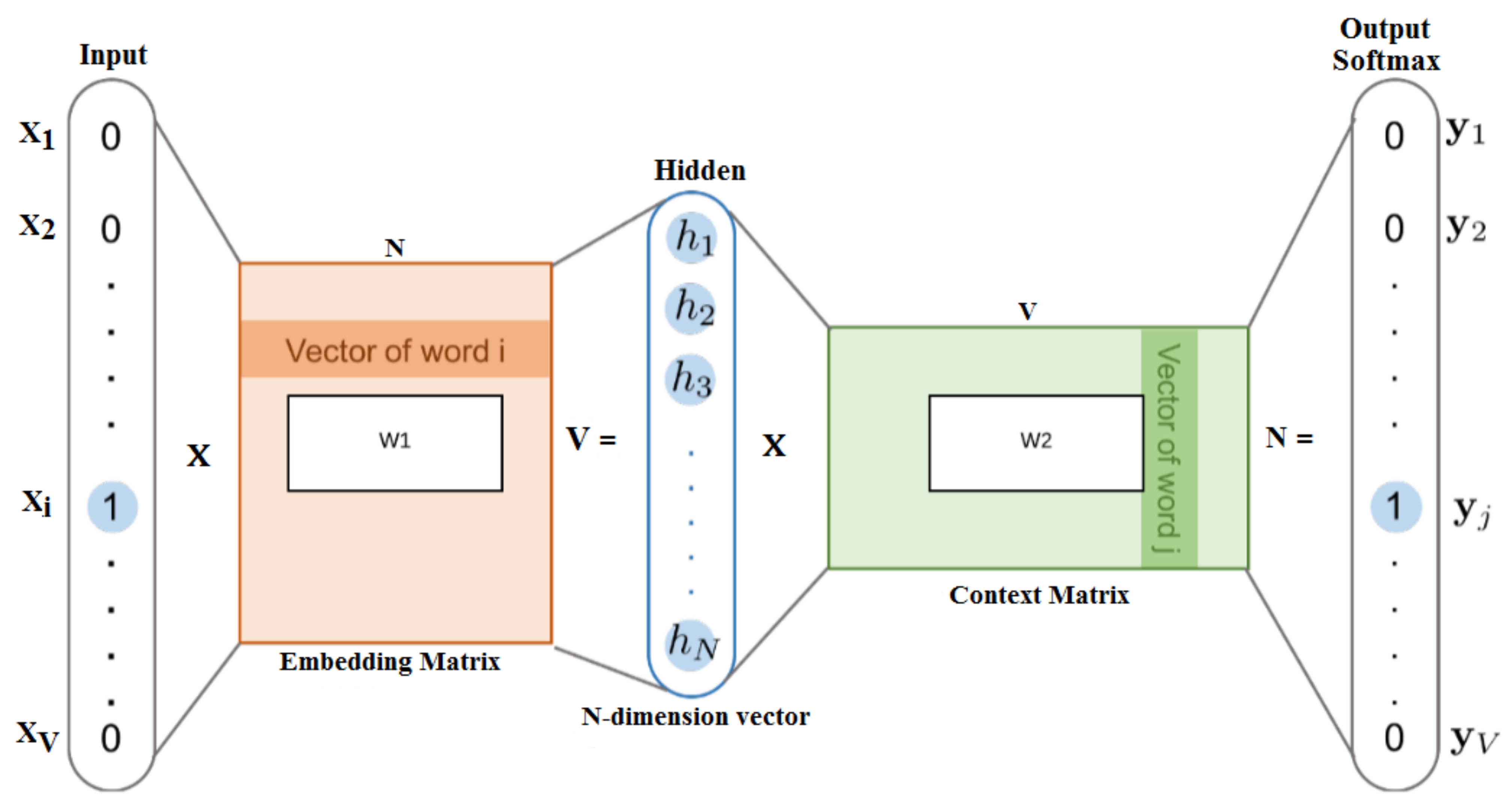
4.2. Embedding Words

The main task of word embedding in NLP is to display words in numerical vectors so that deep learning models can learn the hidden patterns in textual data. Word embedding helps to find attribute vectors to predict the following words. Word embedding n-dimensional vectors try to capture word meaning and content with their numerical values. The dataset is given to the skip-gram model to generate vectors. The model creates a vector for each vocabulary word, and then context properties are extracted from the vector documentation. In this paper, the skip-gram method [66] is used to predict context words (labels) using words called target words (input). Target words are considered input, and content words are considered output. Content words are words that are close or synonymous with the target words. Figure 4 shows the architecture of the skip-gram model.
The input vector (x) and the output vector (y) are coded based on the one-hot model. Some deep learning algorithms, such as the LSTM, use sequence order for better classification results. In this case, the one-hot method is used to extract documents based on digits 0 and 1. In this method, each dimension vector is assigned to one word in the dictionary, meaning that each dimension vector represents one word of the dictionary as shown in Table 1. Each word in specific dimensions of the vector x is equal to one, and the remaining dimensions of the vector are set to zero. The hidden layer (h) contains embedded words whose size is equal to N (N sizes of embedded word vectors for instruction). Additionally, V is the size of the dictionary (vectors are V-dimensions, and only one dimension has a value of 1, and the rest will be zero later). The purpose of skip-gram is to find output for content words using target words. Therefore L R d × V is a word embeddings matrix where d represents the vector dimensions of the words and V represents the number of words. In w i R d × 1 , the word i is equal to one row in the matrix L .
The conditional probability p r ( w i + j | w i ) is calculated by the skip-gram architecture using the given input word. The goal of skip-gram is to optimize the probability function for showing words in the output layer. In the skip-gram model, the maximum probability is defined according to Equation (17).
1 N i = 1 N k j i 0 l o g p r ( w i + j | w i )
where w 1 , w 2 , , w n are a sequence of training words and k is the window size of the training content. The tutorial’s goal is to minimize the total predictive error of all content words in the output layer. The principal probability p r ( w i + j | w i ) is defined using the s o f t m a x function according to Equation (18).
p r w i + j | w i = e x p M w i + j M w i L V e x p M w t M w i
M w and M w show w input and output, respectively, and V is the dictionary size.

4.3. SHO-LSTM

Many parameters must be controlled in the construction of the classification model by the LSTM, the most important of which is the weight of the neurons. To achieve better prediction results, the SHO is used to optimize the weight of neurons. The SHO can prevent the convergence of the network in the optimal local solution, and with a lower number of iterations, the LSTM can discover the optimal solutions. In the model training process, gates can memorize input vectors, forget previous records, and generate output vectors. In the proposed model, the input vector ( x t ) of length N is connected to the latent state variable (h) of length M, calculated at time t 1 . In particular, the forgetfulness gate layer (Equation (19)) decides what information should be removed from the cell state.
f t = σ w f 1 w f n T x t h t 1 + b f = σ w f 1 b f 1 T x t h t 1 1 w f M b f M T x t h t 1 1
f t k = σ w f k b f k T x t h t 1 1 ; k = 1 , 2 , , M
where w f k is the k th column of the vector w f and b f k is equal to the k th element of b f . The parameters c t and h t are defined according to Equations (21) and (22).
c t k = f t k . c t 1 k + i t k . t a n h w c . x t h t 1 + b c
h t k = o t k . t a n h c t k
The output matrix of the SHO-LSTM model’s hidden layer is parameter H, which is calculated according to Equation (23). According to Equation (23), the hidden layer consists of weights, bias, and input values.
H = [ w 1 , b 1 , x 1 w 2 , b 2 , x 1 w n , b n , x 1 w 1 , b 1 , x v w 2 , b 2 , x v w n , b n , x v ]
The hidden layer weights of the LSTM are included as the initial population value in the SHO. The LSTM weight size in the SHO-LSTM model is set in the range −1 and 1. The initial LSTM output error is used as the fit of the agents (hyenas), then the agents’ performance changes according to the conditions of the LSTM. Agents try to change and improve their position towards the best member of the population. The value of the agent’s position optimizer is utilized as the initial value of each weight of neuron in the LSTM to optimize the LSTM by the SHO. The position of the agents is constantly updated to reduce the network output layer error. In the proposed model, the fitness function of the agents is designed to evaluate the population factors. In the proposed model, the RMSE is designed according to Equation (24) as the LSTM output value and the actual value as a fitness function to measure the factors. The smaller the RMSE, the more logical the LSTM network weight settings for the agents, and the stronger the model’s generalizability. As N is the number of predictions, y ^ n is the predicted value of the model and y n is the actual value.
R M S E = 1 N n = 1 N y ^ n y n 2
Finally, the softmax layer is used to classify documents based on vectors according to Equation (25), where x i is the numeric value that appears in the output layer, and M represents the number of classes.
S o f t m a x   F u n c t i o n = σ x i = e x i k = 1 M e x k ; w h e r e   k = 1 , 2 , , M ,   a n d   x i ϵ R
This section describes the most critical evaluation criteria for MLTC [60]. Suppose m is the total number of samples in the test dataset; i represents an example in the test dataset. L is a set of labels L = λ j : j = 1 , , q , so that q is the total number of labels, and Z i and Y i refer to the predicted and real labels, respectively. Accuracy is one of the main criteria for evaluating MLTC.
A c c u r a c y = 1 m i = 1 m Z i Y i Z i Y i
P r e c i s i o n = 1 m i = 1 m Z i Y i Z i
R e c a l l = 1 m i = 1 m Z i Y i Y i
F M e a s u r e = 1 m i = 1 m 2 * Z i Y i Z i + Y i

5. Evaluation and Results

This section evaluates and describes the results of the proposed model that were obtained on different textual datasets. Anaconda software is a comprehensive Python programming environment that includes environments such as Jupiter Notebook for working with data. Four different datasets were used for evaluation according to Table 2. The evaluation was performed on a system with specifications of Core i7-4U, CPU@2.30 GHz, 6 GB RAM, and Windows 8.1 operating system. The datasets were divided into training sets and experimental sets, and 80% of the randomly selected texts were used for classification training and the remaining texts for the test phase.
To show the SHO-LSTM model’s efficiency, various meta-heuristic algorithms are used, such as Genetic Algorithm (GA) [67], Particle Swarm Optimization (PSO) [68], Artificial Bee Colony (ABC) [69], Harmony Algorithm Search (HAS) [70], and Differential Evolution (DE) [71]. The initial population and number of iterations in these algorithms are equal to SHO. The value of the parameters in meta-heuristic algorithms is set based on the base value.
Table 3 sets the initial value for the proposed model parameters. The definition and range of parameters is an essential factor after designing the proposed model. Usually, the value and range of parameters are obtained based on trial and error.
Table 4 shows the results of the SHO-LSTM model based on different criteria. As shown in Table 4, the accuracy of the SHO-LSTM model is higher than other models. The accuracy of the SHO-LSTM model in RCV1-v2 gained 87.65%, which has accuracy higher than LSTM. The PSO-LSTM model performed somewhat better than other models but has not reached the SHO-LSTM model.

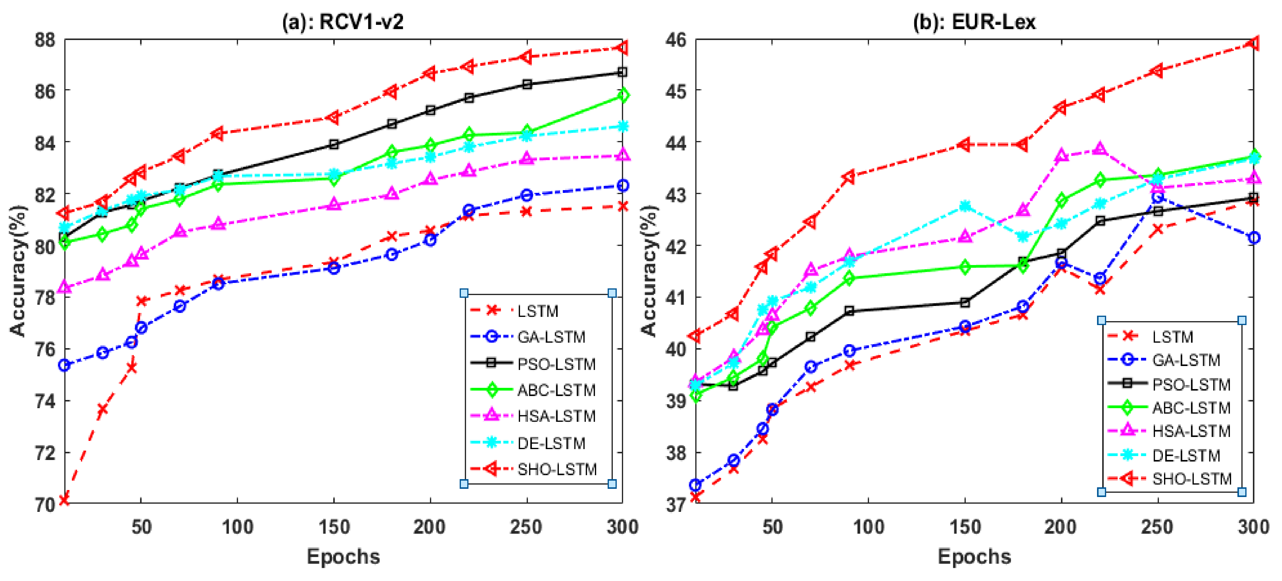
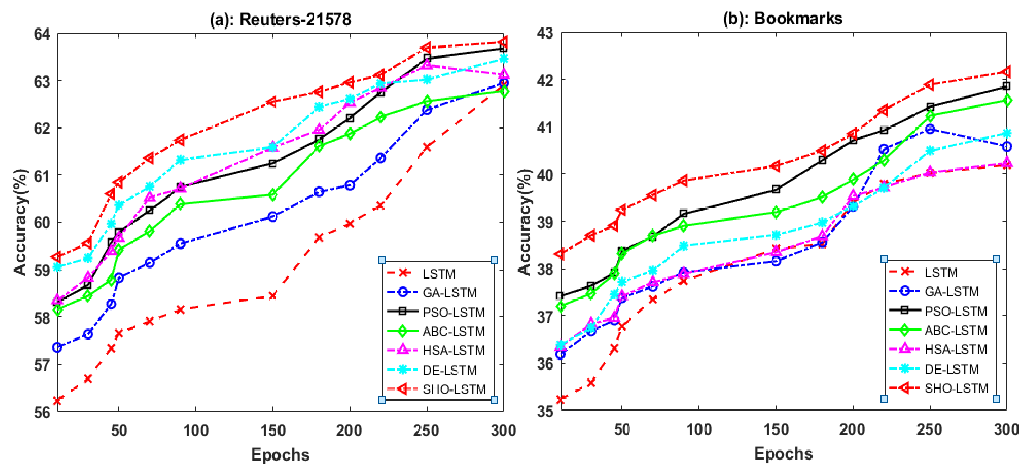
5.1. Evaluation Based on Epochs

In Figure 5, the results of the models are shown for RCV1-v2 and EUR-Lex with the epoch factor. Figure 5 shows that the SHO-LSTM model on RCV1-v2 has a higher accuracy percentage in the early stages, and its value starts with 81.25% and ends with 87.65%. It can be concluded that the convergence and achievement of the optimal solution in the SHO are better than the others. The GA-LSTM model has a lower percentage compared to the PSO, ABC, HSA, and DE models. The accuracy of the SHO-LSTM model on EUR-Lex in the early stages is 40.25% and 45.91%. Additionally, the percentage accuracy of PSO-LSTM and ABC-LSTM models is 42.92% and 43.72%, respectively. The SHO algorithm generates a set of values for the weights in each run, so the accuracy percentage varies. Furthermore, the weight matrix update in LSTM changes based on SHO, so this method causes the percentage of accuracy in the output to be different.
In Figure 6, the results of the models are shown for Reuters-21578 and Bookmarks with the epochs factor. The accuracy of the SHO-LSTM model on Reuters-21578 and Bookmarks are 63.81 and 42.16, respectively. The accuracy percentage of PSO-LSTM and ABC-LSTM on Reuters-21578 are 63.68 and 62.78, respectively. The accuracy percentage of PSO-LSTM and ABC-LSTM models on Bookmarks are 41.85 and 41.56, respectively. The accuracy of HSA-LSTM and DE-LSTM models on Reuters-21578 are 63.12 and 63.46, respectively. The accuracy of HSA-LSTM and DE-LSTM models on Bookmarks are 40.23 and 40.86, respectively.

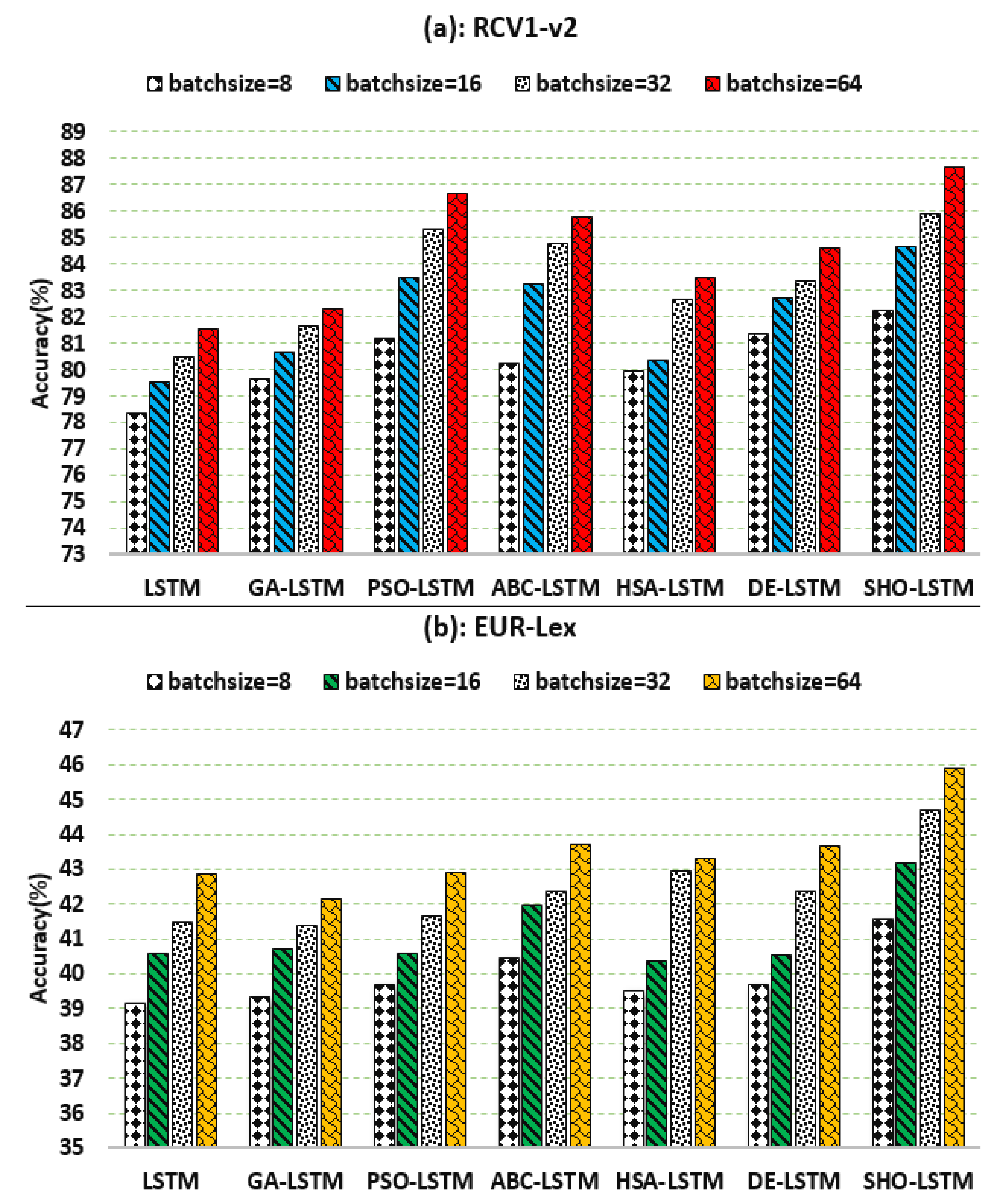
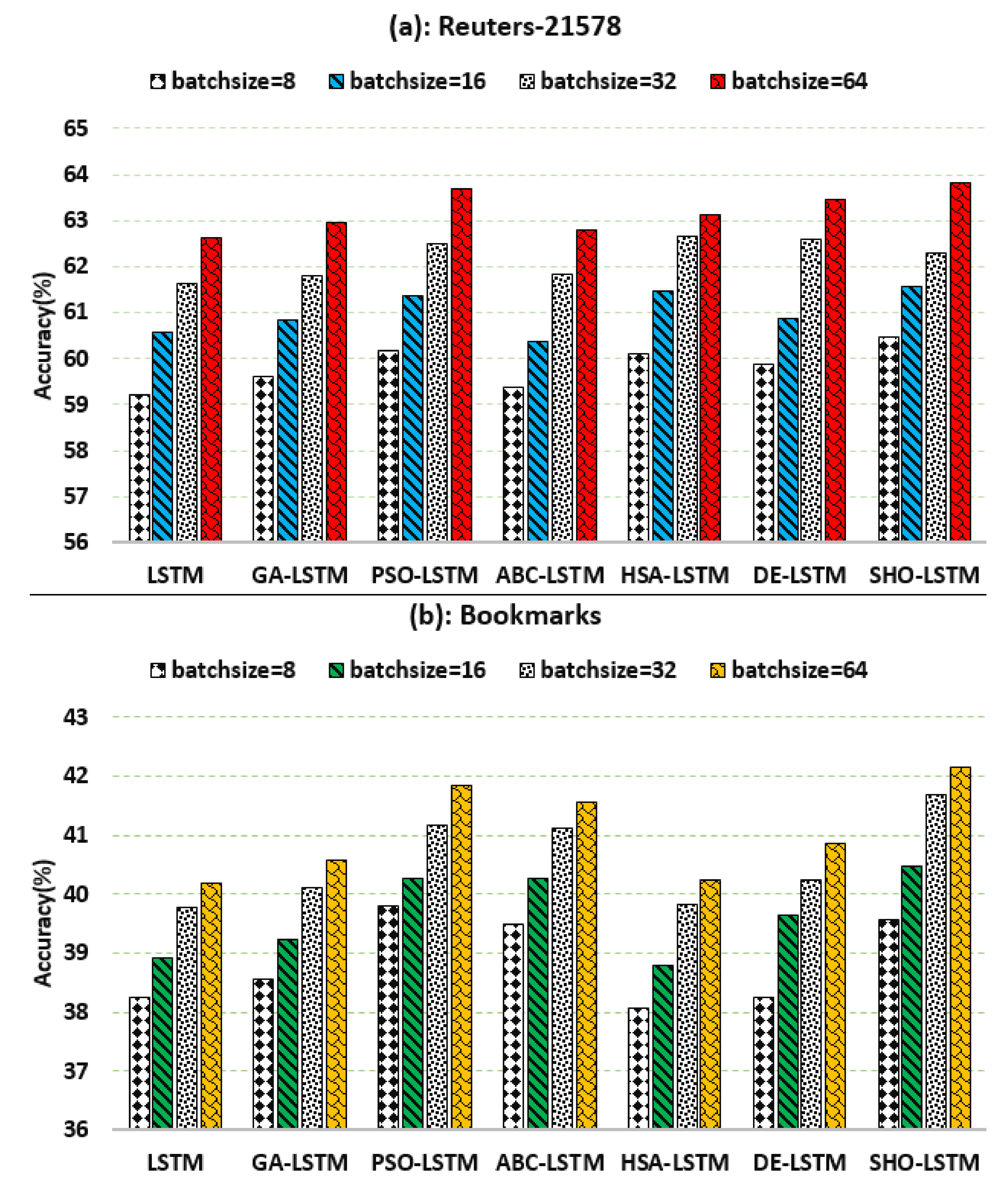
5.2. Evaluation based on Batchsize

In Figure 7a, the results of the models performed on four different datasets based on the batchsize factor are shown. As shown in Figure 7, the accuracy percentage of the SHO-LSTM model on RCV1-v2 for batchsize = 8, batchsize = 16, batchsize = 32, and batchsize = 34 is 82.25, 84.67, 85.92, and 87.65, respectively. The accuracy percentage of SHO-LSTM model on EUR-Lex for batchsize = 8, batchsize = 16, batchsize = 32, and batchsize = 34 is equal to 41.56, 43.18, 44.68, and 45.91, respectively. The accuracy of the SHO-LSTM model on Reuters-21578 for batchsize = 8, batchsize = 16, batchsize = 32, and batchsize = 34 is 60.48, 61.56, 62.29, and 63.81, respectively. The accuracy of the SHO-LSTM model on Bookmarks for batchsize = 8, batchsize = 16, batchsize = 32, and batchsize = 34 is equal to 39.56, 40.48, 41.68, and 42.16, respectively.
According to Figure 7b, the accuracy percentage of PSO-LSTM and ABC-LSTM on RCV1-v2 for batchsize = 8 is 81.16 and 80.24, respectively. The percentages of PSO-LSTM and ABC-LSTM on EUR-Lex for batchsize = 8 are 39.67 and 40.46, respectively. The accuracy percentage of PSO-LSTM and ABC-LSTM on Reuters-21578 for batchsize = 8 is 60.17 and 59.38, respectively. The accuracy of PSO-LSTM and ABC-LSTM on Bookmarks for batchsize = 8 is 39.79% and 39.48%, respectively.
Figure 7a shows that the accuracy percentage of GA-LSTM and PSO-LSTM models on RCV1-v2 for batch size = 32 is 81.67 and 85.31, respectively. The accuracy percentage of ABC-LSTM, HSA-LSTM, and DE-LSTM models on RCV1-v2 for batch size = 32 is 84.76, 82.66, and 83.34, respectively. The accuracy percentage of GA-LSTM and PSO-LSTM models on RCV1-v2 for batch size = 64 is 82.32 and 86.69, respectively. The accuracy percentage of ABC-LSTM, HSA-LSTM, and DE-LSTM models on RCV1-v2 for batch size = 64 is 85.79, 83.47, and 84.61, respectively. The accuracy percentage of SHO-LSTM on RCV1-v2 for batch size = 32 and batch size = 64 is 85.92 and 87.65, respectively. The results based on batch size showed that the SHO-LSTM model has a higher percentage in comparison with other models.
Figure 7b shows that the accuracy percentage of GA-LSTM and PSO-LSTM models on EUR-Lex for batchsize = 32 is 41.38 and 41.67, respectively. The accuracy percentage of ABC-LSTM, HSA-LSTM, and DE-LSTM models on EUR-Lex for batchsize = 32 is 42.38, 42.94, and 42.38, respectively. The accuracy percentage of GA-LSTM and PSO-LSTM models on EUR-Lex for batchsize = 64 is 42.15 and 42.92, respectively. The accuracy percentage of ABC-LSTM, HSA-LSTM, and DE-LSTM models on EUR-Lex for batchsize = 64 is 43.72, 43.29, and 43.38, respectively. The accuracy percentage of SHO-LSTM on EUR-Lex for batchsize = 32 and batchsize = 64 is 44.68 and 45.91, respectively.
Figure 8a shows that the accuracy percentage of GA-LSTM and PSO-LSTM models on Reuters-21578 for batchsize = 32 is 61.81 and 62.51, respectively. The accuracy percentage of ABC-LSTM, HSA-LSTM, and DE-LSTM models on Reuters-21578 for batchsize = 32 is 61.84, 62.66, and 62.59, respectively. The accuracy percentage of GA-LSTM and PSO-LSTM models on Reuters-21578 for batchsize = 64 is 62.95 and 63.68, respectively. The accuracy percentage of ABC-LSTM, HSA-LSTM, and DE-LSTM models on Reuters-21578 for batchsize = 64 is 62.78, 63.12, and 63.46, respectively. The accuracy percentage of SHO-LSTM on Reuters-21578 for batchsize = 32 and batchsize = 64 is 62.29 and 63.81, respectively.
Figure 8b shows that the accuracy percentage of GA-LSTM and PSO-LSTM models on Bookmarks for batchsize = 32 is 40.12 and 41.17, respectively. The accuracy percentage of ABC-LSTM, HSA-LSTM and DE-LSTM models on Bookmarks for batchsize = 32 is 41.12, 39.84, and 40.24, respectively. The accuracy percentage of GA-LSTM and PSO-LSTM models on Bookmarks for batchsize = 64 is 40.58 and 41.85, respectively. The accuracy percentage of ABC-LSTM, HSA-LSTM and DE-LSTM models on Bookmarks for batchsize = 64 is 41.56, 40.23, and 40.86, respectively. The accuracy percentage of SHO-LSTM on Bookmarks for batchsize = 32 and batchsize = 64 is 41.68 and 42.16, respectively.

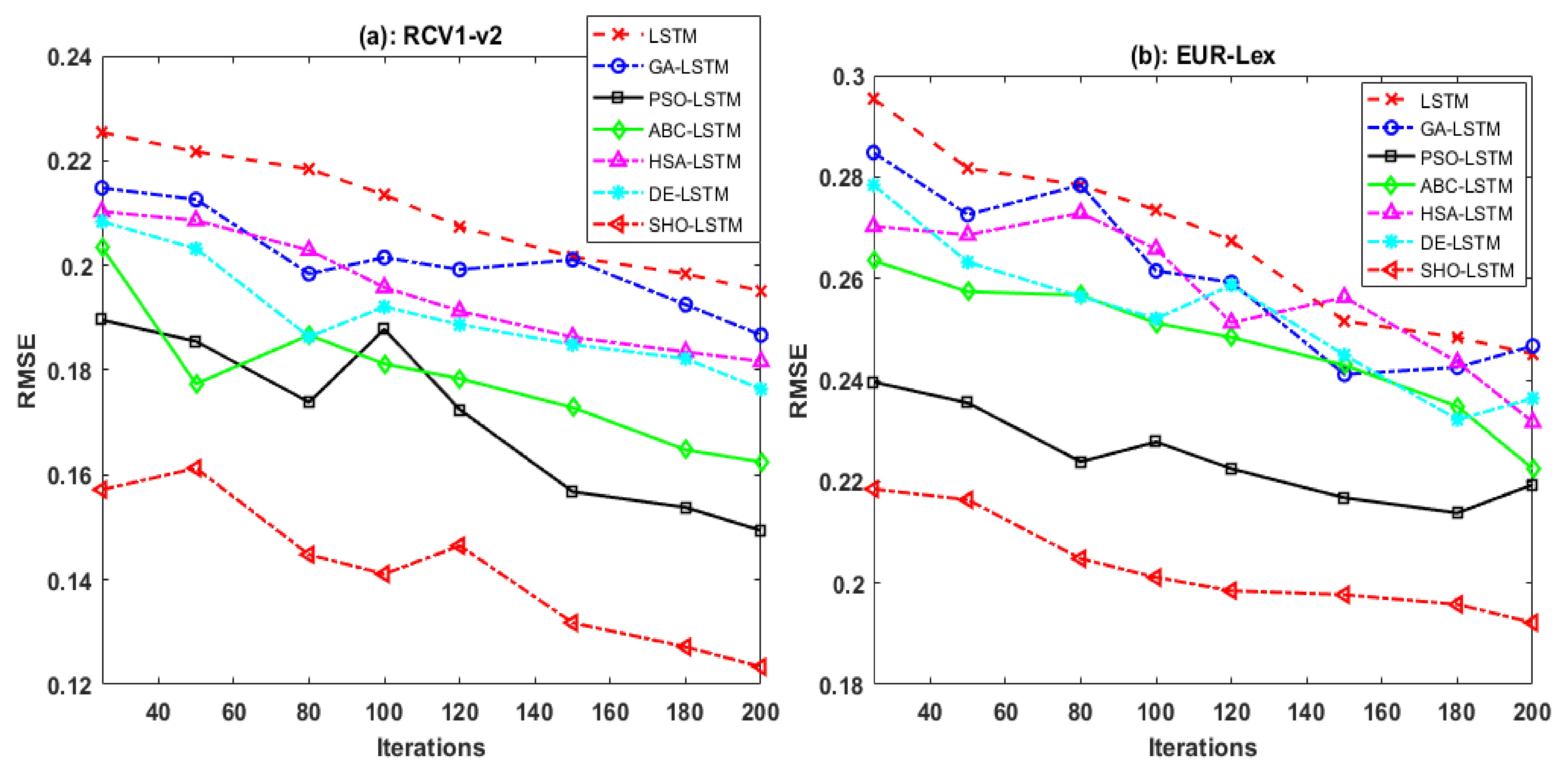
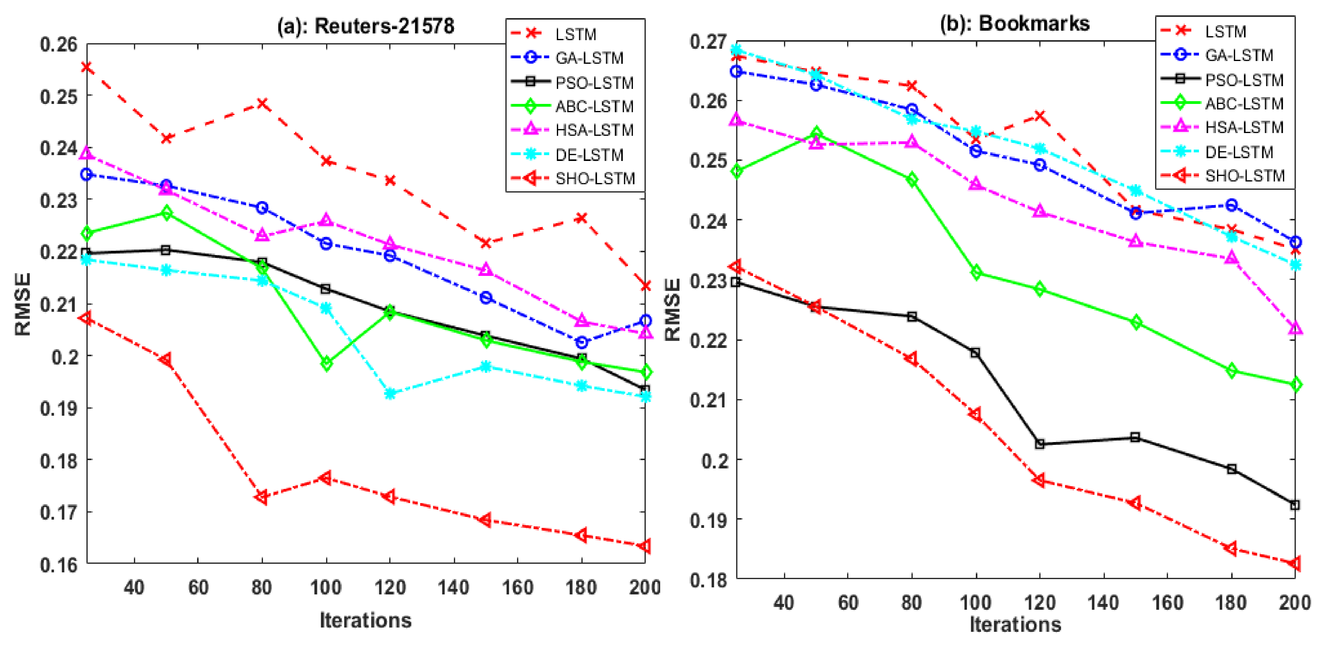
5.3. Evaluation Based on the Number of Iterations

Figure 9 evaluates the models based on the number of iterations and RMSE. Figure 9 shows that the SHO-LSTM model on the RCV1-v2 has a lower RMSE compared to other models and its value is equal to 0.1234 in 200 iterations. The RMSE values for PSO-LSTM and ABC-LSTM are 0.1494 and 0.1625, respectively. The RMSE value in the SHO-LSTM model on EUR-Lex for 200 iterations is 0.1922. The RMSE values for PSO-LSTM and ABC-LSTM are 0.2194 and 0.2225, respectively. The RMSE values for the GA-LSTM and DE-LSTM models are 0.2467 and 0.2364, respectively.
Figure 10 shows that the SHO-LSTM model on the Reuters-21578 has a lower RMSE value compared to other models, and its value for 200 iterations is equal to 0.1634. The RMSE values for PSO-LSTM and ABC-LSTM are 0.1934 and 0.1968, respectively. The RMSE value in the SHO-LSTM model on Bookmarks for 200 iterations is 0.1826. The RMSE values for PSO-LSTM and ABC-LSTM are 0.1924 and 0.2125, respectively. The RMSE values for the GA-LSTM and DE-LSTM models are 0.2363 and 0.2325, respectively.
According to the results, the SHO-LSTM model had higher detection accuracy and better performance in MLTC compared to other models. The SHO was able to increase the LSTM performance in text recognition and reduce the amount of error. On the other hand, the number of epochs was also influential in the accuracy of diagnosis and based on various experiments. It was proven that if the number of epochs is equal to 300, then the best accuracy of diagnosis is obtained. The SHO-LSTM had better classification effects on RCV1-v2. In addition, we found that most of the models listed in Table 4 performed well on Reuters-21578.

5.4. Comparison and Evaluation

In this section, the SHO-LSTM model is compared with other models. The results of comparisons show that the accuracy percentage of the SHO-LSTM model is higher than other models. The accuracy percentages of DSRM-DNN-1 and DSRM-DNN-2 on RCV1-v2 are 0.8164 and 0.8326, respectively. Additionally, the accuracy percentage of the SHO-LSTM model is 0.8974 on RCV1-v2. The accuracy percentage of DSRM-DNN-1 and DSRM-DNN-2 on EUR-Lex is 0.4298 and 0.4315, respectively, while the accuracy percentage of the SHO-LSTM model is 0.4633. The accuracy percentage of DSRM-DNN-1 and DSRM-DNN-2 on Reuters-21578 is 0.4913 and 0.6147, respectively, while the accuracy percentage of the SHO-LSTM model is 0.6427. The accuracy percentages of DSRM-DNN-1 and DSRM-DNN-2 on Bookmarks are 0.3841 and 0.4018, respectively, while the accuracy percentage of the proposed model is 0.4251.
According to the results of Table 5, the accuracy percentages of ML-Reasoner, ML-Reasoner-LSTM, and ML-Reasoner-BERT on RCV1-v2 are 0.9120, 0.8970, and 0.8900, respectively. The accuracy percentages of H-AGCRNN, HAGTP-GCN, and HCSM on RCV1-v2 are 0.7960, 0.8710, and 08940, respectively.
The results show that SHO is superior to other models. Studies have shown that SHO has the following benefits [65]: fast convergence rate and balance between exploration and exploitation. Furthermore, the efficiency and power of SHO have already been proven [72]. Therefore, in this paper, SHO is used to improve LSTM.

6. Conclusions and Future Works

In this paper, after a thorough review of previous studies on the operation of LSTM with meta-heuristic algorithms, a new model based on LSTM and SHO for MLTC was proposed. Deep learning algorithms can be an excellent way to increase detection accuracy due to their valuable achievements in the MLTC problem. In the SHO-LSTM model, the SHO was used to optimize the LSTM weight matrix. The SHO-LSTM model was tested and evaluated on four different datasets of texts. The results showed that the accuracy of the SHO-LSTM model on RCV1-v2, EUR-Lex, Reuters-21578, and Bookmarks were 87.65, 45.91, 63.81, and 42.16, respectively. The results showed that the accuracy of the SHO-LSTM model on RCV1-v2 improved by about 7.52% compared to LSTM. Additionally, the SHO-LSTM model significantly reduced the RMSE value compared to other models, indicating that the SHO has good convergence capability in finding the optimal solution. Comparisons showed that the PSO-LSTM and ABC-LSTM models had better detection accuracy compared to LSTM and GA-LSTM. Future work proposed will combine machine learning algorithms with CNN and RNN networks to optimize parameters (number of layers, number of neurons, window size) to solve various problems such as classification and clustering.

Author Contributions

Conceptualization, H.K.M. and F.S.G.; methodology, H.K.M.; software, H.K.M. and F.S.G.; validation, F.S.G., K.M., and A.B.S.; formal analysis, H.K.M.; investigation, F.S.G.; resources, H.K.M.; data curation, F.S.G.; writing—original draft preparation, H.K.M.; writing—review and editing, F.S.G.; visualization, K.M.; supervision, F.S.G.; project administration, F.S.G. All authors have read and agreed to the published version of the manuscript.

Funding

This research received no external funding.

Conflicts of Interest

The authors declare no conflict of interest.

References

  1. Feremans, L.; Cule, B.; Vens, C.; Goethals, B. Combining instance and feature neighbours for extreme multi-label classification. Int. J. Data Sci. Anal. 2020, 10, 215–231. [Google Scholar] [CrossRef]
  2. Rubin, T.N.; Chambers, A.; Smyth, P.; Steyvers, M. Statistical topic models for multi-label document classification. Mach. Learn. 2012, 88, 157–208. [Google Scholar] [CrossRef] [Green Version]
  3. Liu, N.; Wang, Q.; Ren, J. Label-Embedding Bi-directional Attentive Model for Multi-label Text Classification. Neural Process. Lett. 2021, 53, 375–389. [Google Scholar] [CrossRef]
  4. Gharehchopogh, F.S.; Khalifelu, Z.A. Analysis and evaluation of unstructured data: Text mining versus natural language processing. In Proceedings of the 2011 5th International Conference on Application of Information and Communication Technologies (AICT), Baku, Azerbaijan, 12–14 October 2011; pp. 1–4. [Google Scholar]
  5. Mittal, V.; Gangodkar, D.; Pant, B. Deep Graph-Long Short-Term Memory: A Deep Learning Based Approach for Text Classification. Wirel. Pers. Commun. 2021, 119, 2287–2301. [Google Scholar] [CrossRef]
  6. Liao, W.; Wang, Y.; Yin, Y.; Zhang, X.; Ma, P. Improved sequence generation model for multi-label classification via CNN and initialized fully connection. Neurocomputing 2020, 382, 188–195. [Google Scholar] [CrossRef]
  7. Liu, G.; Guo, J. Bidirectional LSTM with attention mechanism and convolutional layer for text classification. Neurocomputing 2019, 337, 325–338. [Google Scholar] [CrossRef]
  8. Zhan, H.; Lyu, S.; Lu, Y.; Pal, U. DenseNet-CTC: An end-to-end RNN-free architecture for context-free string recognition. Comput. Vis. Image Underst. 2021, 204, 103168. [Google Scholar] [CrossRef]
  9. Fasihi, M.; Nadimi-Shahraki, M.H.; Jannesari, A. A Shallow 1-D Convolution Neural Network for Fetal State Assessment Based on Cardiotocogram. SN Comput. Sci. 2021, 2, 287. [Google Scholar] [CrossRef]
  10. Fasihi, M.; Nadimi-Shahraki, M.H.; Jannesari, A. Multi-Class Cardiovascular Diseases Diagnosis from Electrocardiogram Signals using 1-D Convolution Neural Network. In Proceedings of the 2020 IEEE 21st International Conference on Information Reuse and Integration for Data Science (IRI), Las Vegas, NV, USA, 11–13 August 2020; pp. 372–378. [Google Scholar]
  11. Lee, T. EMD and LSTM Hybrid Deep Learning Model for Predicting Sunspot Number Time Series with a Cyclic Pattern. Sol. Phys. 2020, 295, 82. [Google Scholar] [CrossRef]
  12. Hochreiter, S.; Schmidhuber, J. Long Short-Term Memory. Neural Comput. 1997, 9, 1735–1780. [Google Scholar] [CrossRef] [PubMed]
  13. Jain, G.; Sharma, M.; Agarwal, B. Optimizing semantic LSTM for spam detection. Int. J. Inf. Technol. 2019, 11, 239–250. [Google Scholar] [CrossRef]
  14. Alotaibi, F.M.; Asghar, M.Z.; Ahmad, S. A Hybrid CNN-LSTM Model for Psychopathic Class Detection from Tweeter Users. Cogn. Comput. 2021, 13, 709–723. [Google Scholar] [CrossRef]
  15. Wang, R.; Peng, C.; Gao, J.; Gao, Z.; Jiang, H. A dilated convolution network-based LSTM model for multi-step prediction of chaotic time series. Comput. Appl. Math. 2019, 39, 30. [Google Scholar] [CrossRef]
  16. Yang, Z.; Wei, C. Prediction of equipment performance index based on improved chaotic lion swarm optimization–LSTM. Soft Comput. 2020, 24, 9441–9465. [Google Scholar] [CrossRef]
  17. Yuan, X.; Chen, C.; Lei, X.; Yuan, Y.; Muhammad Adnan, R. Monthly runoff forecasting based on LSTM–ALO model. Stoch. Environ. Res. Risk Assess. 2018, 32, 2199–2212. [Google Scholar] [CrossRef]
  18. Li, S.; You, X.; Liu, S. Multiple ant colony optimization using both novel LSTM network and adaptive Tanimoto communication strategy. Appl. Intell. 2021, 51, 5644–5664. [Google Scholar] [CrossRef]
  19. Gong, C.; Wang, X.; Gani, A.; Qi, H. Enhanced long short-term memory with fireworks algorithm and mutation operator. J. Supercomput. 2021, 77, 12630–12646. [Google Scholar] [CrossRef]
  20. Goluguri, N.V.R.R.; Devi, K.S.; Srinivasan, P. Rice-net: An efficient artificial fish swarm optimization applied deep convolutional neural network model for identifying the Oryza sativa diseases. Neural Comput. Appl. 2020, 33, 5869–5884. [Google Scholar] [CrossRef]
  21. Jalali, S.M.J.; Ahmadian, S.; Khodayar, M.; Khosravi, A.; Ghasemi, V.; Shafie-khah, M.; Nahavandi, S.; Catalão, J.P.S. Towards novel deep neuroevolution models: Chaotic levy grasshopper optimization for short-term wind speed forecasting. Eng. Comput. 2021. [Google Scholar] [CrossRef]
  22. Ghulanavar, R.; Dama, K.K.; Jagadeesh, A. Diagnosis of faulty gears by modified AlexNet and improved grasshopper optimization algorithm (IGOA). J. Mech. Sci. Technol. 2020, 34, 4173–4182. [Google Scholar] [CrossRef]
  23. Zhang, Y.; Li, R.; Zhang, J. Optimization scheme of wind energy prediction based on artificial intelligence. Environ. Sci. Pollut. Res. 2021, 28, 39966–39981. [Google Scholar] [CrossRef] [PubMed]
  24. Rajeev, R.; Samath, J.A.; Karthikeyan, N.K. An Intelligent Recurrent Neural Network with Long Short-Term Memory (LSTM) BASED Batch Normalization for Medical Image Denoising. J. Med. Syst. 2019, 43, 234. [Google Scholar] [CrossRef] [PubMed]
  25. Vijayaprabakaran, K.; Sathiyamurthy, K. Neuroevolution based hierarchical activation function for long short-term model network. J. Ambient Intell. Humaniz. Comput. 2021, 12, 10757–10768. [Google Scholar] [CrossRef]
  26. Sikkandar, H.; Thiyagarajan, R. Deep learning based facial expression recognition using improved Cat Swarm Optimization. J. Ambient Intell. Humaniz. Comput. 2021, 12, 3037–3053. [Google Scholar] [CrossRef]
  27. Lan, K.; Liu, L.; Li, T.; Chen, Y.; Fong, S.; Marques, J.A.L.; Wong, R.K.; Tang, R. Multi-view convolutional neural network with leader and long-tail particle swarm optimizer for enhancing heart disease and breast cancer detection. Neural Comput. Appl. 2020, 32, 15469–15488. [Google Scholar] [CrossRef]
  28. Nandhini, S.; Ashokkumar, K. Improved crossover based monarch butterfly optimization for tomato leaf disease classification using convolutional neural network. Multimed. Tools Appl. 2021, 80, 18583–18610. [Google Scholar] [CrossRef]
  29. Dhiman, G.; Kumar, V. Spotted hyena optimizer: A novel bio-inspired based metaheuristic technique for engineering applications. Adv. Eng. Softw. 2017, 114, 48–70. [Google Scholar] [CrossRef]
  30. Wang, R.; Ridley, R.; Su, X.; Qu, W.; Dai, X. A novel reasoning mechanism for multi-label text classification. Inf. Process. Manag. 2021, 58, 102441. [Google Scholar] [CrossRef]
  31. Omar, A.; Mahmoud, T.M.; Abd-El-Hafeez, T.; Mahfouz, A. Multi-label Arabic text classification in Online Social Networks. Inf. Syst. 2021, 100, 101785. [Google Scholar] [CrossRef]
  32. Udandarao, V.; Agarwal, A.; Gupta, A.; Chakraborty, T. InPHYNet: Leveraging attention-based multitask recurrent networks for multi-label physics text classification. Knowl.-Based Syst. 2021, 211, 106487. [Google Scholar] [CrossRef]
  33. Ciarelli, P.M.; Oliveira, E.; Salles, E.O.T. Multi-label incremental learning applied to web page categorization. Neural Comput. Appl. 2014, 24, 1403–1419. [Google Scholar] [CrossRef]
  34. Yao, L.; Sheng, Q.Z.; Ngu, A.H.H.; Gao, B.J.; Li, X.; Wang, S. Multi-label classification via learning a unified object-label graph with sparse representation. World Wide Web. 2016, 19, 1125–1149. [Google Scholar] [CrossRef]
  35. Ghiandoni, G.M.; Bodkin, M.J.; Chen, B.; Hristozov, D.; Wallace, J.E.A.; Webster, J.; Gillet, V.J. Enhancing reaction-based de novo design using a multi-label reaction class recommender. J. Comput.-Aided Mol. Des. 2020, 34, 783–803. [Google Scholar] [CrossRef] [PubMed] [Green Version]
  36. Laghmari, K.; Marsala, C.; Ramdani, M. An adapted incremental graded multi-label classification model for recommendation systems. Prog. Artif. Intell. 2018, 7, 15–29. [Google Scholar] [CrossRef]
  37. Zou, Y.-p.; Ouyang, J.-h.; Li, X.-m. Supervised topic models with weighted words: Multi-label document classification. Front. Inf. Technol. Electron. Eng. 2018, 19, 513–523. [Google Scholar] [CrossRef]
  38. Li, X.; Ouyang, J.; Zhou, X. Labelset topic model for multi-label document classification. J. Intell. Inf. Syst. 2016, 46, 83–97. [Google Scholar] [CrossRef]
  39. Wang, B.; Hu, X.; Li, P.; Yu, P.S. Cognitive structure learning model for hierarchical multi-label text classification. Knowl.-Based Syst. 2021, 218, 106876. [Google Scholar] [CrossRef]
  40. Neshat, M.; Nezhad, M.M.; Abbasnejad, E.; Mirjalili, S.; Tjernberg, L.B.; Astiaso Garcia, D.; Alexander, B.; Wagner, M. A deep learning-based evolutionary model for short-term wind speed forecasting: A case study of the Lillgrund offshore wind farm. Energy Convers. Manag. 2021, 236, 114002. [Google Scholar] [CrossRef]
  41. Kwon, D.-H.; Kim, J.-B.; Heo, J.-S.; Kim, C.-M.; Han, Y.-H. Time Series Classification of Cryptocurrency Price Trend Based on a Recurrent LSTM Neural Network. J. Inf. Process. Syst. 2019, 15, 694–706. [Google Scholar]
  42. Koutsoukas, A.; Monaghan, K.J.; Li, X.; Huan, J. Deep-learning: Investigating deep neural networks hyper-parameters and comparison of performance to shallow methods for modeling bioactivity data. J. Cheminform. 2017, 9, 42. [Google Scholar] [CrossRef] [PubMed]
  43. Pareek, V.; Chaudhury, S. Deep learning-based gas identification and quantification with auto-tuning of hyper-parameters. Soft Comput. 2021, 25, 14155–14170. [Google Scholar] [CrossRef]
  44. Ibrahim, M.A.; Ghani Khan, M.U.; Mehmood, F.; Asim, M.N.; Mahmood, W. GHS-NET a generic hybridized shallow neural network for multi-label biomedical text classification. J. Biomed. Inform. 2021, 116, 103699. [Google Scholar] [CrossRef] [PubMed]
  45. Duan, X.; Ying, S.; Cheng, H.; Yuan, W.; Yin, X. OILog: An online incremental log keyword extraction approach based on MDP-LSTM neural network. Inf. Syst. 2021, 95, 101618. [Google Scholar] [CrossRef]
  46. Song, X.; Liu, Y.; Xue, L.; Wang, J.; Zhang, J.; Wang, J.; Jiang, L.; Cheng, Z. Time-series well performance prediction based on Long Short-Term Memory (LSTM) neural network model. J. Pet. Sci. Eng. 2020, 186, 106682. [Google Scholar] [CrossRef]
  47. Das Chakladar, D.; Dey, S.; Roy, P.P.; Dogra, D.P. EEG-based mental workload estimation using deep BLSTM-LSTM network and evolutionary algorithm. Biomed. Signal Process. Control 2020, 60, 101989. [Google Scholar] [CrossRef]
  48. Shahid, F.; Zameer, A.; Muneeb, M. A novel genetic LSTM model for wind power forecast. Energy 2021, 223, 120069. [Google Scholar] [CrossRef]
  49. Memarzadeh, G.; Keynia, F. A new short-term wind speed forecasting method based on fine-tuned LSTM neural network and optimal input sets. Energy Convers. Manag. 2020, 213, 112824. [Google Scholar] [CrossRef]
  50. Ding, N.; Li, H.; Yin, Z.; Zhong, N.; Zhang, L. Journal bearing seizure degradation assessment and remaining useful life prediction based on long short-term memory neural network. Measurement 2020, 166, 108215. [Google Scholar] [CrossRef]
  51. Huang, Y.-F.; Chen, P.-H. Fake news detection using an ensemble learning model based on Self-Adaptive Harmony Search algorithms. Expert Syst. Appl. 2020, 159, 113584. [Google Scholar] [CrossRef]
  52. Prasanth, S.; Singh, U.; Kumar, A.; Tikkiwal, V.A.; Chong, P.H.J. Forecasting spread of COVID-19 using google trends: A hybrid GWO-deep learning approach. Chaos Solitons Fractals 2021, 142, 110336. [Google Scholar] [CrossRef]
  53. Liang, J.; Yang, H.; Gao, J.; Yue, C.; Ge, S.; Qu, B. MOPSO-Based CNN for Keyword Selection on Google Ads. IEEE Access 2019, 7, 125387–125400. [Google Scholar] [CrossRef]
  54. Gadekallu, T.R.; Alazab, M.; Kaluri, R.; Maddikunta, P.K.R.; Bhattacharya, S.; Lakshmanna, K.; Parimala, M. Hand gesture classification using a novel CNN-crow search algorithm. Complex Intell. Syst. 2021, 7, 1855–1868. [Google Scholar] [CrossRef]
  55. Kumar, K.; Haider, M.T.U. Enhanced Prediction of Intra-day Stock Market Using Metaheuristic Optimization on RNN–LSTM Network. New Gener. Comput. 2021, 39, 231–272. [Google Scholar] [CrossRef]
  56. Gundu, V.; Simon, S.P. PSO–LSTM for short term forecast of heterogeneous time series electricity price signals. J. Ambient Intell. Humaniz. Comput. 2021, 12, 2375–2385. [Google Scholar] [CrossRef]
  57. Peng, L.; Zhu, Q.; Lv, S.-X.; Wang, L. Effective long short-term memory with fruit fly optimization algorithm for time series forecasting. Soft Comput. 2020, 24, 15059–15079. [Google Scholar] [CrossRef]
  58. Rashid, N.A.; Abdul Aziz, I.; Hasan, M.H.B. Machine Failure Prediction Technique Using Recurrent Neural Network Long Short-Term Memory-Particle Swarm Optimization Algorithm. In Artificial Intelligence Methods in Intelligent Algorithms; Springer: Cham, Switzerland, 2019; pp. 243–252. [Google Scholar]
  59. Singh, P.; Sehgal, P. G.V Black dental caries classification and preparation technique using optimal CNN-LSTM classifier. Multimed. Tools Appl. 2021, 80, 5255–5272. [Google Scholar] [CrossRef]
  60. Wang, T.; Liu, L.; Liu, N.; Zhang, H.; Zhang, L.; Feng, S. A multi-label text classification method via dynamic semantic representation model and deep neural network. Appl. Intell. 2020, 50, 2339–2351. [Google Scholar] [CrossRef]
  61. Benites, F.; Sapozhnikova, E. HARAM: A Hierarchical ARAM Neural Network for Large-Scale Text Classification. In Proceedings of the 2015 IEEE International Conference on Data Mining Workshop (ICDMW), Atlantic City, NJ, USA, 14–17 November 2015; pp. 847–854. [Google Scholar]
  62. Chen, Z.; Ren, J. Multi-label text classification with latent word-wise label information. Appl. Intell. 2021, 51, 966–979. [Google Scholar] [CrossRef]
  63. Gharehchopogh, F.S.; Gholizadeh, H. A comprehensive survey: Whale Optimization Algorithm and its applications. Swarm Evol. Comput. 2019, 48, 1–24. [Google Scholar] [CrossRef]
  64. Shayanfar, H.; Gharehchopogh, F.S. Farmland fertility: A new metaheuristic algorithm for solving continuous optimization problems. Appl. Soft Comput. 2018, 71, 728–746. [Google Scholar] [CrossRef]
  65. Ghafori, S.; Gharehchopogh, F.S. Advances in spotted hyena optimizer: A comprehensive survey. Arch. Comput. Methods Eng. 2021, 1–22. [Google Scholar] [CrossRef]
  66. Kuang, S.; Davison, B.D. Learning class-specific word embeddings. J. Supercomput. 2020, 76, 8265–8292. [Google Scholar] [CrossRef]
  67. Holland, J.H. Adaptation in Natural and Artificial Systems: An Introductory Analysis with Applications to Biology, Control and Artificial Intelligence; MIT Press: Cambridge, MA, USA, 1992. [Google Scholar]
  68. Kennedy, J.; Eberhart, R. Particle swarm optimization. In Proceedings of the Proceedings of ICNN’95—International Conference on Neural Networks, Perth, Australia, 27 November–1 December 1995; Volume 1944, pp. 1942–1948.
  69. Karaboga, D. An Idea Based on Honey Bee Swarm For Numerical Optimization; Erciyes University, Engineering Faculty, Computer Engineering Department: Kayseri, Turkey, 2005. [Google Scholar]
  70. Dubey, M.; Kumar, V.; Kaur, M.; Dao, T.-P. A Systematic Review on Harmony Search Algorithm: Theory, Literature, and Applications. Math. Probl. Eng. 2021, 2021, 5594267. [Google Scholar] [CrossRef]
  71. Storn, R.; Price, K. Differential Evolution—A Simple and Efficient Heuristic for global Optimization over Continuous Spaces. J. Glob. Optim. 1997, 11, 341–359. [Google Scholar] [CrossRef]
  72. Luo, Q.; Li, J.; Zhou, Y.; Liao, L. Using spotted hyena optimizer for training feedforward neural networks. Cogn. Syst. Res. 2021, 65, 1–16. [Google Scholar] [CrossRef]
Figure 1. LSTM cell structure.
Mathematics 10 00488 g001
Figure 2. Flowchart of the proposed model.
Mathematics 10 00488 g002
Figure 3. The main steps in the SHO-LSTM model.
Mathematics 10 00488 g003
Figure 4. Skip-gram model architecture.
Mathematics 10 00488 g004
Figure 5. Results of the models using RCV1-v2 and EUR-Lex based on epochs.
Mathematics 10 00488 g005
Figure 6. Results of models using Reuters-21578 and Bookmarks based on epochs.
Mathematics 10 00488 g006
Figure 7. Results of models on RCV1-v2 and EUR-Lex datasets based on batch size.
Mathematics 10 00488 g007
Figure 8. Results of models on RCV1-v2 and EUR-Lex datasets based on batch size.
Mathematics 10 00488 g008
Figure 9. Results of models on RCV1-v2 and EUR-Lex based on a number of iterations.
Mathematics 10 00488 g009
Figure 10. Results of models on Reuters-21578 and Bookmarks based on a number of iterations.
Mathematics 10 00488 g010
Table 1. One-hot coding.
WordsSize of the Vocabulary
123456789101100V
Social10000000000.00
media01000000000.00
are00100000000.00
interactive00010000000.00
networks00001000000.00
that00000100000.00
allow00000010000.00
the00000001000.00
creation00000000100.00
or00000000010.00
sharing00000000001.11
Table 2. Multi-label text database specifications.
DatasetsNumber of Total TextsNumber of LabelsSize of Total FeaturesAverage Number of Labels per TextNumber of Train TextsNumber of Test Texts
RCV1-v2804,41410347,2363.24723,531160,883
EUR-Lex19,348399326,5755.3215,4783870
Reuters-2157810,7899018,6371.1386312158
Bookmarks87,85620821502.0370,28517,571
Table 3. The initial value for the proposed model parameters.
AlgorithmParametersValue
SHOsearch agents30
control parameter ( h )(5,0)
M constant(0.5,1)
number of iterations200
LSTMword embedding size(256–512)
number of hidden layers(5–20)
learning rate0.001
batch size64
unit number of LSTM15
epochs(1300)
gate activation functionSigmoid
state activation functiontanh
Table 4. The results of the models based on different criteria.
DatasetsModelsAccuracyPrecisionRecallF-Measure
RCV1-v2LSTM81.5280.2781.9481.10
GA-LSTM82.3283.1782.5782.87
PSO-LSTM86.6987.2986.3886.83
ABC-LSTM85.7985.1785.3985.28
HSA-LSTM83.4784.2283.6183.91
DE-LSTM84.6184.5783.7284.14
SHO-LSTM87.6589.7486.2487.96
EUR-LexLSTM42.8642.5243.6843.19
GA-LSTM42.1542.3742.1542.26
PSO-LSTM42.9242.6542.2842.46
ABC-LSTM43.7243.9642.8743.41
HSA-LSTM43.2943.5843.6543.61
DE-LSTM43.6843.2743.3143.29
SHO-LSTM45.9146.4346.1546.29
Reuters-21578LSTM62.6161.1961.8261.50
GA-LSTM62.9562.8262.4262.62
PSO-LSTM63.6863.7863.2763.52
ABC-LSTM62.7862.6462.1962.41
HSA-LSTM63.1263.2563.0863.16
DE-LSTM63.4663.5862.9163.24
SHO-LSTM63.8164.2763.9464.10
BookmarksLSTM40.1940.4841.5741.02
GA-LSTM40.5840.8240.6340.72
PSO-LSTM41.8541.6641.2041.34
ABC-LSTM41.5641.7941.1741.52
HSA-LSTM40.2340.1540.0240.08
DE-LSTM40.8641.0342.6541.82
SHO-LSTM42.1642.5142.3242.40
Table 5. Comparison of SHO-LSTM model with other models.
DatasetsModelsRefs.PrecisionRecallF-Measure
RCV1-v2ML-DT[60]0.39610.56260.4649
ML-KNN0.57410.56760.5708
BR0.79460.62370.6989
CC0.76820.64490.7012
HARAM0.77560.56930.6566
BP-MLL0.43850.58030.4995
CNN-RNN0.80340.64650.7165
HLSE0.78250.58760.6712
SERL0.80150.62150.7001
DSRM-DNN-10.81640.64130.7183
DSRM-DNN-20.83260.63950.7234
ML-Reasoner[30]0.91200.84700.8780
ML-Reasoner-LSTM0.89700.84500.8700
ML-Reasoner-BERT0.89000.85200.8710
CNN-RNN[62]0.88900.82500.8560
MLC-LWL0.91000.85400.8810
H-AGCRNN[39]0.79600.76100.7780
HAGTP-GCN0.87100.80900.8390
HCSM0.89400.82500.8580
SHO-LSTM-0.89740.86240.8796
EUR-LexML-DT[60]0.15670.22540.1849
ML-KNN0.51410.23180.3195
BR0.42600.36430.3927
CC0.26180.30120.2801
HARAM0.41580.32710.3662
BP-MLL0.23310.30630.2647
CNN-RNN0.37270.31030.3387
HLSE0.38540.39420.3898
SERL0.40850.38530.3966
DSRM-DNN-10.42980.39320.4109
DSRM-DNN-20.43150.41070.4208
SHO-LSTM-46.4346.1546.29
Reuters-21578ML-DT[60]0.35100.28060.3119
ML-KNN0.34220.20560.2569
BR0.46450.35070.3997
CC0.47060.36130.4088
HARAM0.29810.24240.2674
BP-MLL0.48090.47610.4785
CNN-RNN0.36970.28750.3235
HLSE0.45820.39740.4256
SERL0.47960.45200.4654
DSRM-DNN-10.49130.48310.4872
DSRM-DNN-20.61470.47850.5381
SHO-LSTM-64.2763.9464.10
BookmarksML-DT[60]0.13240.14580.1388
ML-KNN0.25140.27800.2640
BR0.19500.18800.1914
CC0.16420.31040.2148
HARAM0.36140.34090.3509
BP-MLL0.11150.27430.1586
CNN-RNN0.22570.33210.2688
HLSE0.34720.32740.3370
SERL0.37150.36030.3658
DSRM-DNN-10.38410.35960.3714
DSRM-DNN-20.40180.37020.3854
SHO-LSTM-42.5142.3242.40
Publisher’s Note: MDPI stays neutral with regard to jurisdictional claims in published maps and institutional affiliations.

