Article

Adaptive Dual Synchronization of Fractional-Order Chaotic System with Uncertain Parameters

School of Mathematics and Statistics, Sichuan University of Science and Engineering, Zigong 643000, China
*
Author to whom correspondence should be addressed.
Mathematics 2022, 10(3), 470; https://doi.org/10.3390/math10030470
Submission received: 2 December 2021 / Revised: 23 January 2022 / Accepted: 28 January 2022 / Published: 31 January 2022
(This article belongs to the Topic Dynamical Systems: Theory and Applications)

Abstract

:
The problem of the dual synchronization of two different fractional-order chaotic systems with uncertain parameters is studied. This paper introduces a synchronization method in accordance with Lyapunov stability theory, and the adaptive controllers and adaptive laws are designed to realize the dual synchronization of fractional order chaotic systems. Finally, two numerical examples of unknown different fractional-order chaotic systems are also given to prove the accuracy of the theory in the paper, and the effectiveness and performance of the proposed adaptive dual synchronization strategy are verified by simulation.

1. Introduction

Fractional calculus began in the 17th century [1,2] and had a history of 300 years. Although fractional calculus has a lengthy background in mathematics, its application in physics and engineering is a new subject [3,4]. In the process of in-depth study of fractional calculus, it is generally believed that fractional calculus is a natural extension of integral calculus and integral calculus is a particular case of fractional calculus [5]. For the modeling of complex systems, the fractional calculus model is more accurate than the integer calculus model and can also include the genetic and memory effects of the system. Therefore, the study of fractional-order systems has more general significance. With the rise of fractional calculus research, it has been extended to chaotic systems.
Chaos is a common phenomenon, and chaos science has developed into engineering, biology, chemistry, physics and nonlinear science. At present, it is supposed to be an interdisciplinary field [6,7,8,9]. The synchronization and control of chaotic systems and various applications of chaotic dynamics are the frontier topics of recent nonlinear scientific applications.
Chaotic synchronization is one of the crucial branches of nonlinear science; its applications include secure communication [10], chemical and biological systems [11] and physical systems. At present, the synchronization problem of fractional-order chaotic systems has potential application prospects in secure communication, control processing, chemical reactions, biological systems, etc. It is a challenging and exciting problem that has attracted extensive research and resulted in the proposal of a lot of synchronization control methods, and a lot of synchronous control methods, mainly including adaptive pulse synchronization [12], modified projective synchronization [13], sliding mode control synchronization [14], adaptive synchronization [15], adaptive fuzzy control synchronization [16], and adaptive sliding mode control synchronization [17]; the above methods are about the synchronization control of fractional-order chaotic systems.
Recently, dual synchronization, as a new synchronization method, has become a research hotspot. The dual combination synchronization problem is more complicated than a simple ensemble of numerous chaotic systems and therefore requires more attention. Chaos dual synchronization is a technique for separating two mixed chaotic signals using synchronization. To synchronize with a pair of drive systems, a pair of response systems must employ a signal created by a linear combination of drive system states. It is safer and more fascinating in the communication signal transmission and reception application due to the intricacy of the dual-synchronization combination. Furthermore, to improve anti-attack and anti-translated capabilities, the broadcast signal can be split into numerous sections and loaded in combination systems of different drive systems or the same drive system with varied initial conditions. Tsimring and Sush Chik first proposed the original idea in 1996 while studying the chaotic synchronization of multiple complexities in circuit models [18]. Subsequently, Liu and Davis proposed the concept of double synchronization in 2000 [19], that is, synchronizing two different pairs of chaotic systems with a scalar signal simultaneously, that is, synchronizing two driving systems and two response systems. At present, some results have been obtained in the study of dual synchronization of chaotic systems. For example, the dual synchronization of Rössler and Lorenz systems is studied by Lyapunov stability theory [20]. Based on the output feedback strategy, the dual synchronization of Rossler-Chen, Duffing-Van der Pol and Lorenz-Rössler chaotic systems is studied [21]. Then, the delay feedback controller is designed in [22], and the dual synchronization problem of modulation time-delay systems is studied. Reference [23], in accordance with the combined synchronization of three chaotic systems and four chaotic systems, the sufficient conditions for the dual combined synchronization of six chaotic systems are obtained. In reference [24], the analytical control functions for synchronizing these systems are derived by using a theorem, and the adaptive dual synchronization problem of chaotic (hyperchaotic) complex systems with uncertain parameters is realized. Reference [25] studied the multi-switching dual synchronization problem for time-delay systems with unknown parameters.
However, these works are all about the dual synchronization of integer-order chaotic systems, while the dual synchronization of fractional-order chaotic systems is rare. The fractional derivative is a valuable tool for understanding the memory and genetic features of diverse materials and processes compared to the traditional integer-order model [26,27]. In the sphere of communication, it provides better confidentiality and anti-decryption capabilities than integer-order chaotic systems due to the complexity of the system model itself. Zhang and Xiao et al. studied projective synchronization of Sprott-Lü and Liu-Chen chaotic systems [28]. Reference [29] studied the dual phase and dual anti-phase synchronizations of uncertain fractional-order chaotic systems. Nevertheless, there is no report on the application of the adaptive control method to the dual synchronization of unknown parameters. This paper introduces a new synchronization method; on the basis of Lyapunov stability theory, an adaptive controller and adaptive law are designed to realize the dual synchronization of fractional-order chaotic systems. There are two numerical examples to verify the availability of this method. In the first instance, fractional-chaotic Chen and Lorenz systems, with unknown parameters, are regarded as driving systems, and the Liu and Lü systems with indeterminate parameters are considered as response systems. In the second example, the fractional-order hyperchaotic Lorenz and Chen system with indeterminate parameters is used as the drive system, and the fractional-order hyperchaotic Liu and Lü systems with indeterminate parameters are used as response systems. The remaining part of the paper is organized, as will be seen later. The definition and properties of calculus and a useful lemma are introduced in Section 2. The scheme for the dual synchronization is introduced in Section 3. In Section 4, the numerical simulation results are carried out. Finally, the conclusion is drawn in Section 5.

2. Definition of Calculus

In daily research, the most common definitions of calculus are Grünwald–Letinkov definition, Caputo definition and Riemann–Liouville definition. These frequently-used definitions are proposed as will be seen later.
Definition 1.
When β > 0 , the definition of Riemann–Liouville fractional-order integral is:
I β f ( τ ) = 1 Γ ( β ) 0 τ ( τ t ) β 1 f ( t ) d ( t ) ,
and its derivatives are:
R L D t β f ( τ ) = d m d τ m 1 Γ ( m β ) 0 τ ( τ t ) m β 1 f ( t ) d t ,
here, Γ ( · ) is Gamma function.
Definition 2.
When β > 0 , the definition of Grünwald–Letnikov fractional-order derivatives is:
G L D β f ( τ ) = lim h 0 1 h β m = 0 M ( 1 ) m C m β f ( τ m h ) ,
where M = [ τ h ] , C n β = ( m β ) = β ( β 1 ) ( β m + 1 ) m ! .
Definition 3.
When β > 0 , the definition of Caputo fractional-order derivative is:
C D β f ( τ ) = 1 Γ ( m β ) 0 τ ( τ t ) m β 1 f n ( t ) d t ,
where m = [ β ] + 1 .
During the initial portion of the simulation, the GL definition produces slightly erroneous results. The RL definition is primarily for fractional order integrations, and it cannot be used to differentiate fractional orders directly. The Caputo definition is the most appropriate of the aforementioned definitions since the beginning conditions for fractional-order differential equations are identical to those for integer-order differential equations. Therefore, this paper chooses the Caputo fractional definition. For convenience, C D β is replaced by D β below.

3. Synchronization of Fractional-Order Systems

In this part, we use a pair of chaotic (hyperchaotic) systems as the driving system and another pair of chaotic (hyperchaotic) systems as the response system. The drive system is expressed as
D t β x 1 ( t ) = f 1 ( x 1 , t ) + F 1 ( x 1 ( t ) ) ρ 1 ,
D t β x 2 ( t ) = f 2 ( x 2 , t ) + F 2 ( x 2 ( t ) ) ρ 2 ,
where x 1 ( t ) R n ; x 2 ( t ) R m , the matrices F 1 R n × p 1 and F 2 R m × p 2 ; and the vectors ρ 1 R p 1 , ρ 2 R p 2 , f 1 ( x 1 , t ) : R n × R R n and f 2 ( x 2 , t ) : R m × R R m are the nonlinear functions which are continuously differentiable. We can write systems (5) and (6) as
D t β x ( t ) = f ( x , t ) + F ( x ( t ) ) ρ ,
where x ( t ) = ( x 1 ( t ) , x 2 ( t ) ) T , ρ = ( ρ 1 , ρ 2 ) T , f ( x , t ) = ( f 1 ( x 1 , t ) , f 2 ( x 2 , t ) ) T , and
F ( x ( t ) ) = F 1 ( x 1 ( t ) ) 0 0 F 2 ( x 2 ( t ) ) .
The response systems are given as
D t β y 1 ( t ) = g 1 ( y 1 , t ) + G 1 ( y 1 ( t ) ) ν 1 + U 1 ( t , x , y ) ,
D t β y 2 ( t ) = g 2 ( y 2 , t ) + G 2 ( y 2 ( t ) ) ν 2 + U 2 ( t , x , y ) ,
where y 1 ( t ) R n , y 2 ( t ) R m , and the vectors ν 1 R p 1 , ν 2 R p 2 , the matrices G 1 R n × p 1 and G 2 R m × p 2 , g 1 ( y 1 , t ) : R n × R R n and g 2 ( y 2 , t ) : R m × R R m are the nonlinear functions, which are continuously differentiable, U 1 ( t , x , y ) = [ u 1 ( t ) , u 2 ( t ) , , u n ( t ) ] T : R n × R m × R R n , U 2 ( t , x , y ) = [ u 1 ( t ) , u 2 ( t ) , , u m ( t ) ] T : R n × R m × R R m are the continuously differentiable vector of nonlinear functions. We can write systems (8) and (9) as
D t β y ( t ) = g ( y , t ) + G ( y ( t ) ) ν + U ( t ) ,
where y ( t ) = ( y 1 ( t ) , y 2 ( t ) ) T , ν = ( ν 1 , ν 2 ) T , g ( y ( t ) ) = ( g 1 ( y 1 , t ) , g 2 ( y 2 , t ) ) T , U ( t ) = ( U 1 ( t ) , U 2 ( t ) ) T , and
G ( y ( t ) ) = G 1 ( y 1 ( t ) ) 0 0 G 2 ( y 2 ( t ) ) .
Definition 4.
If
lim t e ( t ) = lim t y ( t ) x ( t ) = 0 ,
we call the dual synchronization achieved by the driving system (7) and the response system (10).
Remark 1.
The dual synchronization error vector is defined as:
e ( t ) = e 1 ( t ) e 2 ( t ) = y 1 ( t ) x 1 ( t ) y 2 ( t ) x 2 ( t ) .
Remark 2.
If either x 1 ( t ) = y 1 ( t ) = 0 or x 2 ( t ) = y 2 ( t ) = 0 , the dual synchronization is called complete synchronization of two chaotic systems.
We can get the synchronization error system as
D t β ( e ( t ) ) = y ( t ) x ( t ) .
According to system (7) and system (10), system (13) is expressed as
D t β ( e ( t ) ) = f ( x , t ) + g ( y , t ) F ( x ( t ) ) ρ + G ( y ( t ) ) ν + U ( t ) ,
Theorem 1
([30]). If t > t 0 , 0 < β < 1 , and x ( t ) R n is a derivable and continuous function, the following conclusion is true:
1 2 t 0 c D t β x 2 ( t ) x ( t ) t 0 c D t β x ( t ) 0 .
Definition 5
([31]). A continuous function γ: [ 0 , t ) [ 0 , ) is said to belong to class-K if it is strictly increasing and γ ( 0 ) = 0 .
Theorem 2
([31]). Consider the fractional-order system
t 0 c D t β x ( t ) = f ( x , t )
with a fixed point x = 0 , where β ( 0 , 1 ) . Suppose there is a Lyapunov function v ( x ( t ) , t ) , and class-K functions γ i ( i = 1 , 2 , 3 ) satisfies:
γ 1 ( x ) v ( x ( t ) , t ) γ 2 ( x )
t 0 c D t β v ( x ( t ) , t ) γ 3 x
then the system (16) is said to be asymptotically stable.
Theorem 3.
The system (8) and the system (11) are synchronized, when we select the controller as follows:
U ( t ) = f ( x , t ) g ( y , t ) G ( y ( t ) ) ν ^ + F ( x ( t ) ) ρ ^ K ε ( t ) ,
there ρ ^ , ν ^ are predicted values of ρ , ν , respectively. K = d i a g ( k 1 , k 2 , , k 2 n ) ( k i > 0 ) .
The unknown parameter adaptive law is designed as:
D t β ρ ^ = F T ( x ( t ) ) ε ( t ) , ρ ^ ( 0 ) = ρ ^ 0 , D t β ν ^ = G T ( y ( t ) ) ε ( t ) , ν ^ ( 0 ) = ν ^ 0 ,
where ρ ^ 0 , ν ^ 0 are the initial values of the unknown parameters ρ ^ , ν ^ , respectively, ε ( t ) = [ e 1 ( t ) , e 2 ( t ) , e n ( t ) ] T .
Proof. 
The Lyapunov function is designed as:
V ( t ) = 1 2 ε ( t ) T ε ( t ) + 1 2 ρ ^ ρ 2 + 1 2 ν ^ ν 2 .
The β -order derivative of Lyapunov function is taken as shown below:
D t β V ( t ) = 1 2 D t β ε ( t ) T ε ( t ) + 1 2 D t β ρ ^ ρ 2 + 1 2 D t α ν ^ ν 2 ε ( t ) T D t β ε ( t ) ( ρ ^ ρ ) T F T ( x ( t ) ) ε ( t ) + ( ν ^ ν ) T G T ( y ( t ) ) ε ( t ) = ε ( t ) T D t β ε ( t ) ε ( t ) T [ F ( x ( t ) ) ] ( ρ ^ ρ ) + ε ( t ) T [ G ( x ( t ) ) ] ( ν ^ ν ) ,
and
D t β ε ( t ) = [ g ( y ( t ) ) + G ( y ( t ) ) ν f ( x ( t ) ) F ( x ( t ) ) ρ + u ( t ) ] = [ g ( y ( t ) ) + G ( y ( t ) ) ν f ( x ( t ) ) + f ( x ( t ) ) F ( x ( t ) ) ρ G ( y ( t ) ) ν ^ g ( y ( t ) ) + F ( x ( t ) ) ρ ^ K ε ( t ) ] = [ G ( y ( t ) ) ( ν ^ ν ) + F ( x ( t ) ) ( ρ ^ ρ ) K ε ( t ) ] .
Substitute (23) into (22) to get:
D t β V ( t ) ε ( t ) T D t β ε ( t ) ε ( t ) T [ F ( x ( t ) ) ] ( ρ ^ ρ ) + ε ( t ) T [ G ( y ( t ) ) ] ( ν ^ ν ) = ε ( t ) T [ F ( x ( t ) ) ( ρ ^ ρ ) G ( y ( t ) ) ( ν ^ ν ) K ε ( t ) ] ε ( t ) T [ F ( x ( t ) ) ] ( ρ ^ ρ ) + ε ( t ) T [ G ( y ( t ) ) ] ( ν ^ ν ) = ε ( t ) T K ε ( t ) .
According to Theorem 2, we get lim t e ( t ) = 0 .
Remark 3.
Most chaotic (hyperchaotic) systems can be combined into expression (8), such as common Chen, Lorzen, Lü, Liu, chaotic (hyperchaotic) systems, some financial systems, etc.
Remark 4.
If f ( x , t ) and g ( y , t ) are the same and F ( x ( t ) ) and G ( x ( t ) ) are the same in system (7) and system (10), then system (7) and system (10) are said to be structurally identical, that is, theorem (3) also applies to adaptive dual synchronization with the same structure.

4. Numerical Simulation

In this section, to prove the effectiveness of the proposed way, some numerical simulation results are given. Matlab software is used for simulation, and we use Adams–Bashforth–Moulton to solve fractional differential equations.

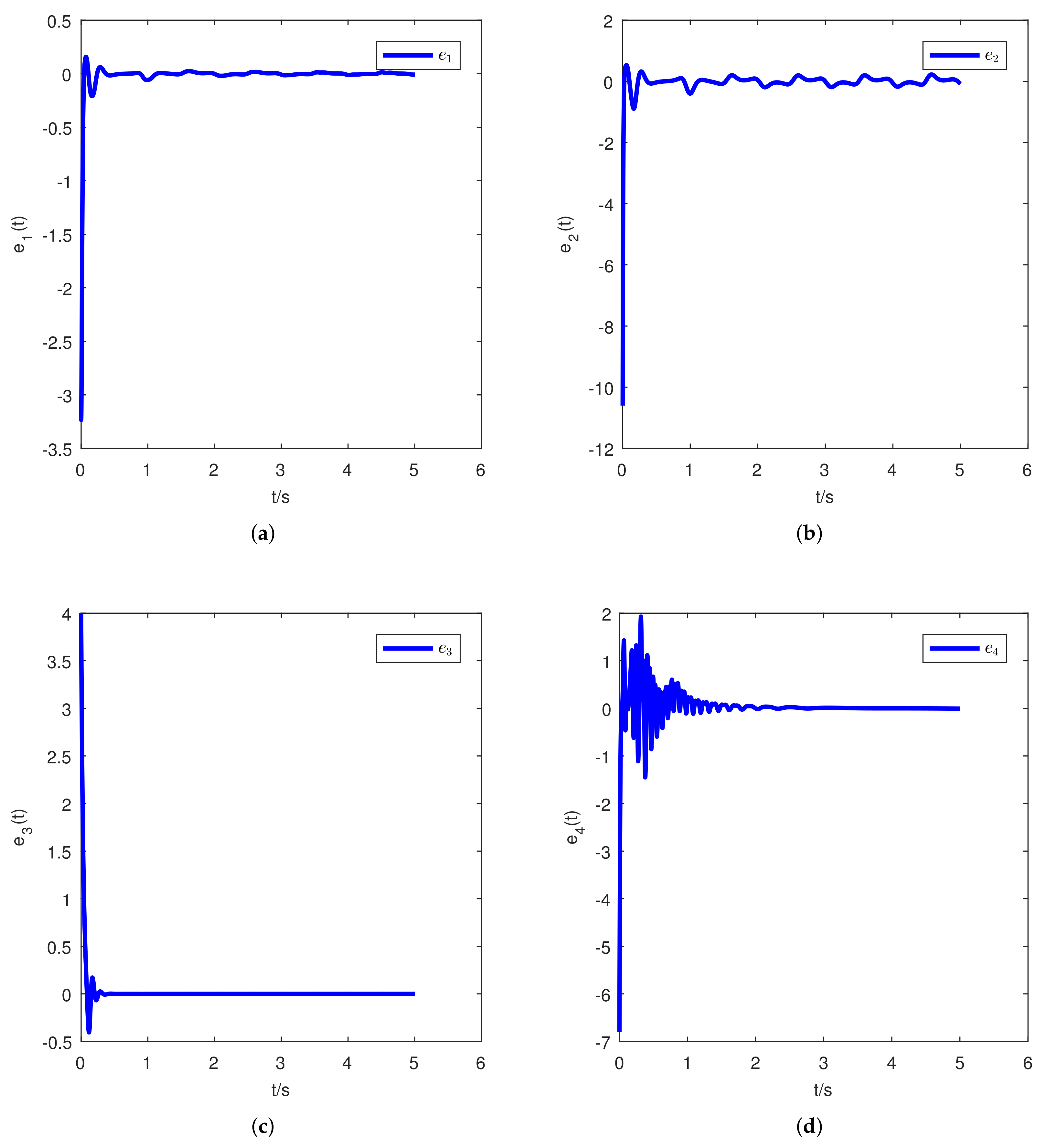
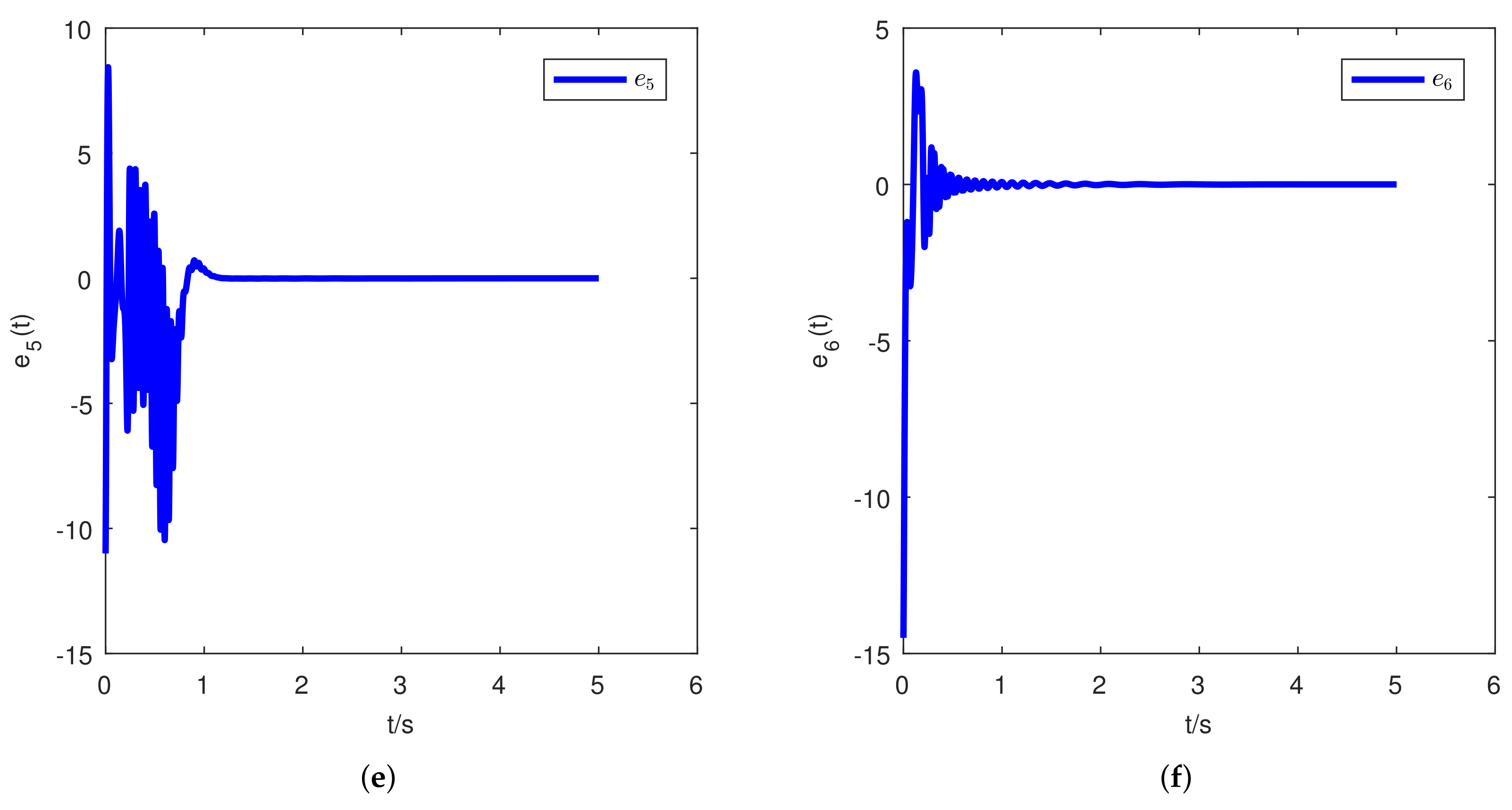
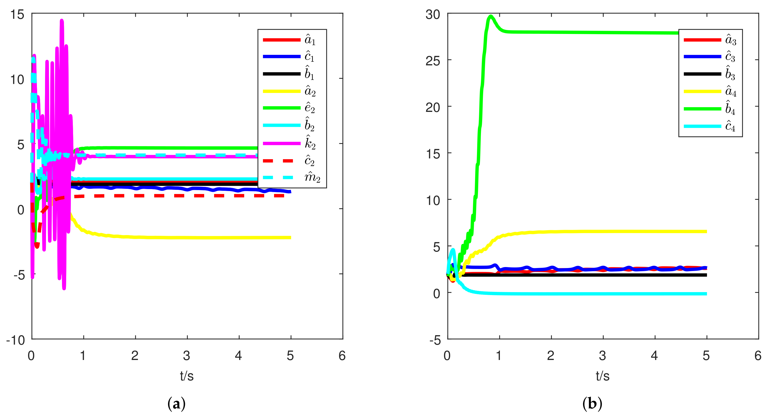
4.1. Adaptive Dual Synchronization of Chen, Lorenz, Liu and Lü Chaotic Systems

This part shows the adaptive dual synchronization of Chen, Lorenz, Liu and Lü fractional-order chaotic systems with unknown parameter, we use the Liu and Lü systems as the drive systems,
0 D t α x 11 ( t ) = a 1 ( x 12 x 11 ) , 0 D t α x 12 ( t ) = x 11 x 13 + c 1 x 12 , 0 D t α x 13 ( t ) = x 11 x 12 b 1 x 13 , 0 D t α x 14 ( t ) = a 2 x 14 e 2 x 15 2 , 0 D t α x 15 ( t ) = b 2 x 15 k 2 x 14 x 16 , 0 D t α x 16 ( t ) = c 2 x 16 + m 2 x 14 x 15 ,
where a 1 , c 1 , b 1 , a 2 , e 2 , b 2 , k 2 , c 2 , m 2 are system unknown parameters, and x 1 i ( t ) ( i = 1 , , 6 ) are the state vectors.
The driver systems in the form of Equation (25) is given as below:
D β x ( t ) = f ( x , t ) + F ( x ( t ) ) ρ ,
where f ( x , t ) = [ 0 , x 11 x 13 , x 11 x 12 , 0 , 0 , 0 ] T , ρ = [ a 1 , c 1 , b 1 , a 2 , e 2 , b 2 , k 2 , c 2 , m 2 ] T ,
F ( x ( t ) ) = ( x 12 x 11 ) 0 0 0 0 0 0 0 0 0 x 12 0 0 0 0 0 0 0 0 0 x 13 0 0 0 0 0 0 0 0 0 x 14 x 15 2 0 0 0 0 0 0 0 0 0 x 15 x 14 x 16 0 0 0 0 0 0 0 0 0 x 16 x 14 x 15 .
Chen and Lorenz systems with controllers are taken as response systems:
0 D t β y 11 ( t ) = a 3 ( y 12 y 11 ) + u 1 ( t ) , 0 D t β y 12 ( t ) = ( c 3 a 3 ) y 11 y 11 y 13 + c 3 y 12 + u 2 ( t ) , 0 D t β y 13 ( t ) = y 11 y 12 b 3 y 13 + u 3 ( t ) , 0 D t β y 14 ( t ) = a 4 ( y 15 y 14 ) + u 4 ( t ) , 0 D t β y 15 ( t ) = y 14 ( b 4 y 16 ) y 15 + u 5 ( t ) , 0 D t β y 16 ( t ) = y 14 y 15 c 4 y 16 + u 6 ( t ) ,
where a 3 , c 3 , b 3 , a 4 , b 4 , c 4 are system unknown parameters, and y 1 i ( t ) ( i = 1 , , 6 ) are the state vectors.
The response systems in the form of Equation (27) is given as follows:
D β y ( t ) = g ( y , t ) + G ( y ( t ) ) ν + U ( t ) ,
where
g ( y , t ) = 0 y 11 y 13 y 11 y 12 0 y 14 y 16 y 15 y 14 y 15 , ν = a 3 c 3 b 3 a 4 b 4 c 4 , U ( t ) = u 1 ( t ) u 2 ( t ) u 3 ( t ) u 4 ( t ) u 5 ( t ) u 6 ( t ) ,
G ( y ) = ( y 12 y 11 ) 0 0 0 0 0 y 11 y 11 + y 12 0 0 0 0 0 0 y 13 0 0 0 0 0 0 y 15 y 14 0 0 0 0 0 0 y 15 x 14 0 0 0 0 0 0 y 16 .
Suppose that e 1 = y 11 x 11 , e 2 = y 12 x 12 , e 3 = y 13 x 13 , e 4 = y 14 x 14 , e 5 = y 15 x 15 and e 6 = y 16 x 16 , so error dynamical system is described by:
D β e 1 ( t ) = a 3 ( y 12 y 11 ) a 1 ( x 12 x 11 ) , D β e 2 ( t ) = ( c 3 a 3 ) y 11 y 11 y 13 + c 3 y 12 + u 2 ( t ) ( x 11 x 13 + c 1 x 12 ) , D β e 3 ( t ) = y 11 y 12 b 3 y 13 + u 3 ( t ) ( x 11 x 12 b 1 x 13 ) , D β e 4 ( t ) = a 4 ( y 15 y 14 ) + u 4 ( t ) ( a 2 x 14 e 2 x 15 2 ) , D β e 5 ( t ) = y 14 ( b 4 y 16 ) y 15 + u 5 ( t ) ( b 2 x 15 k 2 x 14 x 16 ) , D β e 6 ( t ) = y 14 y 15 c 4 y 16 + u 6 ( t ) ( c 2 x 16 + m 2 x 14 x 15 ) .
Defining control function as:
u 1 ( t ) = a 3 ^ ( y 12 y 11 ) + a 1 ^ ( x 12 x 11 ) k 1 e 1 , u 2 ( t ) = x 11 x 13 + y 11 y 13 + a 3 ^ y 11 c 3 ^ ( y 11 + y 12 ) + c 1 ^ x 12 k 2 e 2 , u 3 ( t ) = x 11 x 12 y 11 y 12 + b 3 ^ y 13 b 1 ^ x 13 k 3 e 3 , u 4 ( t ) = a 4 ^ ( y 15 y 14 ) a 2 ^ x 14 e 2 ^ x 15 2 k 4 e 4 , u 5 ( t ) = y 14 y 16 + y 15 b 4 ^ y 14 + b 2 ^ x 15 k 2 ^ x 14 x 16 k 5 e 5 , u 6 ( t ) = y 14 y 15 + c 4 ^ y 16 + m 2 ^ x 14 x 15 k 6 e 6 ,
where a 1 ^ , b 1 ^ , c 1 ^ , e 2 ^ , b 2 ^ , a 2 ^ , k 2 ^ , c 2 ^ , m 2 ^ , b 3 ^ , c 3 ^ , a 3 ^ , b 4 ^ , a 4 ^ , c 4 ^ are estimated values for a 1 , b 1 , c 1 , e 2 , b 2 , a 2 , k 2 , c 2 , m 2 , b 3 , c 3 , a 3 , b 4 , a 4 , c 4 . The error dynamical system will be
D β e 1 ( t ) = ( a 3 a 3 ^ ) ( y 12 y 11 ) + ( a 1 ^ a 1 ) ( x 12 x 11 ) k 1 e 1 , D β e 2 ( t ) = ( c 1 ^ c 1 ) x 12 + ( a 3 ^ a 3 ) y 11 + ( c 3 c 3 ^ ) ( y 11 + y 12 ) k 2 e 2 , D β e 3 ( t ) = ( b 3 ^ b 3 ) y 13 + ( b 1 b 1 ^ ) x 13 k 2 e 2 , D β e 4 ( t ) = ( a 4 a 4 ^ ) ( y 15 y 14 ) + ( a 2 a 2 ^ ) x 14 + ( e 2 e 2 ^ ) x 15 2 k 4 e 4 , D β e 5 ( t ) = ( b 4 b 4 ^ ) y 14 + ( b 2 ^ b 2 ) x 15 + ( k 2 k 2 ^ ) x 14 x 15 k 5 e 5 , D β e 6 ( t ) = ( c 4 ^ c 4 ) y 16 + ( c 2 c 2 ^ ) x 16 + ( m 2 ^ m 2 ) x 14 x 15 k 6 e 6 ,
parameters update laws defined as:
D β a 1 ^ = e 1 ( x 12 x 11 ) , D β c 1 ^ = e 2 x 12 , D β b 1 ^ = e 3 x 13 , D β a 2 ^ = e 4 x 14 , D β e 2 ^ = e 4 x 15 2 , D β b 2 ^ = e 5 x 15 , D β k 2 ^ = e 5 x 14 x 16 , D β c 2 ^ = e 6 x 16 , D β m 2 ^ = e 6 x 15 x 14 , D β a 3 ^ = e 1 ( y 12 y 11 ) e 2 y 11 , D β c 3 ^ = e 2 ( y 11 + y 12 ) , D β b 3 ^ = e 3 y 13 , D β a 4 ^ = e 4 ( y 15 y 14 ) , D β b 4 ^ = e 5 y 14 , D β c 4 ^ = e 6 y 16 .
According to the above theory, the Lyapunov function is designed as:
V ( t ) = 1 2 ε ( t ) T ε ( t ) + 1 2 ρ ^ ρ 2 + 1 2 ν ^ ν 2 ,
and using Equations (30)–(32) results
D β v ( t ) k 1 e 1 2 k 2 e 2 2 k 3 e 3 2 k 4 e 4 2 k 5 e 5 2 k 6 e 6 2 < 0 .
Therefore, the stability condition of the error system based on Theorem 2 is obtained.
Assuming β = 0.995 , the values of parameters for which the systems (25) and (27) exhibits chaotic behaviour are taken as a 1 = 36 , c 1 = 20 , b 1 = 3 , a 2 = 1 , e 2 = 1 , b 2 = 2.5 , k 2 = 4 , c 2 = 5 , m 2 = 4 , a 3 = 35 , c 3 = 28 , b 3 = 3 , a 4 = 10 , b 4 = 28 , c 4 = 8 3 . The initial estimated values of parameters are taken as a 1 ^ = 2 , c 1 ^ = 2 , b 1 ^ = 2 , a 2 ^ = 2 , e 2 ^ = 2 , b 2 ^ = 2 , k 2 ^ = 2 , c 2 ^ = 2 , m 2 ^ = 2 , a 3 ^ = 2 , c 3 ^ = 2 , b 3 ^ = 2 , a 4 ^ = 2 , b 4 ^ = 2 , c 4 ^ = 2 , and the initial states of the drive and response systems when parameters are not known are arbitrarily chosen as x ( 0 ) = [ 0.2 , 7.6 , 1 , 7 , 11 , 15 ] T and y ( 0 ) = [ 3 , 3 , 5 , 0.2 , 0 , 0.5 ] T . We assume k i = 30 ( i = 1 , 2 , , 6 ) ; dual synchronization of the systems (25) and (27) and the variation of unknown parameters (32) are displayed in Figure 1 and Figure 2. Figure 1a–f reveals the dual synchronization errors, e i ( i = 1 , 2 , , 6 ) with time t. Figure 2a,b shows the change of predicted values of parameters a 1 ^ , c 1 ^ , b 1 ^ , a 2 ^ , e 2 ^ , b 2 ^ , k 2 ^ , c 2 ^ , m 2 ^ of drive systems (25) and a 3 ^ , c 3 ^ , b 3 ^ , a 4 ^ , b 4 ^ , c 4 ^ of response system (27).

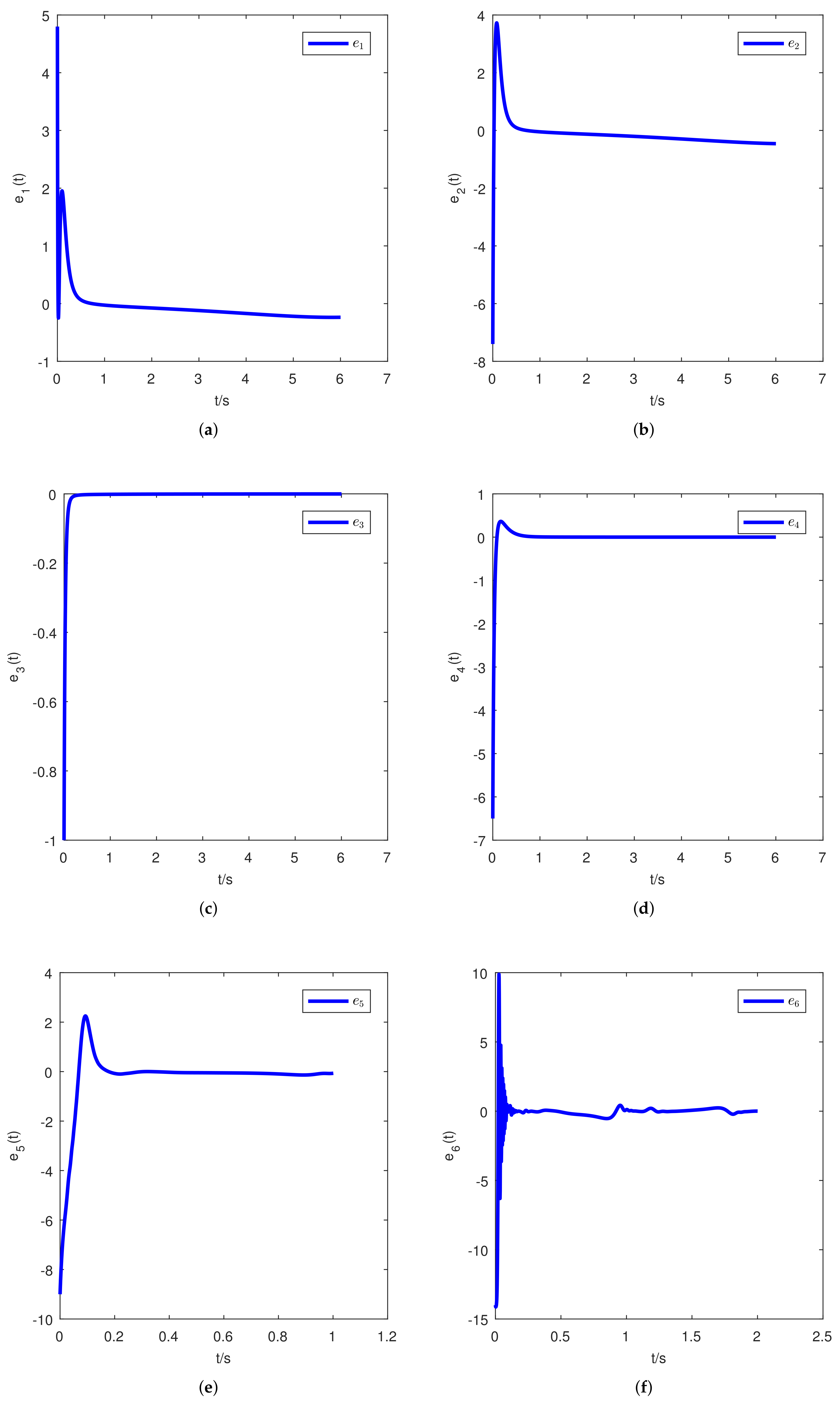
4.2. Adaptive Dual Synchronization of Chen, Lorenz, Lü and Liu Hyperchaotic Systems

In order to demonstrate the universality of the proposed method, we apply the proposed method to hyperchaotic systems. Similarly, we take the fractional Liu and Lü hyperchaotic systems as the driving systems,
0 D t β x 11 ( t ) = a 1 ( x 12 x 11 ) x 14 , 0 D t β x 12 ( t ) = x 11 x 13 c 1 x 12 , 0 D t β x 13 ( t ) = x 11 x 12 b 1 x 13 , 0 D t β x 14 ( t ) = x 11 x 13 r 1 x 14 , 0 D t β x 15 ( t ) = a 2 ( x 16 x 15 ) , 0 D t β x 16 ( t ) = b 2 x 15 k 2 x 15 x 17 + x 18 , 0 D t β x 17 ( t ) = h 2 x 15 2 c 2 x 17 + x 18 , 0 D t β x 18 ( t ) = e 2 x 16 ,
where a 1 , c 1 , b 1 , r 1 , a 2 , e 2 , b 2 , k 2 , c 2 , h 2 are system unknown parameters and x 1 i ( t ) , ( i = 1 , , 8 ) are the state vectors. When a 1 = 36 , b 1 = 3 , c 1 = 12 , r 1 = 0.4 of the fractional-order hyperchaotic Lü system parameters and 0.94 β 0.98 , the attractor of the system is hyperchaotic. When β = 0.96 , the Lyapunov exponents of Lü are λ 1 = 0.0023 , λ 2 = 0.202 , λ 3 = 0.0104 , λ 4 = 0.0115 [32]. When a 2 = 10 , b 2 = 40 , k 2 = 10 , h 2 = 4 , c 2 = 2.5 , e 2 = 2.5 of the fractional-order hyperchaotic Liu system parameters and 0 β 1 , the attractor of the system is hyperchaotic. When β = 1 , the Lyapunov exponents of Liu are λ 1 = 1.6639 , λ 2 = 0.0295 , λ 3 = 0.0274 and λ 4 = 14.1566 [33].
The driver systems in the form of Equation (35) is given as follows:
D β x ( t ) = f ( x , t ) + F ( x ( t ) ) ρ ,
where f ( x , t ) = [ x 14 , x 11 x 13 , x 11 x 12 , x 11 x 13 , 0 , x 18 , x 18 , 0 ] T , ρ = [ a 1 , c 1 , b 1 , r 1 , a 2 , b 2 , k 2 , h 2 , c 2 , e 2 ] T ,
F ( x ( t ) ) = ( x 12 x 11 ) 0 0 0 0 0 0 0 0 0 0 x 12 0 0 0 0 0 0 0 0 0 0 x 13 0 0 0 0 0 0 0 0 0 0 x 14 0 0 0 0 0 0 0 0 0 0 x 16 x 15 0 0 0 0 0 0 0 0 0 0 x 15 x 15 x 17 0 0 0 0 0 0 0 0 0 0 x 15 2 x 17 0 0 0 0 0 0 0 0 0 0 x 16 .
Chen and Lorenz hyperchaotic systems with controllers are taken as response systems:
0 D t α y 11 ( t ) = a 3 ( y 12 y 11 ) + y 14 + u 1 ( t ) , 0 D t α y 12 ( t ) = d 3 y 11 y 11 y 13 + c 3 y 12 + u 2 ( t ) , 0 D t α y 13 ( t ) = y 11 y 12 b 3 y 13 + u 3 ( t ) , 0 D t α y 14 ( t ) = y 12 y 13 + r 3 y 14 + u 4 ( t ) , 0 D t α y 15 ( t ) = a 4 ( y 16 y 15 ) + y 18 + u 5 ( t ) , 0 D t α y 16 ( t ) = c 4 y 15 y 15 y 17 y 16 + u 6 ( t ) , 0 D t α y 17 ( t ) = y 15 y 16 b 4 y 17 + u 7 ( t ) , 0 D t α y 18 ( t ) = y 16 y 17 + r 4 y 18 + u 8 ( t ) .
where a 3 , d 3 , c 3 , b 3 , r 3 , a 4 , c 4 , b 4 , r 4 are system unknown parameters, y 1 i ( t ) ( i = 1 , , 8 ) are the state vectors. When the parameters of Chen hyperchaotic system are a 3 = 35 , b 3 = 1 , c 3 = 12 , d 3 = 3 , r 3 = 0.4 , if 0.95 β 1 , the attractor of the system is hyperchaotic. When β = 0.97 , the Lyapunov exponents of Chen are λ 1 = 0.002 , λ 2 = 0.901 , λ 3 = 0.231 , λ 4 = 0.0008 [32]. When the parameters of Lorenz hyperchaotic system are a 4 = 10 , b 4 = 8 3 , c 4 = 28 , r 4 = 1 , if 0 β 1 , the attractor of the system is hyperchaotic. When β = 1 , the two positive Lyapunov exponents of Lorenz hyperchaotic system are λ 1 = 0.3985 , λ 2 = 0.2481 [34].
The response systems in the form of Equation (37) is given as follows:
D β y ( t ) = g ( y , t ) + G ( y ( t ) ) ν + U ( t ) .
where ν = [ a 3 , d 3 , c 3 , b 3 , r 3 , a 4 , c 4 , b 4 , r 4 ] T , g ( y , t ) = [ y 14 , y 11 y 13 , y 11 y 12 , y 12 y 13 , y 18 , y 15 y 17 y 16 , y 15 y 16 , y 16 y 17 ] T , U ( t ) = [ u 1 ( t ) , u 2 ( t ) , u 3 ( t ) , u 4 ( t ) , u 5 ( t ) , u 6 ( t ) , u 7 ( t ) , u 8 ( t ) ] T ,
G ( y ( t ) ) = ( y 12 y 11 ) 0 0 0 0 0 0 0 0 0 y 11 y 12 0 0 0 0 0 0 0 0 0 y 13 0 0 0 0 0 0 0 0 0 y 14 0 0 0 0 0 0 0 0 0 y 16 y 15 0 0 0 0 0 0 0 0 0 y 15 0 0 0 0 0 0 0 0 0 y 17 0 0 0 0 0 0 0 0 0 y 18 .
Suppose that e 1 = y 11 x 11 , e 2 = y 12 x 12 , e 3 = y 13 x 13 , e 4 = y 14 x 14 , e 5 = y 15 x 15 , e 6 = y 16 x 16 , e 7 = y 17 x 17 , and e 8 = y 18 x 18 , so error dynamical system is described by:
D β e 1 ( t ) = a 3 ( y 12 y 11 ) + y 14 a 1 ( x 12 x 11 ) + x 14 + u 1 ( t ) , D β e 2 ( t ) = d 3 y 11 y 11 y 13 + c 3 y 12 + x 11 x 13 + c 1 x 12 + u 2 ( t ) , D β e 3 ( t ) = y 11 y 12 b 3 y 13 x 11 x 12 + b 1 x 13 + u 3 ( t ) , D β e 4 ( t ) = y 12 y 13 + r 3 y 14 x 11 x 13 + r 1 x 14 + u 4 ( t ) , D β e 5 ( t ) = a 4 ( y 16 y 15 ) + y 18 a 2 ( x 16 x 15 ) + u 5 ( t ) , D β e 6 ( t ) = c 4 y 15 y 15 y 17 y 16 b 2 x 15 + k 2 x 15 x 17 x 18 + u 6 ( t ) , D β e 7 ( t ) = y 15 y 16 b 4 y 17 h 2 x 15 2 + c 2 x 17 x 18 + u 7 ( t ) , D β e 8 ( t ) = y 16 y 17 + r 4 y 18 + e 2 x 16 + u 8 ( t ) .
Control function is defined as:
u 1 ( t ) = x 14 y 14 a 3 ^ ( y 12 y 11 ) + a 1 ^ ( x 12 x 11 ) k 1 e 1 , u 2 ( t ) = x 11 x 13 + y 11 y 13 d 3 ^ y 11 c 3 ^ y 12 c 1 ^ x 12 k 2 e 2 , u 3 ( t ) = x 11 x 12 y 11 y 12 + b 3 ^ y 13 b 1 ^ x 13 k 3 e 3 , u 4 ( t ) = x 11 x 13 y 12 y 13 r 3 ^ y 14 r 1 ^ x 14 k 4 e 4 , u 5 ( t ) = y 18 a 4 ^ ( y 16 y 15 ) + a 2 ^ ( x 16 x 15 ) k 5 e 5 , u 6 ( t ) = x 18 + y 16 + y 15 y 17 c 4 ^ y 15 + b 2 ^ x 15 k 2 ^ x 15 x 17 k 6 e 6 , u 7 ( t ) = x 18 y 15 y 16 + b 4 ^ y 17 + h 2 ^ x 15 2 c 2 ^ x 17 k 7 e 7 , u 8 ( t ) = y 16 y 17 r 4 ^ y 18 e 2 ^ x 16 k 8 e 8 ,
where r 1 ^ , b 1 ^ , c 1 ^ , a 1 ^ , k 2 ^ , b 2 ^ , a 2 ^ , h 2 ^ , c 2 ^ , e 2 ^ , b 3 ^ , d 3 ^ , c 3 ^ , a 3 ^ , r 3 ^ , a 4 ^ , c 4 ^ , b 4 ^ , r 4 ^ are estimated values for r 1 , b 1 , c 1 , a 1 , k 2 , b 2 , a 2 , h 2 , c 2 , e 2 , b 3 , d 3 , c 3 , a 3 , r 3 , a 4 , c 4 , b 4 .
The error dynamical system will be:
D β e 1 ( t ) = ( a 3 a 3 ^ ) ( y 12 y 11 ) + ( a 1 ^ a 1 ) ( x 12 x 11 ) k 1 e 1 , D β e 2 ( t ) = ( c 1 c 1 ^ ) x 12 + ( d 3 d 3 ^ ) y 11 + ( c 3 c 3 ^ ) y 12 k 2 e 2 , D β e 3 ( t ) = ( b 3 ^ b 3 ) y 13 + ( b 1 b 1 ^ ) x 13 k 3 e 3 , D β e 4 ( t ) = ( r 3 r 3 ^ ) y 14 + ( r 1 r 1 ^ ) x 14 k 4 e 4 , D β e 5 ( t ) = ( a 4 a 4 ^ ) ( y 16 y 15 ) + ( a 2 ^ a 2 ) ( x 16 x 15 ) k 5 e 5 , D β e 6 ( t ) = ( c 4 c 4 ^ ) y 15 + ( b 2 ^ b 2 ) x 15 + ( k 2 k 2 ^ ) x 15 x 17 k 6 e 6 , D β e 7 ( t ) = ( b 4 ^ b 4 ) y 17 + ( h 2 ^ h 2 ) x 15 2 + ( c 2 c 2 ^ ) x 17 k 7 e 7 , D β e 8 ( t ) = ( r 4 r 4 ^ ) y 18 + ( e 2 e 2 ^ ) x 16 k 8 e 8 .
Parameters update laws are defined as:
D β a 1 ^ = e 1 ( x 12 x 11 ) , D β c 1 ^ = e 2 x 12 , D β b 1 ^ = e 3 x 13 , D β r 1 ^ = e 4 x 14 , D β a 2 ^ = e 5 ( x 16 x 15 ) , D β b 2 ^ = e 6 x 15 , D β k 2 ^ = e 6 x 15 x 17 , D β h 2 ^ = e 7 x 15 2 , D β c 2 ^ = e 7 x 17 , D β e 2 ^ = e 8 x 16 , D β a 3 ^ = e 1 ( y 12 y 11 ) , D β d 3 ^ = e 2 y 11 , D β c 3 ^ = e 2 y 12 , D β b 3 ^ = e 3 y 13 , D β r 3 ^ = e 4 y 14 , D β a 4 ^ = e 5 ( y 16 y 15 ) , D β c 4 ^ = e 6 y 15 , D β b 4 ^ = e 7 y 17 , D β r 4 ^ = e 8 y 18 .
The Lyapunov function is designed as:
V ( t ) = 1 2 ε ( t ) T ε ( t ) + 1 2 ρ ^ ρ 2 + 1 2 ν ^ ν 2 ,
and the results of Equations (40)–(42) are applied:
D β v ( t ) k 1 e 1 2 k 2 e 2 2 k 3 e 3 2 k 4 e 4 2 k 5 e 5 2 k 6 e 6 2 k 7 e 7 2 k 8 e 8 2 < 0 .
Therefore, the stability condition of the error system based on Theorem 2 is obtained.
For simulation, assuming β = 0.95 , the values of parameters for which the systems (35) and (37) exhibit chaotic behaviour are taken as a 1 = 36 , c 1 = 12 , b 1 = 3 , r 1 = 0.4 , a 2 = 10 , b 2 = 40 , k 2 = 2.5 , h 2 = 4 , c 2 = 2.5 , e 2 = 2.5 , a 3 = 35 , c 3 = 12 , b 3 = 3 , d 3 = 7 , r 3 = 0.5 , a 4 = 10 , b 4 = 8 3 , c 4 = 28 , r 4 = 1 . The initial estimated values of parameters are taken as a 1 ^ = 0 , c 1 ^ = 0 , b 1 ^ = 0 , r 1 ^ = 0 , a 2 ^ = 0 , b 2 ^ = 0 , k 2 ^ = 0 , h 2 ^ = 0 , c 2 ^ = 0 , e 2 ^ = 0 , a 3 ^ = 0 , d 3 ^ = 0 , c 3 ^ = 0 , b 3 ^ = 0 , r 3 ^ = 0 , a 4 ^ = 0 , c 4 ^ = 0 , b 4 ^ = 0 , r 4 ^ = 0 , and the initial states of the drive and response systems when parameters are not known are arbitrarily chosen as x ( 0 ) = [ 0.2 , 7.6 , 1 , 7 , 11 , 15 , 3 , 3 ] T and y ( 0 ) = [ 5 , 0.2 , 0 , 0.5 , 2 , 1 , 1 , 5 ] T . We consider k i = 30 ( i = 1 , 2 , , 8 ) ; dual synchronization of the systems (35) and (37) and the variation of unknown parameters (42) are displayed in Figure 3 and Figure 4. Figure 3a–h reveals the dual synchronization errors e i , ( i = 1 , 2 , , 8 ) with time t. Figure 3a,b shows the change of parameters’s predicted values a 1 ^ , c 1 ^ , b 1 ^ , r 1 ^ , a 2 ^ , b 2 ^ , k 2 ^ , h 2 ^ , c 2 ^ , e 2 ^ of drive systems (35) and a 3 ^ , d 3 ^ , c 3 ^ , b 3 ^ , r 3 ^ , a 4 ^ , c 4 ^ , b 4 ^ , r 4 ^ of response system (37).

5. Conclusions

Compared with the dual synchronization of most integer-order chaotic systems, an adaptive dual synchronization with unknown fractional order parameters is proposed in this paper. Based on Lyapunov stability theory, the adaptive controller (19) and adaptive law (20) are designed to realize the dual synchronization of two pairs of systems. Finally, two numerical simulation examples verify the effectiveness of the proposed method. Based on this research, we can consider the dual synchronization of fractional-order chaotic systems with interference in future research. In addition, we can also consider extending to chaotic system networks ( n > 2 ) and to less regular synchronization regimes, such as multi-clustering [35] and synchronization of a group of nodes [36], that is, the synchronization of multiple systems. Of course, there is still room for further thinking about follow-up research.

Author Contributions

D.L. proposed the main the idea and prepared the manuscript initially. T.L. gave the numerical simulation of this paper. Y.W. revised the English grammar of this paper. All authors have read and agreed to the published version of the manuscript.

Funding

This work is partly supported by the Project of the Science and Technology Department in Sichuan Province (Grant No.2019YJ0456, 2021ZYD0004), Fund of Sichuan University of Science and Engineering (Grant No. 2020RC26, 2020RC42).

Institutional Review Board Statement

Not applicable.

Informed Consent Statement

Not applicable.

Data Availability Statement

The data used to support the findings of this study are available from the corresponding author upon request.

Acknowledgments

The authors would like to thank the editor and the anonymous reviewers for their constructive comments and suggestions to improve the quality of the paper.

Conflicts of Interest

The authors declare that they have no competing interests.

References

  1. Butzer, P.L.; Westphal, U. An introduction to fractional calculus. Apidologie 2015, 33, 233–244. [Google Scholar]
  2. Miller, K.S.; Ross, B. An Introduction to the Fractional Calculus and Fractional Differential Equations; Wiley: Hoboken, NJ, USA, 1996; Volume 25, pp. 66–67. [Google Scholar]
  3. Li, C.L.; Yu, S.M.; Luo, X.S. Fractional-order permanent magnet synchronous motor and its adaptive chaotic control. Chin. Phys. B 2012, 21, 168–173. [Google Scholar] [CrossRef] [Green Version]
  4. Peterson, M.R.; Nayak, C. Effects of landau level mixing on the fractional quantum hall effect in monolayer graphene(Article). Phys. Rev. Lett. 2014, 113, 86401. [Google Scholar] [CrossRef] [PubMed] [Green Version]
  5. Rivero, M.; Rogosin, S.V.; Trujillo, J.J. Stability of Fractional Order Systems. Math. Probl. Eng. 2013, 2013, 133–174. [Google Scholar] [CrossRef]
  6. Dana, S.K.; Roy, P.K.; Kurths, J. Complex Dynamics in Physiological Systems: From Heart to Brain; Springer: Dordrecht, The Netherlands, 2009. [Google Scholar]
  7. Hilfer, R. Applications of Fractional Calculus in Physics; World Scientific: Singapore, Singapore, 2000. [Google Scholar]
  8. Podlubny, I. Fractional Differential Equations; Academic Press: Cambridge, MA, USA, 1999. [Google Scholar]
  9. Tao, Y.; Chua, L.O. Impulsive stabilization for control and synchronization of chaotic systems: Theory and application to secure communication. IEEE Trans. Circuits Syst. I Fundam. Theory Appl. 1997, 44, 976–988. [Google Scholar]
  10. Li, C.L.; Mei, Z.; Feng, Z. Projective synchronization for a fractional-order chaotic system via single sinusoidal coupling. Optik-Int. J. Light Electron Opt. 2016, 127, 2830–2836. [Google Scholar]
  11. Munozpacheco, J.M.; Posadascastillo, C.; Zambranoserrano, E. The Effect of a Non-Local Fractional Operator in an Asymmetrical Glucose-Insulin Regulatory System: Analysis, Synchronization and Electronic Implementation. Symmetry 2020, 1395, 1395. [Google Scholar] [CrossRef]
  12. Winkler, M.; Butsch, S.; Kinzel, W. Pulsed chaos synchronization in networks with adaptive couplings. Phys. Rev. Stat. Nonlinear & Soft Matter Phys. 2012, 86, 016203. [Google Scholar]
  13. Nicholasgeorge, J.; Selvamani, R. Modified projective synchronization between fractional order complex chaotic systems. J. Phys. Conf. Ser. 2020, 1597, 012015. [Google Scholar] [CrossRef]
  14. Li, C.C.; Kang, Z.J. Synchronization Control of Complex Network Based on Extended Observer and Sliding Mode Control. IEEE Access 2020, 8, 77336–77343. [Google Scholar]
  15. Nourian, A.; Balochian, S. The adaptive synchronization of fractional-order Liu chaotic system with unknown parameters. Pramana J. Phys. 2016, 86, 1401–1407. [Google Scholar] [CrossRef]
  16. Wang, Z.P.; Wu, H.N. Synchronization of chaotic systems using fuzzy impulsive control(Article). Nonlinear Dyn. 2014, 78, 729–742. [Google Scholar] [CrossRef]
  17. Yaghooti, B.; Shadbad, A.S.; Safavi, K.; Salarieh, H. Adaptive synchronization of uncertain fractional-order chaotic systems using sliding mode control techniques. Proc. Inst. Mech. Eng. Part I J. Syst. Control. Eng. 2020, 234, 3–9. [Google Scholar] [CrossRef]
  18. Tsimring, L.S.; Sushchik, M.M. Multiplexing chaotic signals using synchronization. Phys. Lett. A 1996, 213, 155–166. [Google Scholar] [CrossRef]
  19. Yun, L.; Davis, P. Dual synchronization of chaos. Phys. Rev. E 2000, 61, R2176–R2184. [Google Scholar]
  20. Han, L.X. Dual synchronization based on two different chaotic systems: Lorenz systems and Rössler systems. J. Comput. Appl. Math. 2006, 206, 1046–1050. [Google Scholar]
  21. Salarieh, H.; Shahrokhi, M. Dual synchronization of chaotic systems via time-varying gain proportional feedback. Chaos Solitons Fractals 2008, 38, 1342–1348. [Google Scholar] [CrossRef]
  22. Dibakar, G.; Roy, C.A. Dual-anticipating, dual and dual-lag synchronization in modulated time-delayed systems. Phys. Lett. A 2010, 374, 3425–3436. [Google Scholar]
  23. Sun, J.W.; Jiang, S.X.; Cui, G.Z.; Wang, Y. Dual Combination Synchronization of Six Chaotic Systems. J. Comput. Nonlinear Dyn. 2016, 11, 034501. [Google Scholar] [CrossRef]
  24. Mahmoud, G.M.; Farghaly, A.A.; Abed-Elhameed, T.M.; Darwish, M.M. Adaptive Dual Synchronization of Chaotic (Hyperchaotic) Complex Systems with Uncertain Parameters and Its Application in Image Encryption. Acta Phys. Pol. B 2018, 49, 1923–1939. [Google Scholar] [CrossRef]
  25. Ibraheem, A. Multi-switching Dual Combination Synchronization of Time Delay Dynamical Systems for Fully Unknown Parameters via Adaptive Control. Arab. J. Sci. Eng. 2020, 45, 6911–6922. [Google Scholar] [CrossRef]
  26. Li, Y.; Chen, Y.Q.; Podlubny, I. Mittag-Leffler stability of fractional order nonlinear dynamic systems. Automatica 2009, 45, 1965–1969. [Google Scholar] [CrossRef]
  27. Caponetto, R.; Ebrary, I. Fractional Order Systems: Modeling and Control Applications; World Scientific: Singapore, Singapore, 2010. [Google Scholar]
  28. Zhang, Q.; Xiao, J.; Zhang, X.Q.; Cao, D.Y. Dual projective synchronization between integer-order and fractional-order chaotic systems. Optik-Int. J. Light Electron Opt. 2017, 141, 90–98. [Google Scholar] [CrossRef]
  29. Vijay, K.Y.; Rakesh, K.; Subir, B.; Kumar, R. Dual phase and dual anti-phase synchronization of fractional order chaotic systems in real and complex variables with uncertainties. Chin. J. Phys. 2019, 57, 282–308. [Google Scholar]
  30. Aguila-Camacho, N.; Duarte-Mermoud, M.A.; Gallegos, J.A. Lyapunov functions for fractional order systems. Commun. Nonlinear Sci. Numer. Simul. 2014, 19, 2951–2957. [Google Scholar] [CrossRef]
  31. Li, Y.; Chen, Y.Q.; Podlubny, I. Stability of fractional-order nonlinear dynamic systems: Lyapunov direct method and generalized Mittag-Leffler stability. Comput. Math. Appl. 2009, 59, 1810–1821. [Google Scholar] [CrossRef] [Green Version]
  32. Sui, L.L. Hyperchaos and Synchronization of Fractional Chen and Lü Systems; Taiyuan University of Technology: Taiyuan, China, 2011. [Google Scholar]
  33. Liu, C.X. Fractional Order Chaotic Circuit Theory and Application; Xi’an Jiaotong University Press: Xi’an, China, 2011. [Google Scholar]
  34. Qiang, J. Projective synchronization of a new hyperchaotic Lorenz system. Phys. Lett. A 2007, 370, 40–45. [Google Scholar]
  35. Feketa, P.; Schaum, A.; Meurer, T. Synchronization and multi-cluster capabilities of oscillatory networks with adaptive coupling. IEEE Trans. Autom. Control 2020, 66, 1. [Google Scholar]
  36. Gambuzza, L.V.; Frasca, M.; Latora, V. Distributed Control of Synchronization of a Group of Network Nodes. IEEE Trans. Autom. Control 2018, 64, 365–372. [Google Scholar] [CrossRef]
Figure 1. (af): Error vector between drive system (25) and response system (27).
Mathematics 10 00470 g001aMathematics 10 00470 g001b
Figure 2. (a,b): Time response of estimated values of parameters a 1 ^ , c 1 ^ , b 1 ^ , a 2 ^ , e 2 ^ , b 2 ^ , k 2 ^ , c 2 ^ , m 2 ^ of drive systems (25) a 3 ^ , c 3 ^ , b 3 ^ , a 4 ^ , b 4 ^ , c 4 ^ of response system (27).
Mathematics 10 00470 g002
Figure 3. (ah): Error signals between drive system (35) and response system (37).
Mathematics 10 00470 g003aMathematics 10 00470 g003b
Figure 4. (a,b): Time response of estimated values of parameters a 1 ^ , c 1 ^ , b 1 ^ , r 1 ^ , a 2 ^ , b 2 ^ , k 2 ^ , h 2 ^ , c 2 ^ , e 2 ^ of drive systems (35) a 3 ^ , d 3 ^ , c 3 ^ , b 3 ^ , r 3 ^ , a 4 ^ , c 4 ^ , b 4 ^ , r 4 ^ of response system (37).
Mathematics 10 00470 g004
Publisher’s Note: MDPI stays neutral with regard to jurisdictional claims in published maps and institutional affiliations.

