Adaptive Sliding Mode Attitude-Tracking Control of Spacecraft with Prescribed Time Performance

Abstract

In this article, a novel finite-time attitude-tracking control scheme is proposed by using the prescribed performance control (PPC) method for the spacecraft system under the external disturbance and an uncertain inertia matrix. First, a novel polynomial finite-time performance function (FTPF) was used to avoid the complex calculation of exponential function from conventional FTPF. Then, a simpler error transformation was introduced to guarantee that the attitude-tracking error converges to a preselected region in prescribed time. Subsequently, a robust adaptive controller was proposed by using the backstepping method and the sliding mode control (SMC) technique. Unlike the existing attitude-tracking control results, the proposed PPC scheme guarantees the performance of spacecraft system under the static and transient conditions. Meanwhile, the state trajectory of system can be completely drawn into the designed sliding surface. The stability of the control scheme is proven rigorously by the Lyapunov’s theory of stability. Finally, the simulations show that the convergence rate and the convergence accuracy are better for the tracking errors of spacecraft system under the proposed control scheme.

1. Introduction

Over the past several decades, the attitude-tracking control of spacecraft systems has been extensively investigated due to its extensive applications during the execution of space missions, such as earth imaging, spacecraft docking and rendezvous, satellite surveillance and multiorbit task, etc. Thus, many effective developments have emerged [1,2,3,4,5,6,7,8]. It is worth noting that, in the practical space tasks, the kinematics and dynamics of spacecraft system have strong coupling and high nonlinearity, which results in uncertainties of system model. At the same time, the external disturbance inevitably occurs in the spacecraft system which leads to poor efficiency or instability. For these reasons, achieving the accurate attitude-tracking control of the spacecraft system has became a challenging problem. A large number of effective nonlinear control methods, for instance, the adaptive control [9,10,11,12], the fuzzy control [13,14,15], and the sliding mode control (SMC) [16,17,18,19,20], etc., have been proposed to address the above problems.

Among the aforementioned control methods, the SMC technique has been extensively used in the attitude-tracking control of the spacecraft system to resolve the issues of high nonlinearity and strong coupling. For example, a variable structure SMC technology was proposed firstly to achieve the stabilization of angular velocity for the multiaxial spacecraft in [21]. Then, a modified higher-order SMC law was proposed to realize the high-pointing accurate control in [22]. By combining the SMC technology and the adaptive control method, [23,24,25] addressed the attitude-tracking control issue of spacecrafts with an unknown inertia matrix and the external disturbance. Furthermore, by the Rodrigues parameter representation, [26] designed a neuroadaptive SMC controller to achieve the stabilization of the spacecraft system. Reference [27] studied a fuzzy SMC scheme to realize the attitude-tracking control of the spacecraft with the unknown nonlinear term. However, the above-mentioned control strategies only guaranteed that the attitude-tracking error converges to a vicinity of the origin in the infinite-time interval. In order to fulfill the convergence within finite time, the authors designed a terminal sliding mode (TSM) in [28] where the proposed control method forces the sliding surface into a compact set of the origin point within an interval of time. With the help of the TSM and the neural network technology, the finite-time stability of the attitude-tracking error could be guaranteed [29]. Nevertheless, the proposed control schemes only guaranteed that the state trajectory of system is drawn into the neighborhood of the sliding surface. In addition, these results could only achieve the steady-state performance of spacecraft system, while the transient-state performance is also a major concern during the operation of the spacecraft.

In the case of ensuring the stability of the conversion error system, the prescribed performance control (PPC) was proposed [30] to achieve the tracking performance under the static and transient conditions. After that, some representative results were made [31,32,33,34,35,36,37]. A robust adaptive controller with the prescribed performance function (PPF) in [30] was presented for the nonlinear system, such that the tracking error converged to a preselected adjustable area by choosing appropriate parameters. In order to make the tracking error converge to a range within the prescribed time, the finite-time performance function (FTPF) was proposed [34] where the tracking error could converge to an area in prescribed time for a class of an uncertain system. By the aid of the FTPF and the neural networks in [35], the finite-time tracking control was properly realized for the nonlinear system in the form of nonstrict feedback. Combined with the FTPF, an adaptive PPC scheme [36] was presented to settle the finite-time attitude-tracking issue of the spacecraft system. For the spacecraft system with an unknown disturbance, a prescribed-time adaptive controller [37] was designed by using the FTPF and the SMC technology. It is worth emphasizing that the above FTPF [34,35,36,37] was an exponential form, which would produce an additional coupling term in the transformed dynamic equation.

To the author’s knowledge, there is little research about the prescribed-time attitude-tracking control for the spacecraft system. What is more, few results show that the state trajectory of system is completely drawn into the designed sliding surface. Inspired by the above discussions, the prescribed-time attitude-tracking problem continues to study by using the PPC method and the SMC technology, and the external disturbance and an uncertain inertia matrix are considered simultaneously in this article. A prescribed-time adaptive SMC strategy is proposed to achieve the accurate attitude-tracking of the spacecraft by using the backstepping method. The main innovations are summarized as below:

(i)

Different from the previous SMC works [21,22,23,24,25,26,27,28,29], a novel robust adaptive controller with prescribed performance is designed to guarantee that the state trajectory of system is drawn into the designed sliding surface completely by the approach of bounded estimation;

(ii)

Unlike the PPC results [34,35,36,37], a novel FTPF is introduced to avoid the complicated calculation of exponential function from the conventional FTPF. Meanwhile, the attitude-tracking error can converge to a preselected adjustable boundary in prescribed time;

(iii)

The first-order sliding mode differentiator (FOSD) is used to solve the issue of “explosion of complexity" caused by the traditional backstepping method. The proposed control scheme avoids the calculation of the derivative for the virtual controller and greatly reduces the computational burden.

The rest of the article is structured in the following ways: The description of spacecraft system and some preparatory works are presented in Section 2. A novel polynomial FTPF is used in Section 3, then a transformed error system is presented by utilizing the error transformation technique, and a robust adaptive controller is proposed by using the backstepping method and the SMC technology. The numerical simulations are showed in Section 4. The conclusion is drawn in Section 5. Some remarks are presented in each section.

2. Model Description and Problem Statement

2.1. Notation

Throughout this article, the following notations are used. For a given vector $a=[a_1$ $a_2$ $\dots$$a_n{]}^T\in {\mathbb{R}}^n$, its norm is defined as $\parallel a\parallel =\sqrt{a^{T}a}$. For any $a\in {\mathbb{R}}^n$, $b\ge 0$, $\left|a\right|=\left[\right|a_1|,$ $|a_2|,$ $\dots ,|a_n{\left|\right]}^T$, $sgn\left(a\right)=[sgn\left(a_1\right),$ $sgn\left(a_2\right),\dots ,$ $sgn\left(a_n\right){]}^T$, and $sig{n}^b\left(a\right)=\left[\right|a_1{|}^{b}sign\left(a_1\right),$ $|a_2{|}^{b}sign\left(a_2\right),$ $\dots ,|a_3{{|}^{b}sign\left(a_n\right)]}^T$. $sign(·)$ is the signum function. $exp(·)$ denotes the exponential function, and the base of the exponential function is the natural constant e. For a given matrix $A\in {\mathbb{R}}^{n\times n}$, its norm is defined as $\parallel A\parallel =\sqrt{{\left(A^{T}A\right)}_M}$, in which $A_M$ denotes the largest eigenvalue of matrix A. $I_N\in {\mathbb{R}}^{N\times N}$ denotes an identity matrix; ${}^{\times }$ is a calculation to the vector $c={\left[c_1{c}_2{c}_3\right]}^T\in {\mathbb{R}}^3$ such that:

$$c^{\times }=\left[\begin{array}{ccc}0& -c_3& c_2\\ c_3& 0& -c_1& \\ -c_2& c_1& 0\end{array}\right].$$

(1)

2.2. Attitude Dynamics and Kinematics of Speerschaft

The dynamic and kinematic equations of the spacecraft system are described as:

$$\begin{array}{c}\hfill \dot{q}=\frac{1}{2}(q_4{I}_3+q^{\times })\Omega {\dot{q}}_4=-\frac{1}{2}{q}^{\mathrm{T}}\Omega J\dot{\Omega }=-{\Omega }^{\times }J\Omega +u+d\end{array}$$

(2)

where the attitude orientation of spacecraft system is defined as the unit quaternion $q_v=[q_1$ $q_2$ $q_3$ $q_4{]}^T={\left[q^T{q}_4\right]}^T$, $q=[q_1$ $q_2$ $q_3{]}^T\in {\mathbb{R}}^3$ is a form of vector, $q_4\in \mathbb{R}$ is a a form of scalar, and q satisfies $q^{T}q+{q_4}^2=1$. $\Omega =[{\Omega }_1$${\Omega }_2$${\Omega }_3{]}^T\in {\mathbb{R}}^3$ is the angular velocity of the spacecraft system. $J\in {\mathbb{R}}^{3\times 3}$ denotes an inertial matrix which is symmetric and positive definite. $u=[u_1$$u_2$$u_3{]}^T$$\in {\mathbb{R}}^3$ denotes the input vector, and $d=[d_1$$d_2$$d_3{]}^T$$\in {\mathbb{R}}^3$ denotes the external disturbance.

2.3. Relative Attitude Error Dynamics and Kinematics

The desired attitude orientation of the spacecraft system is defined as $q_{dv}={[q_d^T,q_{d4}]}^T$, and $q_d={[q_{d1},q_{d2},q_{d3}]}^T$ represents the desired attitude. The unit quaternion $q_{dv}$ satisfies $\parallel q_{dv}\parallel =1$. Accordingly, $q_{ev}={[q_e^T,q_{e4}]}^T$ is the relative error from the body-fixed reference frame to the desired reference frame, $q_e={[q_{e1},q_{e2},q_{e3}]}^T$ is the attitude-tracking error. The unit quaternion $q_{ev}$ satisfies $\parallel q_{ev}\parallel =1$, $q_e=q_{d4}q-q_d^{\times }q-q_4{q}_d$, $q_{e4}=q_d^{T}q+q_4{q}_{d4}$. The desired angular velocity is defined as ${\Omega }_d$. ${\Omega }_e=\Omega -C{\Omega }_d$ denotes the bounded angular velocity tracking error, and $C=(q_{e4}^2-q_e^T{q}_e)I_3+2q_e{q}_e^T-2q_{e4}{q}_e^{\times }$$(\parallel C\parallel =1,\dot{C}=-{\Omega }_e^{\times }C)$ is the corresponding matrix of rotation. Assuming that the full states can be obtained and ${\Omega }_d$ and ${\dot{\Omega }}_d$ are all bounded, the relative attitude error dynamic and kinematic equations are described as:

$$\begin{array}{cc}\hfill & {\dot{q}}_e=\frac{1}{2}(q_{e4}{I}_3+q_e^{\times }){\Omega }_e{\dot{q}}_{e4}=-\frac{1}{2}{q}_v^T{\Omega }_e\hfill \\ \hfill & J{\dot{\Omega }}_e=-{({\Omega }_e+C{\Omega }_d)}^{\times }J({\Omega }_e+C{\Omega }_d)+J({\Omega }_e^{\times }C{\Omega }_d-C\dot{{\Omega }_d})+u+d\hfill \end{array}$$

(3)

Remark 1.

The kinematics and dynamics of spacecraft system can be generally expressed by the Rodrigues representation or the quaternion representation. The Rodrigues representation provides three dimensional parameterizations. However, a singularity exists during the process of spacecraft. To avoid this problem, the quaternion representation is introduced in this article.

2.4. Problem Statement

In this paper, the control target is to study a robust adaptive prescribed performance control (PPC) scheme such that: (1) the boundedness of all signals is ensured; and (2) the attitude-tracking error $q_e$ can converge to a preselected adjustable boundary in prescribed time, which can be expressed by the following inequality:

$$-{\mu }_l\beta \left(t\right)\le q_{ei}\left(t\right)\le {\mu }_h\beta \left(t\right),i=1,2,3,t\ge T_r$$

(4)

where ${\mu }_l>0$, ${\mu }_h>0$ are positive constants, $\beta \left(t\right)$ is the prescribed performance function, $-{\mu }_l\beta \left(t\right)$ and ${\mu }_h\beta \left(t\right)$ are the preselected boundaries of the attitude-tracking error, and $T_r$ is the prescribed time. To achieve the control target, the assumptions and lemmas are served as references in the following content.

Assumption 1.

The norm of the inertial matrix is assumed to have an upper bound:

$$\begin{array}{c}\hfill \parallel J\parallel \le \theta \end{array}$$

(5)

where θ is a known positive constant.

Remark 2.

Due to the fuel consumption, motor overload, and other factors, many characteristics of the spacecraft system are uncertain. These factors may cause the inertial matrix to be uncertain. Even if the inertial matrix is uncertain, it is still bounded.

Assumption 2.

The external disturbance $d\left(t\right)$ is assumed to be bounded such that:

$$\begin{array}{c}\hfill \parallel d\left(t\right)\parallel \le l_d\end{array}$$

(6)

where $l_d$ is a known positive constant.

Lemma 1.

([38]). The first-order sliding mode differentiator (FOSD) is defined as follows:

$$\begin{array}{c}\hfill {\dot{\varpi }}_0={\iota }_0=-{ϵ}_0{|{\varpi }_0-\varrho \left(t\right)|}^{1/2}sign({\varpi }_0-\varrho \left(t\right))+{\varpi }_1{\dot{\varpi }}_1=-{ϵ}_{1}sign({\varpi }_1-{\dot{\varpi }}_0)\end{array}$$

(7)

where the states of system are ${\varpi }_0$ and ${\varpi }_1$, the derivative of ${\varpi }_0$ is ${\iota }_0$, ${ϵ}_0$ and ${ϵ}_1$ are positive parameters, $\varrho \left(t\right)$ is the input, and the differential term $\varrho \left(t\right)$ can be replaced by ${\iota }_0$ when the initial errors ${\varpi }_0-\varrho \left(t_0\right)$ and ${\iota }_0-\dot{\varrho }\left(t_0\right)$ are bounded.

Lemma 2.

([39]). If $g:{\mathbb{R}}^{+}\to \mathbb{R}$ is a continuous function uniformly when $t\ge 0$ and the integral $\underset{t\to \infty }{lim}{\int }_0^t\left|g\left(\tau \right)d\tau \right|$ is finite and exists, then:

$$\begin{array}{c}\hfill \underset{t\to \infty }{lim}g\left(t\right)=0\end{array}$$

(8)

3. Controller Design and Stability Analysis

In this section, a robust adaptive PPC control scheme is proposed to solve the finite-time attitude-tracking control problem for the normal error system (3) by using the backstepping method and the sliding mode control (SMC) technique. Before the procedure of backstepping method, a novel FPTF is introduced, and the error transformation is used for the purpose of guaranteeing prescribed tracking performance.

3.1. Novel Finite-Time Performance Function (FTPF)

In the existing PPC methods [34,35,36,37], the formulation of prescribed performance is expressed as:

$$-k_l\beta \left(t\right)\le q_{ei}\left(t\right)\le k_h\beta \left(t\right)$$

(9)

where $k_l>0$ and $k_h>0$ are positive constants and $\beta \left(t\right)$ is the FTPF, which is always chosen as:

$${\beta }_{old}\left(t\right)=\left\{\begin{array}{cccc}\hfill ({\beta }_0-{\beta }_{\infty })exp(-l\frac{T_{r}t}{T_r-t})+{\beta }_{\infty },& \hfill & & t\in [0,T_r)\hfill \\ \hfill {\beta }_{\infty },& \hfill & & t\in [T_r,\infty )\hfill \end{array}\right.$$

(10)

where ${\beta }_0>{\beta }_{\infty }>0$ are positive constants, $0<T_r<\infty$ is the prescribed time, and $l>0$ is an adjustable parameter that can affect the performance of the conventional FTPF.

In this subsection, a novel polynomial FTPF is proposed as:

$$\beta \left(t\right)=\left\{\begin{array}{cccc}\hfill k_3{t}^3+k_2{t}^2+k_{1}t+k_0,& \hfill & & t\in [0,T_r]\hfill \\ \hfill {\beta }_{Tr},& \hfill & & t\in (T_r,\infty )\hfill \end{array}\right.$$

(11)

Meanwhile, $k_0,k_1,k_2$ and $k_3$ satisfy the following equations:

$$\left\{\begin{array}{c}\beta \left(0\right)=k_0={\beta }_n\hfill \\ \beta \left(T_r\right)=k_3{T}_r^3+k_2{T}_r^2+k_1{T}_r+k_0={\beta }_{Tr}\hfill \\ \dot{\beta }\left(T_r\right)=3k_3{T}_r^2+2k_2{T}_r+k_1=0\hfill \\ \ddot{\beta }\left(T_r\right)=6k_3{T}_r+2k_2=0\hfill \end{array}\right.$$

(12)

Then, $k_0,k_1,k_2$ and $k_3$ can be solved as:

$$\left\{\begin{array}{c}{k}_0={\beta }_n\hfill \\ k_1=-\frac{3}{T_r}({\beta }_n-{\beta }_{Tr})\hfill \\ k_2=\frac{3}{T_r^2}({\beta }_n-{\beta }_{Tr})\hfill \\ k_3=-\frac{1}{T_r^3}({\beta }_n-{\beta }_{Tr})\hfill \end{array}\right.$$

(13)

where ${\beta }_n>{\beta }_{Tr}>0$ are positive and $T_r$ is the prescribed time.

The parameters of ${\beta }_{old}\left(t\right)$ are selected as $T_r=10$, ${\beta }_0=1$, and ${\beta }_{\infty }=0.05$, and l is set as $0.2,$ $0.1,$ and $0.05$, respectively. The parameters of $\beta \left(t\right)$ are selected as $T_r=10$, ${\beta }_n=1$, and ${\beta }_{Tr}=0.05$. The comparison of novel FTPF and conventional FTPF is shown in Figure 1.

Remark 3.

Unlike the conventional FTPF in [34,35,36,37], the novel FTPF has three main advantages: (1) The prescribed performance function $\beta \left(t\right)$ monotonously decreases when $0<t<T_r$, $\beta \left(t\right)$ can converge to ${\beta }_{Tr}$ in prescribed time $T_r$, and $\beta \left(t\right)={\beta }_{Tr}$ when $t>T_r$. (2) The novel function is a simple polynomial form, and its derivative is continuous and smooth. (3) The novel FTPF does not involve the singularity and the chattering phenomenon which are produced by the exponential term.

It is clear that the novel FTPF is smoother and faster than the conventional FTPF. The novel FTPF can achieve the prescribed-time convergence, and it can converge to a preselected adjustable boundary and stay within this boundary.

3.2. Error Transformation

Due to constraint (4), it is difficult to design a controller to achieve the control target. Therefore, the following error transformation is defined to transform the constrained control problem into the unconstrained control problem.

Next, a new vector ${\overline{q}}_e\left(t\right)=$$[{\overline{q}}_{e1}$ ${\overline{q}}_{e2}$${\overline{q}}_{e3}]$$\in {\mathbb{R}}^3$ is introduced as follows:

$$\begin{array}{c}\hfill {\overline{q}}_{ei}\left(t\right)=\frac{2}{{\mu }_l+{\mu }_h}(\frac{q_{ei}\left(t\right)}{\beta \left(t\right)}-\frac{{\mu }_h-{\mu }_l}{2}),i=1,2,3\end{array}$$

(14)

where $\beta \left(t\right)$ is the novel FTPF in (11).

According to Formulas (4) and (14), ${\overline{q}}_{ei}\left(t\right)$ satisfies the following inequality:

$$\begin{array}{c}\hfill -1<{\overline{q}}_{ei}\left(t\right)<1\end{array}$$

(15)

Hence, the transformed error function $\varsigma \left({\varphi }_{ei}\left(t\right)\right)$ should have the following characteristics:

$$\left\{\begin{array}{c}1<\varsigma \left({\varphi }_{ei}\left(t\right)\right)<1\hfill \\ \underset{{\varphi }_{ei}\left(t\right)\to +\infty }{lim}\varsigma \left({\varphi }_{ei}\left(t\right)\right)=1\hfill \\ \underset{{\varphi }_{ei}\left(t\right)\to -\infty }{lim}\varsigma \left({\varphi }_{ei}\left(t\right)\right)=-1\hfill \end{array}\right.$$

(16)

where ${\varphi }_e={[{\varphi }_{e1},{\varphi }_{e2},{\varphi }_{e3}]}^T$ is the transformed error.

To satisfy (16), the transformed error function $\varsigma \left({\varphi }_{ei}\left(t\right)\right)$ is constructed as:

$$\begin{array}{c}\hfill {\overline{q}}_{ei}\left(t\right)=\varsigma \left({\varphi }_{ei}\left(t\right)\right)=\frac{2}{\pi }arctan\left({\varphi }_{ei}\left(t\right)\right)\end{array}$$

(17)

In [34], $\varsigma \left({\varphi }_{ei}\left(t\right)\right)$ is a strictly monotonic function. According to the existing condition of the inverse function, $\varsigma \left({\varphi }_{ei}\left(t\right)\right)$ has an inverse function ${\varphi }_e\left(t\right)$. Thus, the transformed attitude-tracking error ${\varphi }_e\left(t\right)$ can be presented as:

$$\begin{array}{c}\hfill {\varphi }_e\left(t\right)=tan\left(\frac{\pi }{2}{\overline{q}}_e\left(t\right)\right)\end{array}$$

(18)

Hence, $q_e\left(t\right)$ can be replaced by the new vector ${\varphi }_e\left(t\right)$ during the design of the controller. From Formulas (3), (14) and (18), it can be gathered that:

$$\begin{array}{c}\hfill {\dot{\varphi }}_e\left(t\right)=P_s({\dot{q}}_e\left(t\right)+\gamma )\end{array}$$

(19)

where $\gamma =[{\gamma }_1$${\gamma }_2$${\gamma }_3{]}^T$$\in {\mathbb{R}}^3$ and

$$\left\{\begin{array}{c}{P}_s=diag[p_{s1},p_{s2},p_{s3}]\hfill \\ p_{si}=\frac{\pi }{({\mu }_l+{\mu }_h)\beta \left(t\right)}[1+ta{n}^2\left(\frac{\pi }{2}{\overline{q}}_{ei}\right)],i=1,2,3\hfill \\ {\gamma }_i=-\frac{q_{ei}\dot{\beta }\left(t\right)}{\beta \left(t\right)},i=1,2,3\hfill \end{array}\right.$$

(20)

Remark 4.

In this article, the choice of ${\beta }_n,{\beta }_{Tr}$ and $T_r$ is important for the attitude-tracking performance. ${\beta }_n$ can limit the initial value of attitude-tracking error; ${\beta }_{Tr}$ can control the tracking accuracy of attitude-tracking error; and $T_r$ can control the convergence time of the attitude-tracking error. Moreover, the prescribed time is independent of other parameters; thus, it can be assigned to any values.

3.3. Controller Design

In this subsection, a robust adaptive PPC control scheme is presented to solve the attitude-tracking control problem for the normal error system (3) by using the backstepping method. The following auxiliary variables are introduced:

$$\begin{array}{c}\hfill z_1={\varphi }_e{z}_2={\Omega }_e-\alpha \left({\varphi }_e\right)\end{array}$$

(21)

where $\alpha \left({\varphi }_e\right)$ is defined as the virtual controller.

Step 1: By Formulas (3) and (19), the derivative of $z_1$ can be obtained such that:

$$\begin{array}{c}\hfill {\dot{z}}_1=P_s({\dot{q}}_e\left(t\right)+\gamma )=P_s(T{\Omega }_e+\gamma )=P_s(T(z_2+\alpha \left({\varphi }_e\right))+\gamma )\end{array}$$

(22)

where $T=\frac{1}{2}(q_4{I}_3+q^{\times })$.

To stabilize Formula (22), the candidate Lyapunov function is chosen as:

$$\begin{array}{c}\hfill V_1=\frac{1}{2}{z}_1{\left(t\right)}^T{z}_1\left(t\right)\end{array}$$

(23)

where $z_1={\varphi }_e\left(t\right)$ is the transformed attitude-tracking error. It can be noticed that $q_e\left(t\right)$ satisfies constraint (4) when ${\varphi }_e\left(t\right)$ is bounded.

In the following, the virtual control law $\alpha \left({\varphi }_e\right)$ is designed as:

$$\begin{array}{c}\hfill \alpha \left({\varphi }_e\right)=-T^{-1}[K_a{\left({\varphi }_e^T{P}_s\right)}^T+\gamma ]\end{array}$$

(24)

where $K_a$ is a positive definite and symmetric matrix.

Along Formulas (23) and (24), the derivative of $V_1$ can be given as:

$$\begin{array}{c}\hfill \dot{V_1}={\varphi }_e^T{P}_{s}T{z}_2-\left({\varphi }_e^T{P}_s\right)K_a{\left({\varphi }_e^T{P}_s\right)}^T=-\left(z_1^T{P}_s\right)K_a{\left(z_1^T{P}_s\right)}^T+z_1^T{P}_{s}T{z}_2\end{array}$$

(25)

Step 2: In this step, the SMC technology and the approach of bounded estimation are proposed to guarantee that the state trajectory of system can be completely drawn from the outside into the inside of the sliding surface. The sliding surface is chosen as:

$$\begin{array}{cc}\hfill & S=z_2={\Omega }_e-\alpha =0\hfill \end{array}$$

(26)

where $S=[S_1$$S_2$$S_3]\in {\mathbb{R}}^3$ is a vector.

According to error system (3), the derivative of (26) can be obtained as:

$$\begin{array}{c}\hfill J\dot{S}=J{\dot{\Omega }}_e-J\dot{\alpha }=-{({\Omega }_e+C{\Omega }_d)}^{\times }J({\Omega }_e+C{\Omega }_d)+J({\Omega }_e^{\times }C{\Omega }_d-C\dot{{\Omega }_d})+u+d-J\dot{\alpha }\end{array}$$

(27)

To avoid the complicated calculation, the FOSD is presented to estimate the $\dot{\alpha }$:

$$\begin{array}{c}\hfill {\dot{\varpi }}_0={\iota }_0=-{ϵ}_0{|{\varpi }_0-\alpha |}^{1/2}sign({\varpi }_0-\alpha )+{\varpi }_1{\dot{\varpi }}_1=-{ϵ}_{1}sign({\varpi }_1-{\dot{\varpi }}_0)\end{array}$$

(28)

where ${\varpi }_0,{\varpi }_1$ are state, and ${ϵ}_0$ and ${ϵ}_1$ are positive parameter.

From Lemma 2, we can obtain that:

$$\begin{array}{cc}\hfill & \dot{\alpha }={\dot{\varpi }}_0+\Delta \dot{\alpha }\hfill \end{array}$$

(29)

where $\Delta \dot{\alpha }$ denotes the estimated error of FOSD with $\parallel \Delta \dot{\alpha }\parallel \le {\alpha }_1$ and ${\alpha }_1>0$ denotes the upper boundary of the estimated error.

Remark 5.

$\parallel \Delta \dot{\alpha }\parallel \le {\alpha }_1$ is valid in the application of the practical FOSD; otherwise, the FOSD is not used during the process of design.

By taking (29) into (27), (27) can be rewritten as:

$$\begin{array}{cc}\hfill & J\dot{S}=-{({\Omega }_e+C{\Omega }_d)}^{\times }J({\Omega }_e+C{\Omega }_d)+J({\Omega }_e^{\times }C{\Omega }_d-C\dot{{\Omega }_d})+u-J{\dot{\varpi }}_0+\overline{d}\hfill \end{array}$$

(30)

where $\overline{d}=d-J\Delta \dot{\alpha }$. On the basis of Assumption 2 and Remark 5, $\overline{d}$ is a bounded vector with $\parallel \overline{d}\parallel \le \eta$, and $\eta >0$ is the upper boundary.

Next, a coordinate transformation is produced as follows:

$$\begin{array}{cc}\hfill & J\dot{S}=F+u+\overline{d}\hfill \end{array}$$

(31)

where $F={[F_1,F_2,F_3]}^T=-{({\Omega }_e+C{\Omega }_d)}^{\times }J({\Omega }_e+C{\Omega }_d)+J({\Omega }_e^{\times }C{\Omega }_d-C{\dot{\Omega }}_d)-J{\dot{\varpi }}_0.$

According to the above discussion, it can be gathered that:

$$\begin{array}{c}\hfill \parallel F\parallel \le \parallel J\parallel (\parallel \Omega {\parallel }^2+\parallel {\Omega }_e^{\times }C{\Omega }_d\parallel +\parallel C{\dot{\Omega }}_d\parallel +\parallel {\dot{\varpi }}_0\parallel )=\mu \parallel J\parallel \le \mu \theta \end{array}$$

(32)

where $\mu ={\parallel \Omega \parallel }^2+\parallel {\Omega }_e^{\times }C{\Omega }_d\parallel +\parallel C{\dot{\Omega }}_d\parallel +\parallel {\dot{\varpi }}_0\parallel$.

In the following, the Lyapunov function is chosen as:

$$\begin{array}{cc}\hfill & V_2=\frac{1}{2}{S}^{T}JS\hfill \end{array}$$

(33)

From Equations (30) and (33), the derivative of (33) can be obtained readily such that:

$$\begin{array}{c}\hfill {\dot{V}}_2=S^{T}F+S^{T}u+S^T\overline{d}\end{array}$$

(34)

To achieve the accurate attitude-tracking control, the controller is assigned by:

$$\begin{array}{c}\hfill u\left(t\right)=-\tau S-{\left(z_1^T{P}_{s}T\right)}^T-{\widehat{u}}_a\end{array}$$

(35)

where $\tau =diag\left({\tau }_i\right)$, ${\tau }_i>0$, $i=1,2,3$, and ${\widehat{u}}_a={[{\widehat{u}}_{a1},{\widehat{u}}_{a2},{\widehat{u}}_{a3}]}^T$.

By using the approach of bounded estimation, the adaptive law is assigned as:

$$\begin{array}{c}\hfill {\widehat{u}}_a\left(t\right)=\frac{S\left(t\right)}{\parallel S\left(t\right)\parallel }\widehat{\psi }\left(t\right)\end{array}$$

(36)

where $\widehat{\psi }\left(t\right)=\mu \widehat{\theta }+\widehat{\eta }$ and the adaptive control algorithms are structured as:

$$\begin{array}{c}\hfill \dot{\widehat{\theta }}\left(t\right)=p(-{\sigma }_1\left(t\right)\widehat{\theta }+\mu \parallel S\left(t\right)\parallel )\dot{\widehat{\eta }}\left(t\right)=q(-{\sigma }_2\left(t\right)\widehat{\eta }+\parallel S\left(t\right)\parallel )\end{array}$$

(37)

where $\tilde{\theta }=\theta -\widehat{\theta }$ and $\tilde{\eta }=\eta -\widehat{\eta }$ denote the estimated error. ${\sigma }_1\left(t\right)$ and ${\sigma }_2\left(t\right)$ are any bounded continuous function which are set as $\underset{t\to \infty }{lim}{\int }_{t_0}^t{\sigma }_1\left(\tau \right)d_{\tau }\le \overline{{\sigma }_1}<\infty$, $\underset{t\to \infty }{lim}{\int }_{t_0}^t{\sigma }_2\left(\tau \right)d_{\tau }\le \overline{{\sigma }_2}<\infty$. $p,$ $q,$ $\overline{{\sigma }_1},$ $\overline{{\sigma }_2}$ are positive constants.

The Lyapunov function is chosen as:

$$\begin{array}{c}\hfill V=V_1+V_2+\frac{1}{2p}{\tilde{\theta }}^2+\frac{1}{2q}{\tilde{\eta }}^2\end{array}$$

(38)

The time derivative of V can be derived as:

$$\begin{array}{cc}\hfill \dot{V}& ={\dot{V}}_1+{\dot{V}}_2+(\frac{1}{p}\tilde{\theta }\dot{\tilde{\theta }}+\frac{1}{q}\tilde{\eta }\dot{\tilde{\eta }})\hfill \\ \hfill & =-\left(z_1^T{P}_s\right)K_a{\left(z_1^T{P}_s\right)}^T+z_1^T{P}_{s}T{z}_2+S^{T}F+S^{T}u+S^T\overline{d}-(\frac{1}{p}\tilde{\theta }\dot{\widehat{\theta }}+\frac{1}{q}\tilde{\eta }\dot{\widehat{\eta }})\hfill \\ \hfill & \le -\left(z_1^T{P}_s\right)K_a{\left(z_1^T{P}_s\right)}^T+z_1^T{P}_{s}T{z}_2+\parallel S\parallel (\mu \theta +\eta )+S^{T}u-(\frac{1}{p}\tilde{\theta }\dot{\widehat{\theta }}+\frac{1}{q}\tilde{\eta }\dot{\widehat{\eta }})\hfill \end{array}$$

(39)

Putting controller (35) and adaptive law (37) into (39), it yields that:

$$\begin{array}{cc}\hfill \dot{V}& \le -\left(z_1^T{P}_s\right)K_a{\left(z_1^T{P}_s\right)}^T-S^T\tau S-\parallel S\parallel \widehat{\psi }+\parallel S\parallel (\mu \theta +\eta )+[{\sigma }_1\tilde{\theta }\widehat{\theta }+{\sigma }_2\tilde{\eta }\widehat{\eta }\hfill \\ \hfill & -\parallel S\parallel \mu \tilde{\theta }-\parallel S\parallel \tilde{\eta }]\hfill \\ \hfill & =-\left(z_1^T{P}_s\right)K_a{\left(z_1^T{P}_s\right)}^T-S^T\tau S+{\sigma }_1\tilde{\theta }\widehat{\theta }+{\sigma }_2\tilde{\eta }\widehat{\eta }\hfill \\ \hfill & \le -{\tau }_i{\parallel S\parallel }^2+{\sigma }_1\tilde{\theta }\widehat{\theta }+{\sigma }_2\tilde{\eta }\widehat{\eta }\hfill \end{array}$$

(40)

By the complete square formula about $\tilde{\theta }=\theta -\widehat{\theta }$ and $\tilde{\eta }=\eta -\widehat{\eta }$, there are:

$$\begin{array}{cc}\hfill \tilde{\theta }\widehat{\theta }& =\tilde{\theta }(\theta -\tilde{\theta })=-{\tilde{\theta }}^2+\tilde{\theta }\theta \le \frac{{\theta }^2}{4}\hfill \\ \hfill \tilde{\eta }\widehat{\eta }& =\tilde{\eta }(\eta -\tilde{\eta })=-{\tilde{\eta }}^2+\tilde{\eta }\eta \le \frac{{\eta }^2}{4}\hfill \end{array}$$

(41)

Subsequently, we can gather that:

$$\begin{array}{cc}\hfill & \dot{V}\le -{\tau }_i{\parallel S\parallel }^2+{\sigma }_1\frac{{\theta }^2}{4}+{\sigma }_2\frac{{\eta }^2}{4}\hfill \end{array}$$

(42)

Remark 6.

The controller (35) combines the advantage of the backstepping method and the SMC technology. By the backstepping method, the redundant item is eliminated to improve the robustness of the system. By comparing the results without the SMC technology [40,41], the controller (35) has the faster speed of response and stronger robust performance. Furthermore, the total disturbance and unknown term can be compensated by the adaptive law.

3.4. Stability Analysis

At the present stage, we can set up our main theorem.

Theorem 1.

Consider the normal system (3) with the external disturbance and an uncertain inertial matrix. The controller (35) and the adaptive law (37) guarantee that the all closed-loop signals are bounded, and the state trajectory of system is completely drawn into the sliding surface.

Proof. 

By integrating Formula (42), it yields that:

$$\begin{array}{c}\hfill V\left(t\right)\le V\left(t_0\right)-k{\int }_{t_0}^t{\parallel S\left(\tau \right)\parallel }^{2}d\tau +\overline{{\sigma }_1}\frac{{\theta }^2}{4}+\overline{{\sigma }_2}\frac{{\eta }^2}{4}\end{array}$$

(43)

According to Formula (43), $V\left(t\right)$ is bounded on $[0,+\infty )$. Since $V\left(t\right)$ is associated with $(S,{\varphi }_e,\tilde{\theta },\tilde{\eta })$, the boundness of S, ${\varphi }_e$, $\tilde{\theta }$, and $\tilde{\eta }$ can be obtained readily. Then, $\alpha$ is the virtual controller about $({\varphi }_e,q_e,\beta \left(t\right))$, and $q_e$ and $\beta \left(t\right)$ are bounded; hence, $\alpha$ is bounded. Note that u is associated with $(S,{\varphi }_e,\widehat{\theta },\widehat{\eta })$; hence, u is also bounded. At last, all signals are bounded.

Due to the sliding surface, S is a continuous function about $({\varphi }_e,{\Omega }_e)$, and the integral $\underset{t\to \infty }{lim}{\int }_0^t\left|S\left(\tau \right)d\tau \right|$ is finite and exists. Thus, it can be proved that the sliding surface can completely converge to zero by Lemma 2:

$$\begin{array}{c}\hfill \underset{t\to \infty }{lim}S\left(t\right)=0\end{array}$$

(44)

The sliding surface completely converges to zero, which means that the state trajectory of system is completely drawn into the designed sliding surface. Theorem 1 can be verified. □

Theorem 2.

If the sliding surface satisfies $S=0$, the attitude-tracking error $q_e$ converges to a preselected adjustable range in prescribed time.

Proof. 

When $S=0$, it can be obtained from (26) that:

$$\begin{array}{c}\hfill {\Omega }_e=\alpha \end{array}$$

(45)

To verify the conclusion, the following candidate Lyapunov function is chosen as:

$$\begin{array}{c}\hfill V_r=\frac{1}{2}{\varphi }_e^T{\varphi }_e\end{array}$$

(46)

According to Formulas (18) and (46), $V_r\left(t\right)$ is a continuous function. Then, the derivative of $V_r\left(t\right)$ is expressed as follows:

$$\begin{array}{c}\hfill \dot{V_r}={\varphi }_e^T{\dot{\varphi }}_e={\varphi }_e^T{P}_s({\dot{q}}_e\left(t\right)+\gamma )={\varphi }_e^T{P}_s(T{\Omega }_e+\gamma )={\varphi }_e^T{P}_s(T\alpha +\gamma )=-{\varphi }_e^T{P}_s{K}_a{P}_s^T{\varphi }_e\end{array}$$

(47)

It is clear that ${\dot{V}}_r\left(t\right)\le 0$. It can be inferred that the transformed attitude-tracking error is stable in the sliding surface. ${\varphi }_e$ approaches to zero as t approaches $T_r$. The fact is that ${\varphi }_e$ is a signal respecting to $q_e$, by which it also can be deduced that $q_e$ converges to a preselected adjustable region in prescribed time under constraint (4). Therefore, the attitude-tracking control target is achieved. □

4. Numerical Simulations

In order to illustrate the effectiveness and superiority of the controller (35), three groups of numerical simulations are organized in this section. The inertial matrix of the spacecraft system is considered as follows:

$$\begin{array}{c}\hfill J=J_0+\Delta J=\left[\begin{array}{ccc}22& 1.2& 0.9\\ 1.2& 19& 1.4& \\ 0.9& 1.4& 18\end{array}\right]kg·m^2\end{array}$$

(48)

where

$$\begin{array}{c}\hfill J_0=\left[\begin{array}{ccc}20& 1.2& 0.9\\ 1.2& 17& 1.4& \\ 0.9& 1.4& 15\end{array}\right]kg·m^2,\Delta J=\left[\begin{array}{ccc}2& 0& 0\\ 0& 2& 0& \\ 0& 0& 3\end{array}\right]kg·m^2\end{array}$$

(49)

The initial states and the desired states are, respectively, designed as:

$$\begin{array}{cc}\hfill q\left(0\right)& ={[0.8832,0.3,-0.2,-0.3]}^T,\Omega \left(0\right)={[0.06,-0.04,0.05]}^T,q_d\left(0\right)={[1,0,0,0]}^T,\hfill \\ \hfill {\Omega }_d\left(0\right)& ={[0.5sin(\pi t/100),0.5sin(2\pi t/100),0.5sin(3\pi t/100)]}^T\hfill \end{array}$$

(50)

The external disturbance is considered as:

$$\begin{array}{c}\hfill d\left(t\right)={[0.1sin\left(t\right),0.2sin\left(1.2t\right),0.3sin\left(1.5t\right)]}^T\end{array}$$

(51)

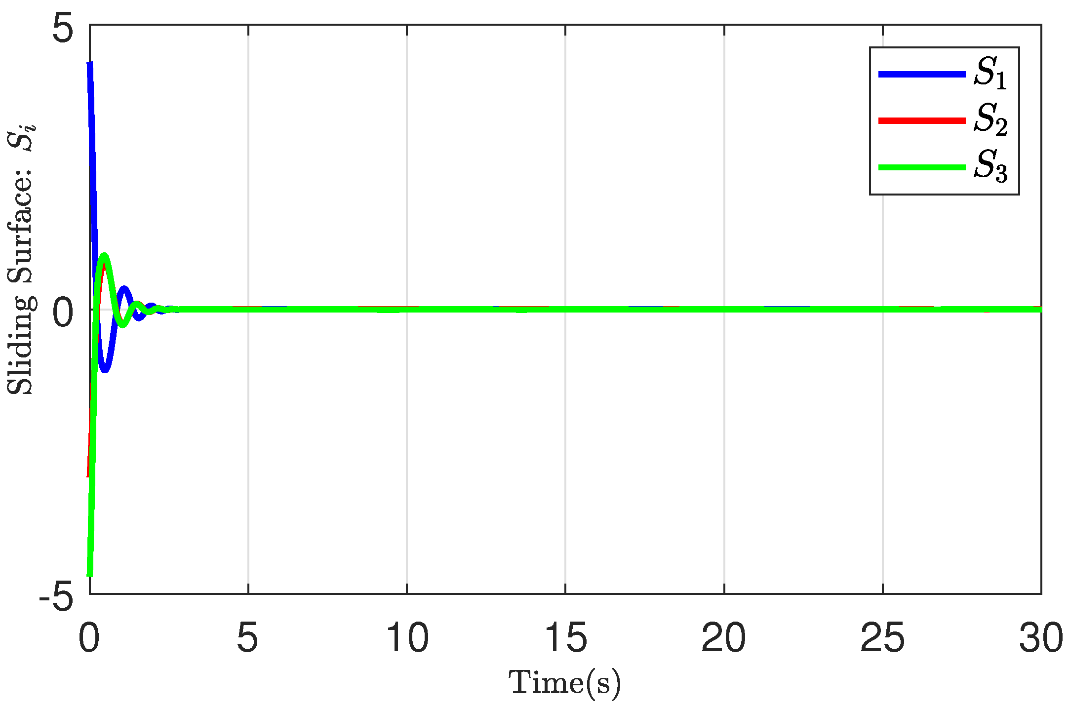
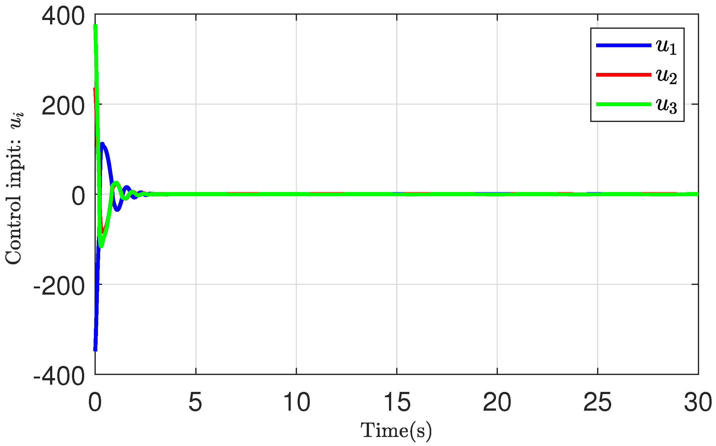
4.1. Attitude-Tracking Performance

In this subsection, the effectiveness of controller (35) is investigated for attitude stabilization. In the process of designing controller (35), these parameters are set as ${\mu }_l={\mu }_h=0.8$, $\tau =100I_3$, $p=q=0.6$, ${\sigma }_1\left(t\right)={\sigma }_2\left(t\right)=e^{-0.1t}$, $K_a=0.2I_3$, ${ϵ}_0=1$, ${ϵ}_1=1$, $\widehat{\theta }\left(0\right)=0.1$, and $\widehat{\eta }\left(0\right)=0.1$. For the novel FTPF, the parameters are chosen as ${\beta }_n=2$ and ${\beta }_{T_r}=0.05$, $T_r=10$.

Simulation results are shown in Figure 2, Figure 3, Figure 4 and Figure 5. The attitude-tracking error $q_e$ and the preselected boundary are illustrated in Figure 2. The angular velocity tracking error ${\Omega }_e$ is illustrated in Figure 3. Despite the unknown external disturbance and an uncertain inertial matrix existing, the designed robust adaptive SMC controller still achieves a good tracking convergence for the spacecraft system. The attitude-tracking error $q_e$ is the finite-time convergence from Figure 2, which means the attitude of spacecraft q can track the desired attitude $q_d$ in finite time. Meanwhile, the angular velocity tracking error ${\Omega }_e$ is also the finite-time convergence from Figure 3. The trajectory of the sliding surface is given in Figure 4. Although the sliding surface inevitably produces the chattering, the designed sliding surface is smooth, and there are few chatterings from Figure 4. The control input is depicted in Figure 5. The curve has no great fluctuation, and the convergence time of controller (35) is also short according to Figure 5. These figures prove the effectiveness of the designed controller (35).

From the above simulation results in Figure 2, Figure 3, Figure 4 and Figure 5, it can be easily gathered that all the signals of spacecraft system are bounded and the attitude-tracking error $q_e$ can converge to a preselected adjustable range in prescribed time. Thus, the attitude-tracking control target is achieved by the numerical simulations.

Remark 7.

Due to the parameter values of ${\mu }_0$ and μ being relatively large, the controller has a big jump in the beginning of time.

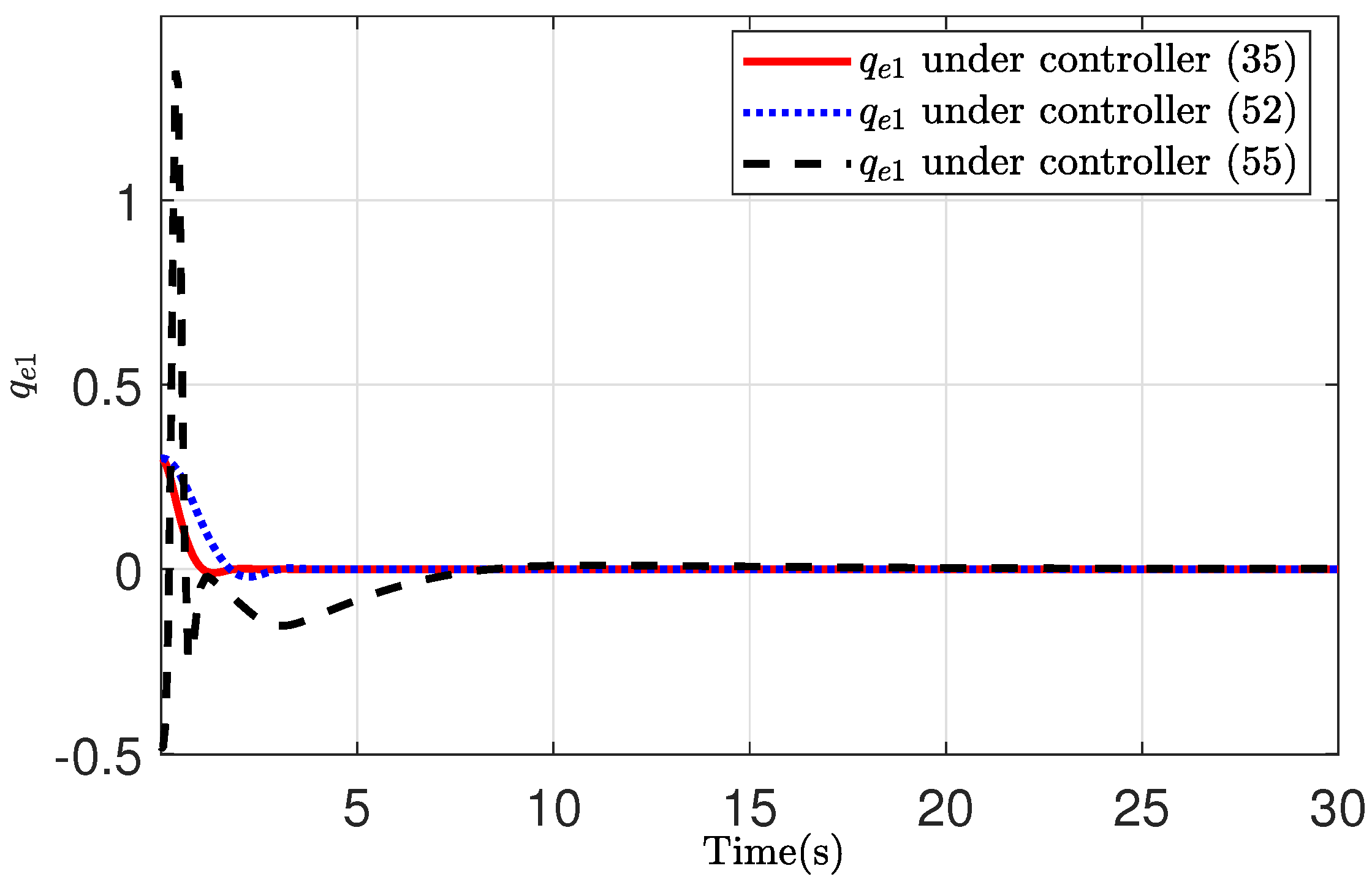
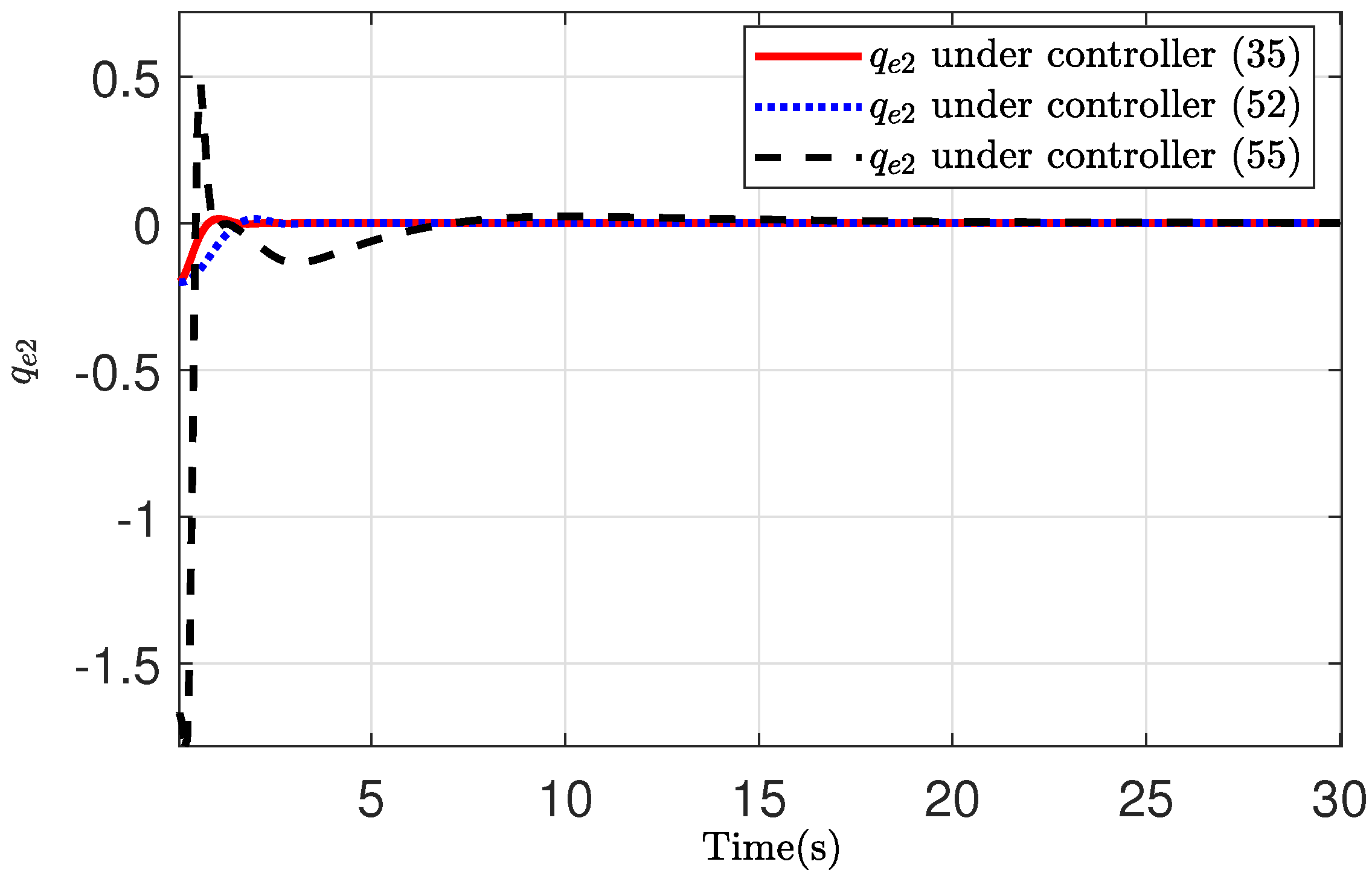
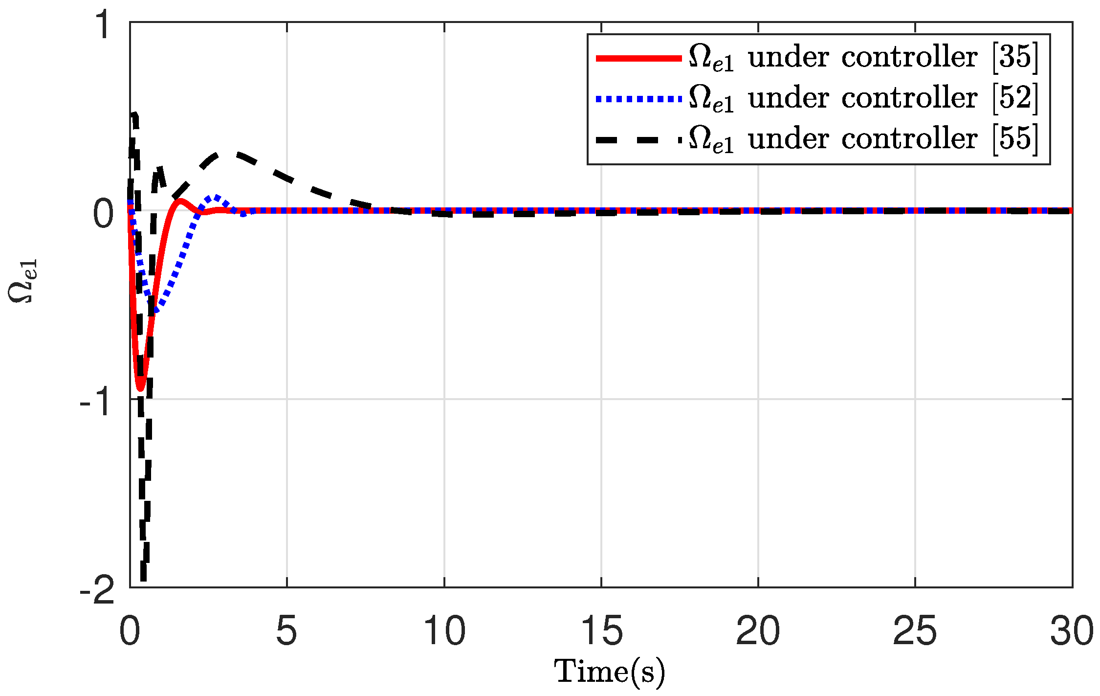
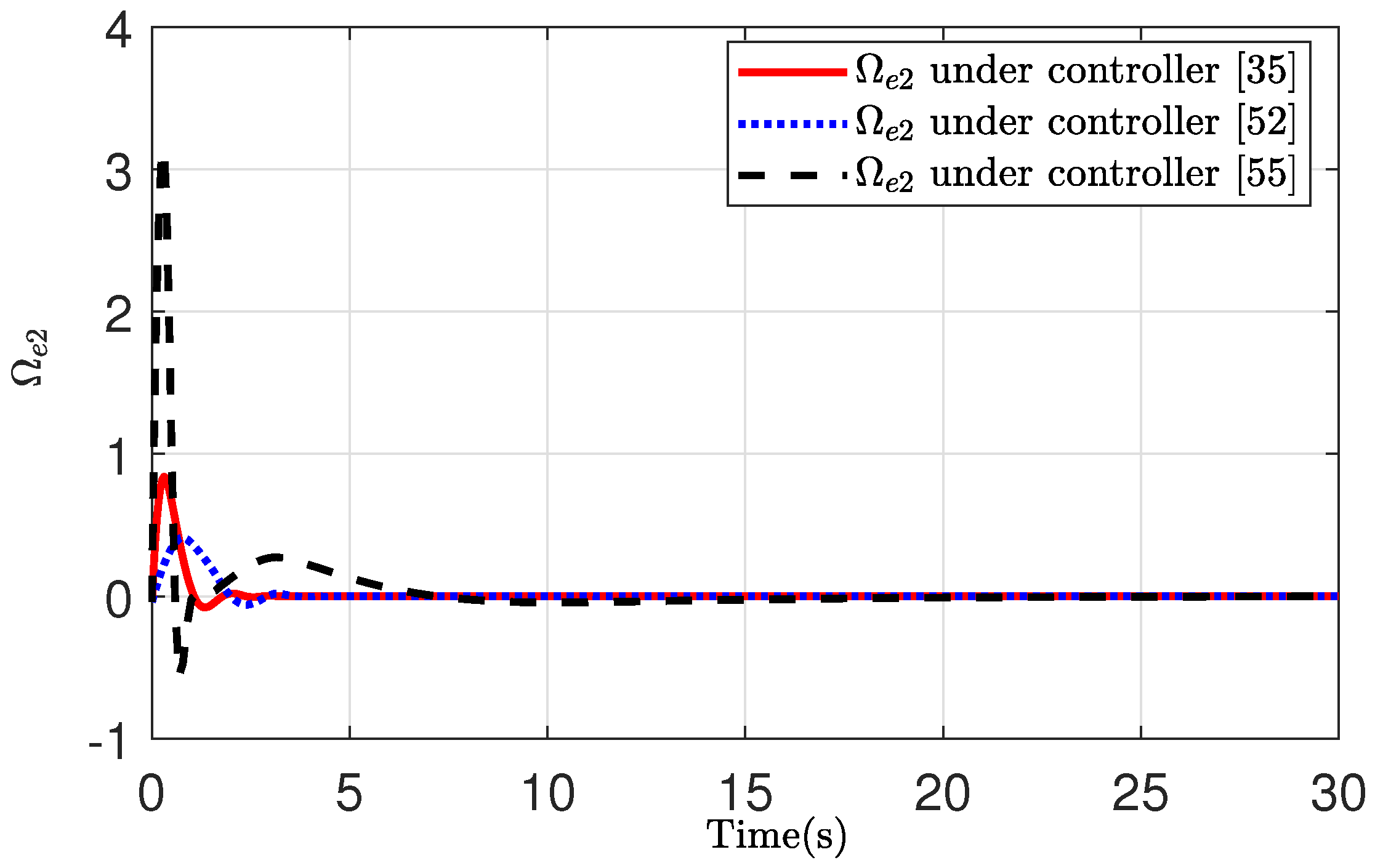
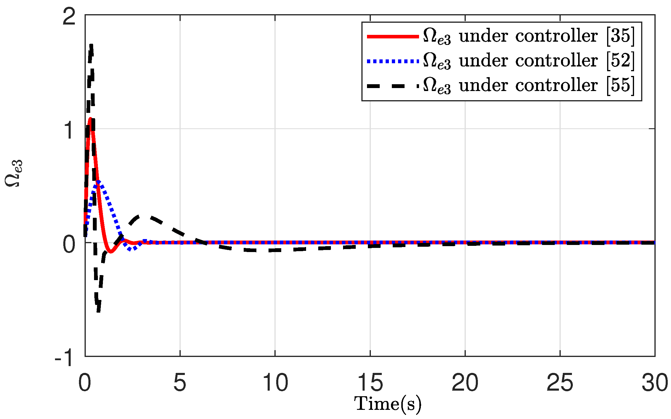
4.2. Comparative Simulations

In this subsection, some comparative simulations are given to illustrate the superiority of the controller (35). The controller (52) and the controller (55) are adopted to make a fair comparison. For a fair comparison to the performance of controllers, the initial states of system, J and d, are the same.

(i) A fast nonsingular terminal sliding mode surface (FNTSMS) in [42] is designed as $S_2={\Omega }_e+k_1{q}_e+k_2{S}_{ou}$ with $k_1=k_2=1$ and $S_{ou}$ being designed as:

$$S_{ou}=\left\{\begin{array}{cc}{q}_{ei}^r,\hfill & \hfill if{\overline{S}}_i=0or{\overline{S}}_i\ne 0,\left|q_{ei}\right|\ge \epsilon \\ l_1{q}_{ei}+l_{2}sgn\left(q_{ei}\right)q_{ei}^2,\hfill & \hfill if{\overline{S}}_i\ne 0,\left|q_{ei}\right|<\epsilon \end{array}\right.$$

(52)

where ${\overline{S}}_i={\Omega }_{ei}+k_1{q}_{ei}+k_2{q}_{ei}^r$, $r=0.6$, and $\epsilon =0.001$.

The corresponding finite-time controller in [42] is designed as follows:

$$\begin{array}{c}\hfill u_2\left(t\right)=-{\tau }_2{S}_2-{\rho }_{2}sig{n}^{\gamma }\left(S_2\right)-u_{adp}\left(t\right)\end{array}$$

(53)

where ${\tau }_2=20I_3$, ${\rho }_2=10I_3$, $\gamma =0.5$. The adaptive law $u_{adp}\left(t\right)$ is designed as:

$$u_{adp}\left(t\right)=\left\{\begin{array}{cc}\frac{S_{2i}}{|S_{2i}|}{\widehat{\zeta }}_i,\hfill & \hfill if|S_{2i}\left(t\right)|\widehat{\zeta }>{ϵ}_i\\ \frac{S_{2i}}{{ϵ}_i}{\widehat{\zeta }}_i^2,\hfill & \hfill if|S_{2i}\left(t\right)|\widehat{\zeta }\le {ϵ}_i\end{array}\right.$$

(54)

where ${\widehat{\zeta }}_i={\widehat{h}}_i+{\widehat{v}}_i\parallel \kappa \parallel$, $\parallel \kappa \parallel =max\{\parallel \Omega \parallel ,\parallel \Omega {\parallel }^2\}$, ${\dot{\widehat{h}}}_i=-a_{1i}{\widehat{h}}_i+{\overline{p}}_i\left|S_{2i}\right|$, and ${\dot{\widehat{v}}}_i=-a_{2i}{\widehat{v}}_i+{\overline{q}}_i|S_{2i}|\parallel \kappa \parallel$ are the adaptive control algorithms and $a_{1i}=a_{2i}=0.35$, ${\overline{p}}_i={\overline{q}}_i=6$.

(ii) A robust adaptive SCM controller without the PPC is designed by using the backstepping method. The sliding surface is chosen as $S_1={\Omega }_e+K{q}_e$ with $K=2I_3$, and the finite-time controller is designed as:

$$\begin{array}{c}\hfill u_1\left(t\right)=-{\tau }_1{S}_1-{\rho }_{1}sig{n}^r\left(S_1\right)-\frac{1}{2}{q}_e-\frac{S_1^T}{S_1}\widehat{\xi }\end{array}$$

(55)

where $\widehat{\xi }={\mu }_0\widehat{m}+\widehat{n}$. The adaptive control algorithms are designed as:

$$\begin{array}{c}\hfill \dot{\widehat{m}}\left(t\right)=p_1(-{\sigma }_3\widehat{m}+{\mu }_0\parallel S_1\left(t\right)\parallel )\dot{\widehat{n}}\left(t\right)=q_1(-{\sigma }_4\widehat{n}+\parallel S_1\left(t\right)\parallel )\end{array}$$

(56)

where ${\mu }_0={\parallel \Omega \parallel }^2+\parallel {\Omega }_e^{\times }C{\Omega }_d\parallel +\parallel C{\dot{\Omega }}_d\parallel$. ${\tau }_1={\rho }_1=100I_3$, $r=0.8$, and $p_1=q_1=0.6$ are the designed parameters. ${\sigma }_3\left(t\right)={\sigma }_4\left(t\right)=e^{-0.1t}$. $\widehat{m}\left(0\right)=1$ and $\widehat{n}\left(0\right)=1$ denote the initial value.

The comparison of simulation results is collected in Figure 6, Figure 7, Figure 8, Figure 9, Figure 10 and Figure 11. Figure 6, Figure 7 and Figure 8 give the trajectory of attitude-tracking errors $q_{ei}$ under controller (35), (52), and (55), respectively. Figure 9, Figure 10 and Figure 11 give the trajectory of angular velocity tracking errors ${\Omega }_{ei}$ under controller (35), (52), and (55), respectively. It can be seen from Figure 6, Figure 7, Figure 8, Figure 9, Figure 10 and Figure 11 that $q_{ei}\left(t\right)$ and ${\Omega }_{ei}\left(t\right)$ all achieve the finite-time convergence. Comparing controller (35) with controllers (52) and (55), the convergence time of tracking errors is the shortest by using controller (35). In addition,

Table 1. The steady-state attitude-tracking errors $q_{ei}$ under controller (35), (52), and (55), respectively.

Steady-State Tracking Errors ${\mathit{q}}_{\mathbf{ei}}$	Under (35)	Under (52)	Under (55)
$q_{e1}$	$1.29\times {10}^{-7}$	$-3.53\times {10}^{-5}$	$0.83\times {10}^{-3}$
$q_{e2}$	$3.55\times {10}^{-7}$	$-0.13\times {10}^{-3}$	$0.11\times {10}^{-2}$
$q_{e3}$	$-2.65\times {10}^{-7}$	$2.69\times {10}^{-5}$	$0.70\times {10}^{-3}$

and

Table 2. The steady-state angular velocity tracking errors ${\Omega }_{ei}$ under controller (35), (52), and (55), respectively.

Steady-State Tracking Errors ${\mathbf{\Omega }}_{\mathbf{ei}}$	Under (35)	Under (52)	Under (55)
${\Omega }_{e1}$	$-1.75\times {10}^{-6}$	$-6.67\times {10}^{-5}$	$-0.36\times {10}^{-2}$
${\Omega }_{e2}$	$-1.88\times {10}^{-6}$	$-9.77\times {10}^{-5}$	$-0.44\times {10}^{-3}$
${\Omega }_{e3}$	$-1.41\times {10}^{-6}$	$-0.20\times {10}^{-3}$	$-0.29\times {10}^{-2}$

list the data of steady-state tracking errors. It can be found that the value of steady-state tracking errors is the smallest by using controller (35).

From Figure 6, Figure 7, Figure 8, Figure 9, Figure 10 and Figure 11, the convergence rate is slow, and the larger chattering is generated for the tracking errors under controller (55). Due to the poor convergence of tracking errors under controller (55), the comparison of convergence is emphasized for the tracking errors under controller (52) and controller (55). Under controller (52), a small amplitude is produced in the initial stage, but the convergence time is slower. Under controller (35), the convergence rate of tracking errors is faster. From Table 1 and Table 2, the steady-state tracking errors are minimum under controller (35), and the steady-state tracking errors are maximal under controller (55). From the above simulation results, the convergence rate and accuracy of tracking errors are better under controller (35). Thus, the superiority of controller (35) is verified.

At the same time, the proposed control scheme in this article has an advantage that the time can be prescribed in advance, which can be better applied to practical space tasks. By adjusting parameters, the following conclusions can be obtained: (1) If the prescribed time $T_r$ is decreased, the convergence rate is faster, but a larger chattering is generated and the steady-state accuracy is reduced. (2) If the preselected range is decreased, the control input chatters violently. Therefore, ${\mu }_l$, ${\mu }_h$, and the prescribed time $T_r$ should be prudently chosen to balance the convergence time and steady-state accuracy. The parameters of the controller (35) are chosen by a trial-by-trial selection to ensure better convergence.

5. Conclusions

In this article, the problem of finite-time attitude-tracking control for the spacecraft system with the external disturbance and an uncertain inertial matrix has been studied. Firstly, by using the sliding mode control (SMC) technology and the boundary estimation method, the state trajectory of system can be completely driven to the sliding surface. Then, the designed robust adaptive controller ensures that the attitude-tracking error of the spacecraft converges to a preselected boundary in the prescribed time. What is more, by using the first-order sliding mode differentiator (FOSD), the problem of “explosion of complexity” has been solved, which was caused by the traditional backstepping method. Finally, the numerical simulations prove that the proposed control scheme can deal well with the finite-time attitude-tracking control problem of the spacecraft system.

The future work of this article includes the following two parts. Firstly, it is assumed that the angular velocity and derivative are bounded in this article. The adaptive control method [43] can be improved in future research projects to eliminate this assumption. Secondly, the current prescribed performance control(PPC) method is only applied to the single-spacecraft system. Recently, the concept of multispacecraft systems has been proposed in [26,35]. A research topic in the future will be the application of the PPC to the multispacecraft systems.

References

1. Wang, M.; Chen, B.; Liu, X. Adaptive fuzzy tracking control for a class of perturbed strict-feedback nonlinear time-delay systems. Fuzzy. Sets. Syst. 2008, 159, 949–967. [Google Scholar] [CrossRef]
2. Zuo, Z.; Tie, L. Distributed robust finite-time nonlinear consensus protocols for multi-agent systems. Int. J. Syst. Sci. 2016, 47, 1366–1375. [Google Scholar] [CrossRef]
3. Du, H.; Li, S.; Qian, C. Finite-time attitude-tracking control of spacecraft with application to attitude synchronization. IEEE Trans. Automat. Contr. 2011, 56, 2711–2717. [Google Scholar] [CrossRef]
4. Xia, Y.; Zhu, Z.; Wang, S. Attitude-tracking of rigid spacecraft with bounded disturbances. IEEE Trans. Ind. Electron. 2010, 58, 647–659. [Google Scholar] [CrossRef]
5. Niu, B.; Zhao, J. Tracking control for output-constrained nonlinear switched systems with a barrier Lyapunov function. Int. J. Syst. Sci. 2013, 44, 978–985. [Google Scholar] [CrossRef]
6. Xiao, B.; Shen, Y.; Wu, L. A structure simple controller for satellite attitude-tracking maneuver. IEEE Trans. Ind. Electron. 2016, 64, 1436–1446. [Google Scholar] [CrossRef]
7. Lee, T. Robust Adaptive attitude-tracking on SO(3) with an application to a quadrotor UAV. IEEE Trans. Control Syst. Technol. 2012, 21, 1924–1930. [Google Scholar]
8. Zou, L.; Wang, Z.D.; Han, Q.L. Tracking Control Under Round-Robin Scheduling: Handling Impulsive Transmission Outliers. IEEE Trans. Cybern. 2021. [Google Scholar] [CrossRef]
9. Luo, W.; Chu, Y.; Ling, K. Inverse optimal adaptive control for attitude-tracking of spacecraft. IEEE. Trans. Automat. Contr. 2005, 50, 1639–1654. [Google Scholar]
10. Chen, Z.; Jie, H. Attitude-tracking and disturbance rejection of rigid spacecraft by adaptive control. IEEE Trans. Automat. Contr. 2009, 54, 600–605. [Google Scholar] [CrossRef]
11. Wang, M.; Chen, B.; Zhang, S. Adaptive neural tracking control of nonlinear timedelay systems with disturbances. Int. J. Adapt. Control Signal. Process. 2009, 23, 1031–1049. [Google Scholar] [CrossRef]
12. Sun, L.; Zheng, Z. Saturated adaptive hierarchical fuzzy attitude-tracking control of rigid spacecraft with modeling and measurement uncertainties. IEEE Trans. Ind. Electron. 2018, 66, 3742–3751. [Google Scholar] [CrossRef]
13. Zou, A.M.; Krishna, D.K. Adaptive fuzzy fault-tolerant attitude control of spacecraft. Control Eng. Pract. 2011, 19, 10–21. [Google Scholar] [CrossRef]
14. Liu, Y.; Yang, G.H.; Li, X.J. Fault-tolerant control for uncertain linear systems via adaptive and LMI approaches. Int. J. Syst. Sci. 2017, 48, 347–356. [Google Scholar] [CrossRef]
15. Sari, N.N.; Jahanshahi, H.; Fakoor, M. Adaptive fuzzy PID controlstrategy for spacecraft attitude control. Int. J. Fuzzy. Syst. Control 2019, 21, 769–781. [Google Scholar] [CrossRef]
16. Hu, Q.; Wang, Z.D.; Gao, H. Sliding mode and shaped input vibration control of flexible systems. IEEE Trans. Aerosp. Electron. Syst. 2008, 44, 503–519. [Google Scholar]
17. Niu, Y.; Ho, D.; Wang, Z.D. Improved sliding mode control for discrete-time systems via reaching law. IET. Control Theory Appl. 2010, 4, 2245–2251. [Google Scholar] [CrossRef]
18. Hu, J.; Wang, Z.D.; Gao, H. Robust sliding mode control for discrete stochastic systems with mixed time delays, randomly occurring uncertainties, and randomly occurring nonlinearities. IEEE Trans. Ind. Electron. 2011, 59, 3008–3015. [Google Scholar] [CrossRef] [Green Version]
19. Qiang, S.; Wang, D.W.; Zhu, S.Q. Inertia-free fault-tolerant spacecraft attitude-tracking using control allocation. Automatica 2015, 62, 114–121. [Google Scholar]
20. Gu, X.; Jia, T.; Niu, Y. Consensus tracking for multi-agent systems subject to channel fading: A sliding mode control method. Int. J. Syst. Sci. 2020, 51, 2703–2711. [Google Scholar] [CrossRef]
21. Vadali, S.R. Variable-structure control of spacecraft large-angle maneuvers. J. Guid. Control Dyn. 1986, 9, 235–239. [Google Scholar] [CrossRef]
22. Pukdeboon, C.; Zinober, A.S. Quasi-continuous higher order sliding-mode controllers for spacecraft attitude-tracking maneuvers. IEEE Trans. Ind. Electron. 2009, 57, 1436–1444. [Google Scholar] [CrossRef] [Green Version]
23. Huo, B.Y.; Xia, Y.Q. Attitude stabilization of rigid spacecraft with finite-time convergence. Int. J. Robust Nonlinear Control 2011, 21, 686–702. [Google Scholar]
24. Huo, B.Y.; Xia, Y.Q.; Lu, K.F. Adaptive fuzzy finite-time fault-tolerant attitude control of rigid spacecraft. J. Franklin. Inst. 2015, 352, 4225–4246. [Google Scholar] [CrossRef]
25. Huo, B.Y.; Xia, Y.Q.; Yin, L. Fuzzy adaptive fault-tolerant output feedback attitude-tracking control of rigid spacecraft. IEEE Trans. Syst. Man Cybern. Syst. 2016, 47, 1898–1908. [Google Scholar] [CrossRef]
26. Zhao, L.; Jia, Y. Neural network-based adaptive consensus tracking control for multi-agent systems under actuator faults. Int. J. Syst. Sci. 2016, 47, 1931–1942. [Google Scholar] [CrossRef]
27. Xing, L.; Zhang, J. Fuzzy logic based adaptive event triggered sliding mode control for spacecraft attitude tracking. Aerosp. Sci. Technol. 2021, 108, 106394. [Google Scholar] [CrossRef]
28. Zou, A.M. Finite-time attitude-tracking control for spacecraft using terminal sliding mode and Chebyshev neural network. IEEE Trans. Syst. Man Cybern. Syst. 2011, 41, 950–963. [Google Scholar]
29. Cui, B.; Xia, Y.Q.; Liu, K. Truly Distributed Finite-Time Attitude Formation-Containment Control for Networked Uncertain Rigid Spacecraft. IEEE Trans. Cybern. 2020. [Google Scholar] [CrossRef]
30. Bechlioulis, C.P.; Rovithakis, G.A. Prescribed performance adaptive control of SISO feedback linearizable systems with disturbances. In Proceedings of the 16th Mediterranean Conference on Control and Automation, Ajaccio, France, 25–27 June 2008; pp. 1035–1040. [Google Scholar]
31. Bechlioulis, C.P.; Rovithakis, G.A. Robust adaptive control of feedback linearizable MIMO nonlinear systems with prescribed performance. IEEE Trans. Automat. Contr. 2008, 53, 2090–2099. [Google Scholar] [CrossRef]
32. Wang, M.; Ye, H.; Chen, Z. Neural learning control of flexible joint manipulator with predefined tracking performance and application to baxter robot. Complexity 2017, 2017, 1–14. [Google Scholar] [CrossRef]
33. Wang, M.; Yang, A. Dynamic learning from adaptive neural control of robot manipulators with prescribed performance. IEEE Trans. Syst. Man Cybern. Syst. 2017, 47, 2244–2255. [Google Scholar] [CrossRef]
34. Liu, Y.; Liu, X.P.; Jing, Y.W. Adaptive neural networks finite-time tracking control for non-strict feedback systems via prescribed performance. Inf. Sci. 2018, 468, 29–46. [Google Scholar] [CrossRef]
35. Wei, C.; Luo, J.; Dai, H. Learning-based adaptive attitude control of spacecraft formation with guaranteed prescribed performance. IEEE Trans. Cybern. 2018, 49, 4004–4016. [Google Scholar] [CrossRef] [PubMed]
36. Jing, Y.W.; Liu, Y.; Zhou, S.W. Prescribed performance finite-time tracking control for uncertain nonlinear systems. J. Syst. Sci. Complex. 2019, 32, 803–817. [Google Scholar] [CrossRef]
37. Gao, S.; Liu, X.; Jing, Y.; Dimirovski, G.M. A novel finite-time prescribed performance control scheme for spacecraft attitude-tracking. Aerosp. Sci. Technol. 2021, 118, 107044. [Google Scholar] [CrossRef]
38. Levant, A. Robust exact differentiation via sliding mode technique. Automatica 1998, 34, 379–384. [Google Scholar] [CrossRef]
39. Khalil, H.K. Nonlinear Systems, 3rd ed.; Patience Hall: Hoboken, NJ, USA, 2002. [Google Scholar]
40. Hu, Q.; Shao, X.; Guo, L. Adaptive fault-tolerant attitude tracking control of spacecraft with prescribed performance. IEEE ASME Trans. Mechatron. 2017, 23, 331–341. [Google Scholar] [CrossRef]
41. Tao, J.W.; Tao, Z.; Liu, Q.R. Novel finite-time adaptive neural control of flexible spacecraft with actuator constraints and prescribed attitude-tracking performance. Acta Astronaut. 2021, 179, 646–658. [Google Scholar] [CrossRef]
42. Lu, K.; Xia, Y. Adaptive attitude tracking control for rigid spacecraft with finite-time convergence. Automatica 2013, 49, 3591–3599. [Google Scholar] [CrossRef]
43. Hu, Q.; Shao, X. Smooth finite-time fault-tolerant attitude tracking control for rigid spacecraft. Aerospace Sci. Technol. 2016, 55, 144–157. [Google Scholar] [CrossRef]
Figure 1. The comparison of novel FTPF β ( t ) and conventional FTPF β o l d ( t ) . Different colors of curves represent different performance functions.
Mathematics 10 00401 g001
Figure 2. The attitude-tracking errors under controller (35): q e i , i = 1 , 2 , 3 and the preselected upper boundary μ h β ( t ) and the preselected lower boundary μ l β ( t ) under constraint (4). Different colors represent different components of the attitude-tracking error.
Mathematics 10 00401 g002
Figure 3. The angular velocity tracking errors under controller (35): Ω e i , i = 1 , 2 , 3 . Different colors represent different components of the attitude-tracking error.
Mathematics 10 00401 g003
Figure 4. The sliding surface under controller (35): S i , i = 1 , 2 , 3 . Different colors represent different components of the sliding surface.
Mathematics 10 00401 g004
Figure 5. The control input under controller’ (35): u i , i = 1 , 2 , 3 . u 1 , u 2 . Different colors represent different components of the control input.
Mathematics 10 00401 g005
Figure 6. The first component of the attitude-tracking error: q e 1 . Three different curves represent the attitude-tracking error under controller (35), (52), and (55), respectively.
Mathematics 10 00401 g006
Figure 7. The second component of the attitude-tracking error: q e 2 . Three different curves represent the attitude-tracking error under controller (35), (52), and (55), respectively.
Mathematics 10 00401 g007
Figure 8. The third component of the attitude-tracking error: q e 3 . Three different curves represent the attitude-tracking error under controller (35), (52), and (55), respectively.
Mathematics 10 00401 g008
Figure 9. The first component of the angular velocity tracking error: Ω e 1 . Three different curves represent the angular velocity tracking error under controller (35), (52), and (55), respectively.
Mathematics 10 00401 g009
Figure 10. The second component of the angular velocity tracking error: Ω e 2 . Three different curves represent the angular velocity tracking error under controller (35), (52), and (55), respectively.
Mathematics 10 00401 g010
Figure 11. The third component of the angular velocity tracking error: Ω e 3 . Three different curves represent the angular velocity tracking error under controller (35), (52), and (55), respectively.
Mathematics 10 00401 g011