
Stochastic Analysis of Nonlinear Cancer Disease Model through Virotherapy and Computational Methods


Abstract
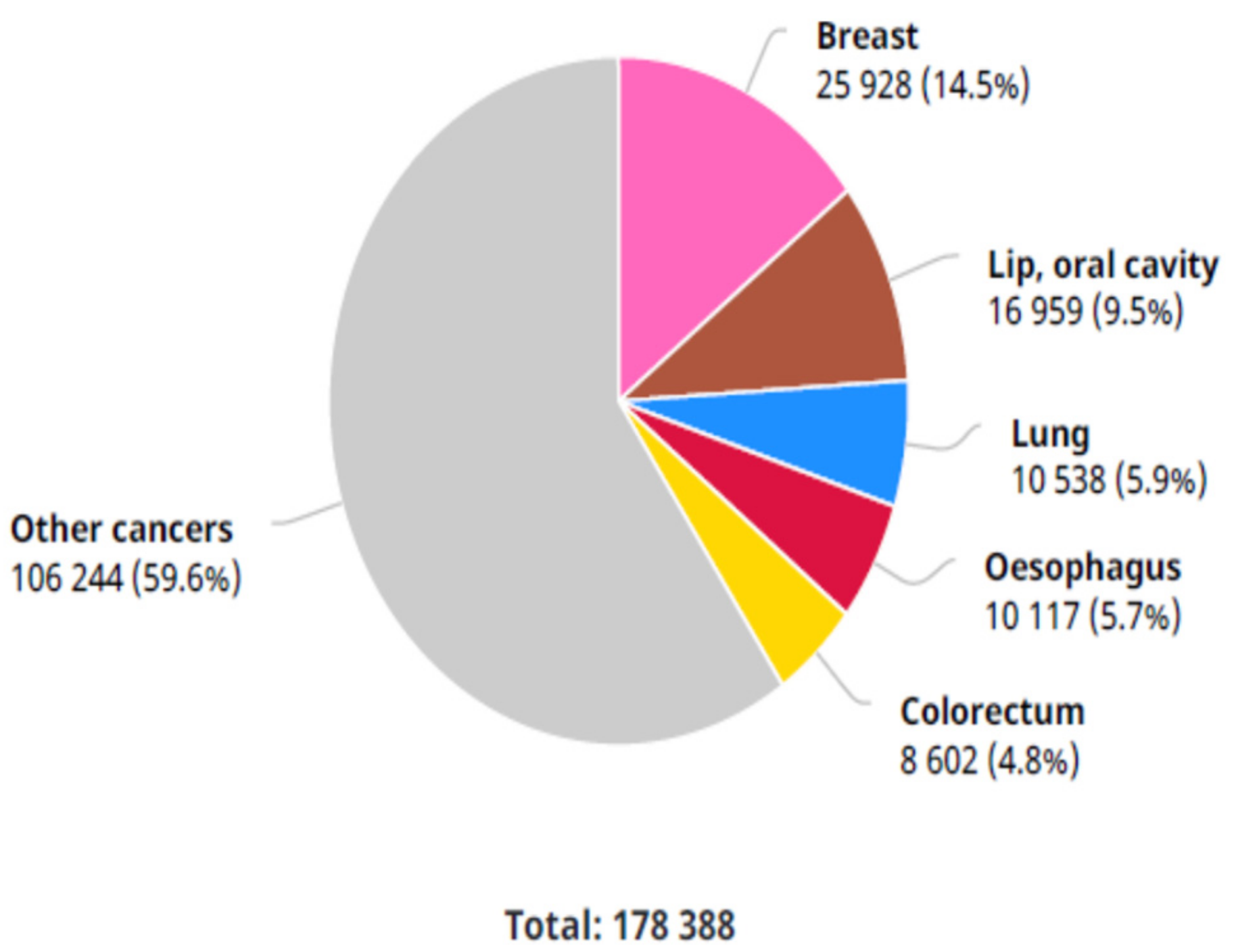
:1. Introduction
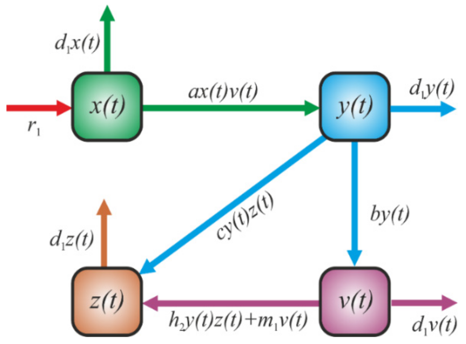
2. Deterministic Formulation
2.1. Analysis of Model
2.2. Reproduction Number
2.3. Local Stability
3. Stochastic Cancer Virotherapy Model
3.1. Euler Maruyama Method
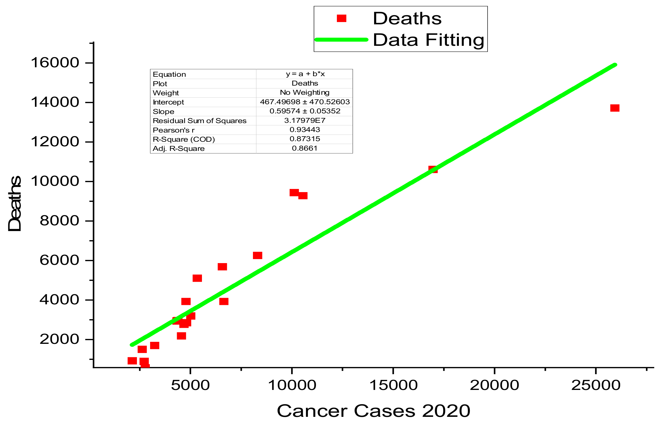
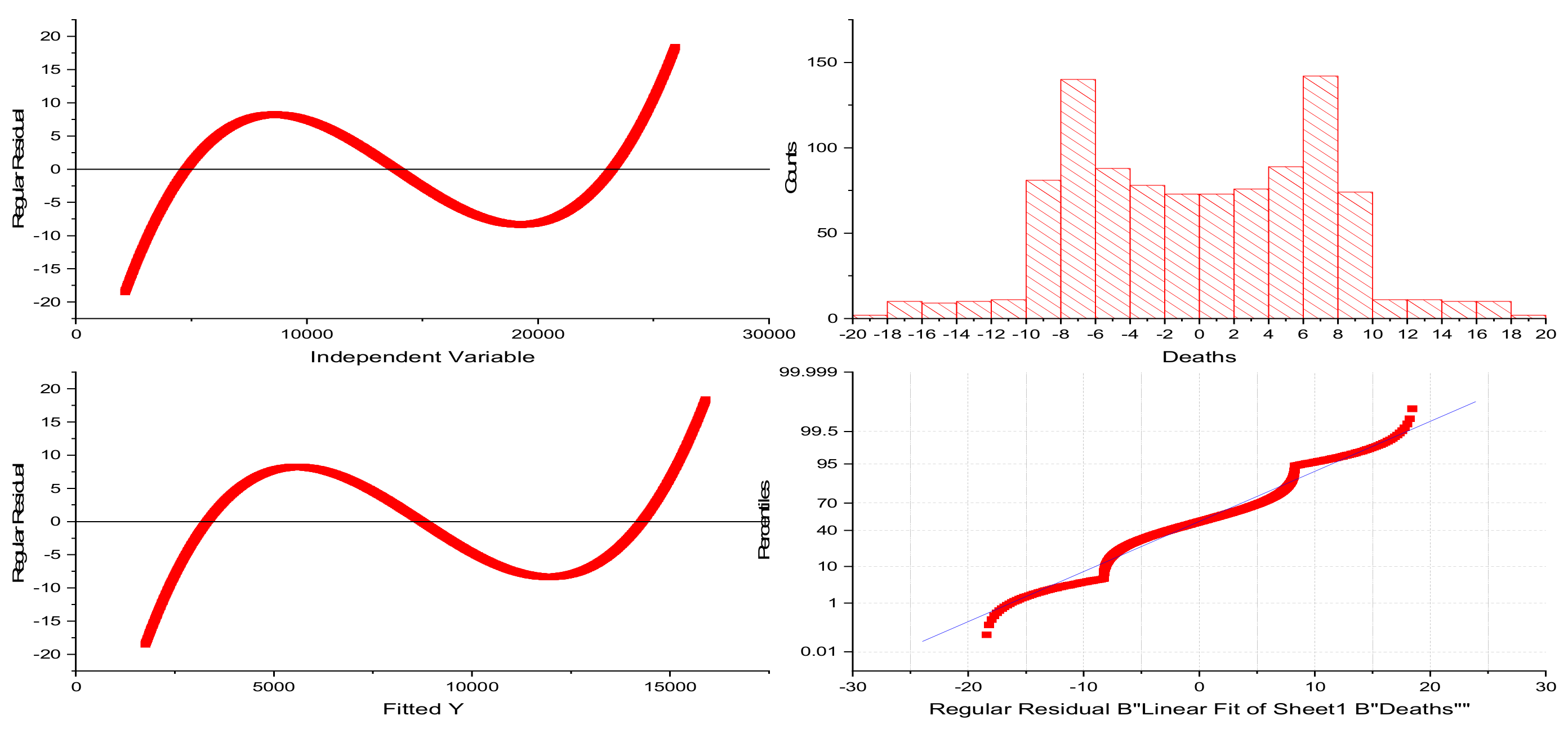
3.2. Data Curation
3.3. Non-Parametric Perturbation of Model
3.4. Positivity and Boundedness of Stochastic Model
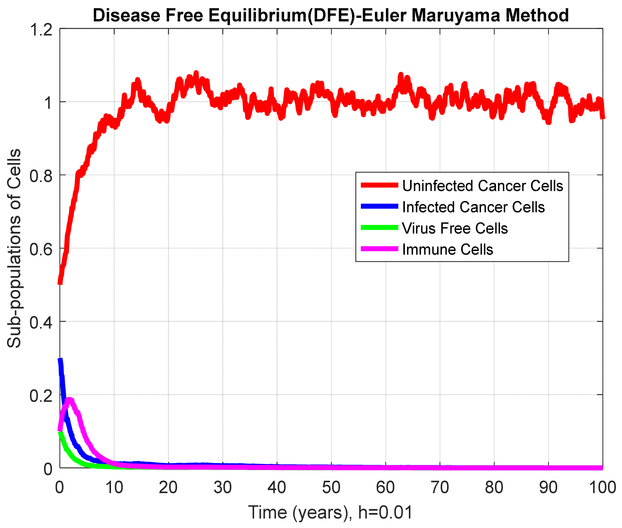
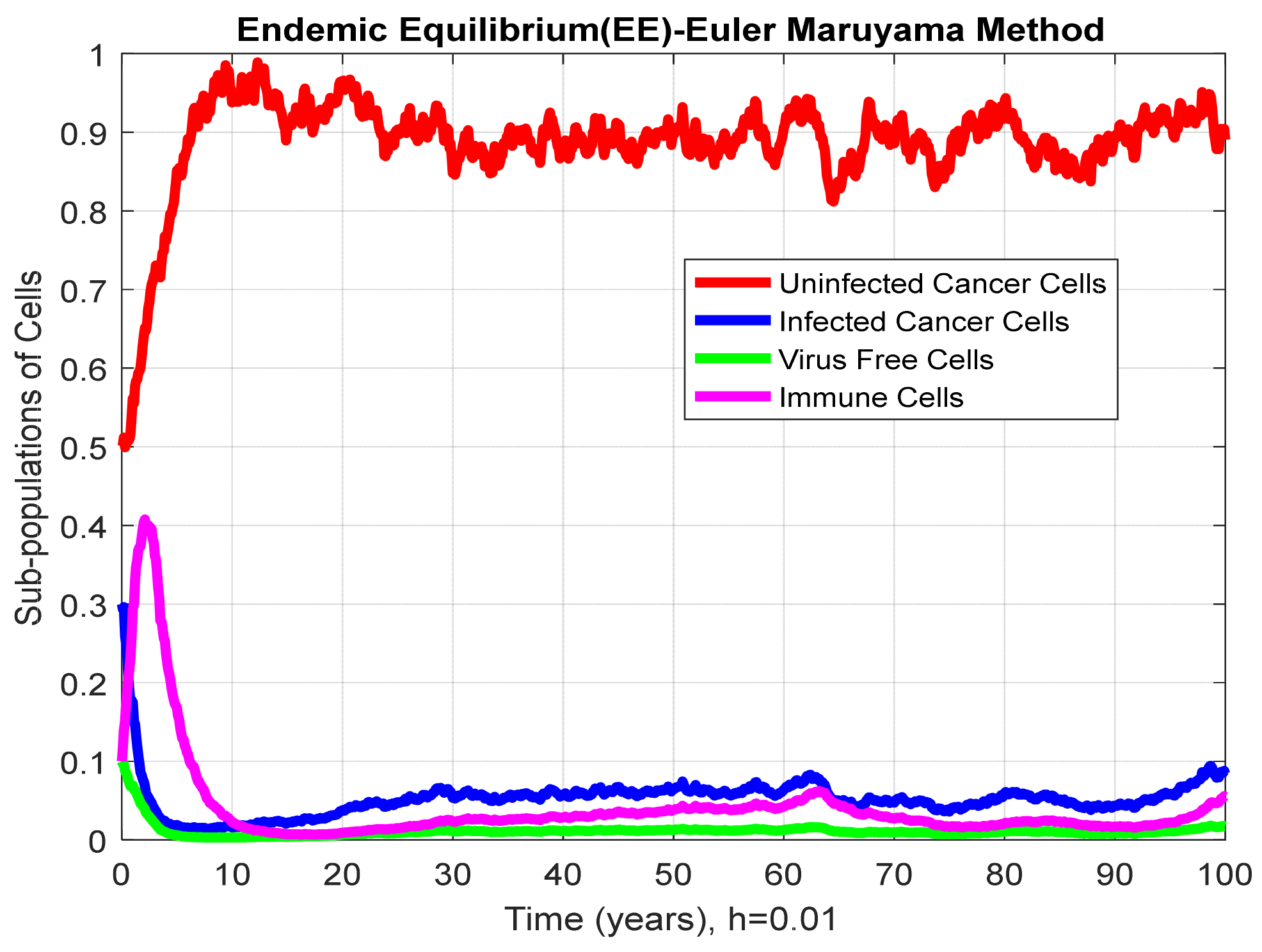
4. Computational Methods
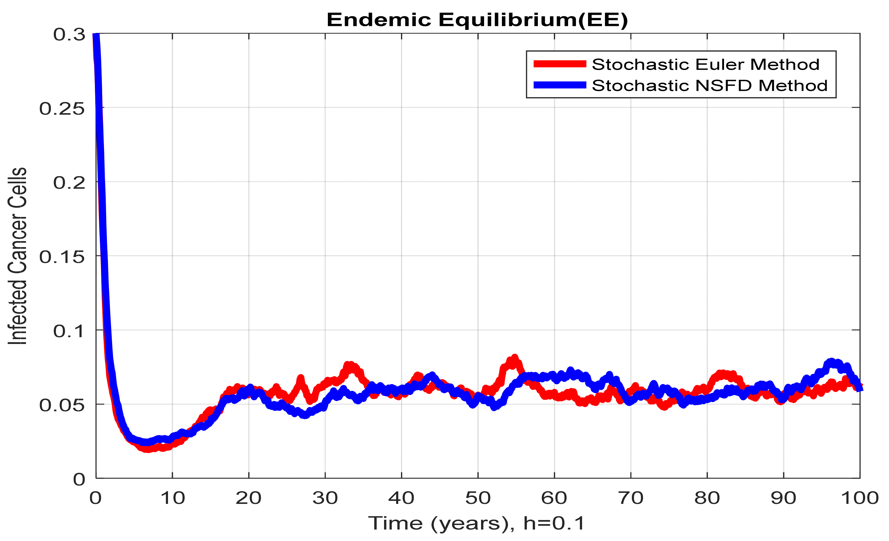
4.1. Stochastic Euler
4.2. Stochastic Runge Kutta
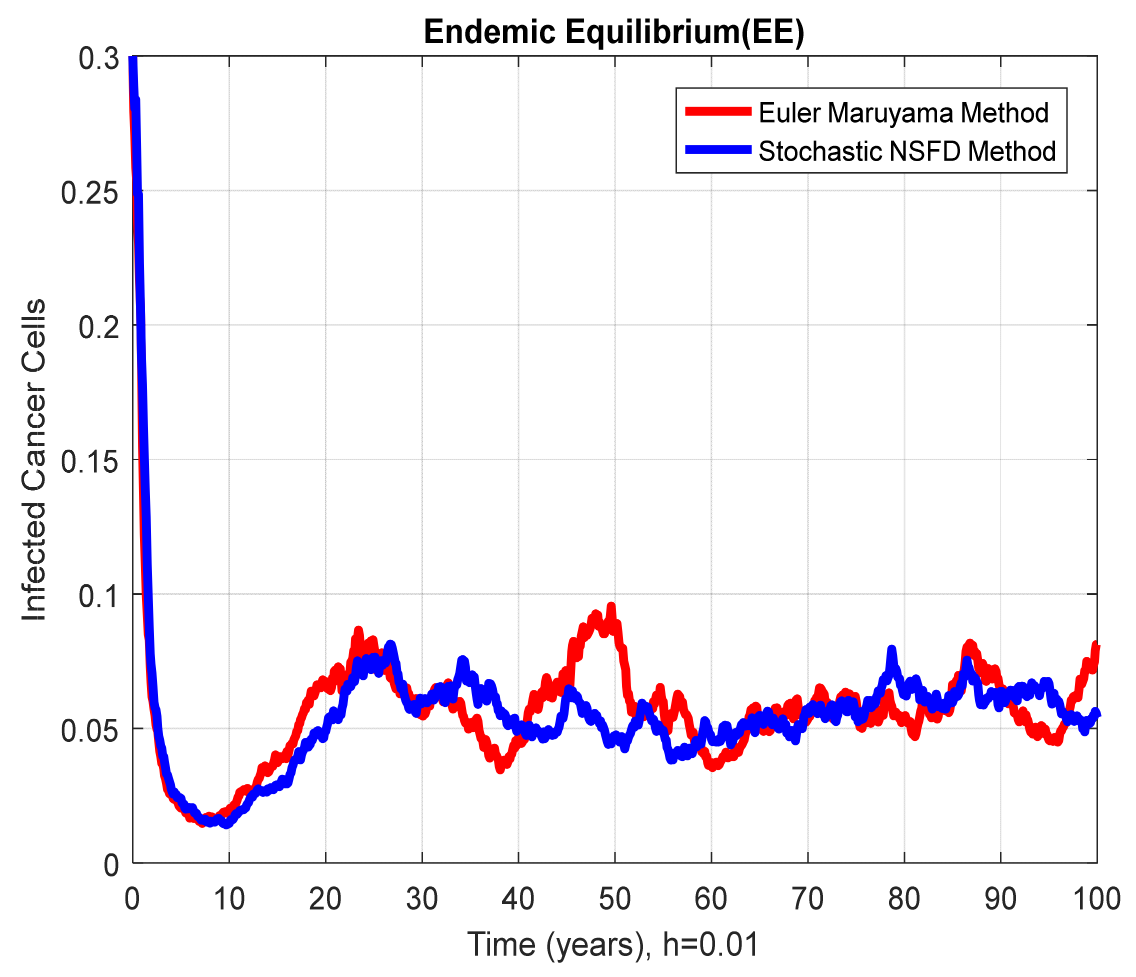
4.3. Stochastic NSFD
4.4. Stability Analysis
- (i)
- .
- (ii)
- .
- (iii)
- .
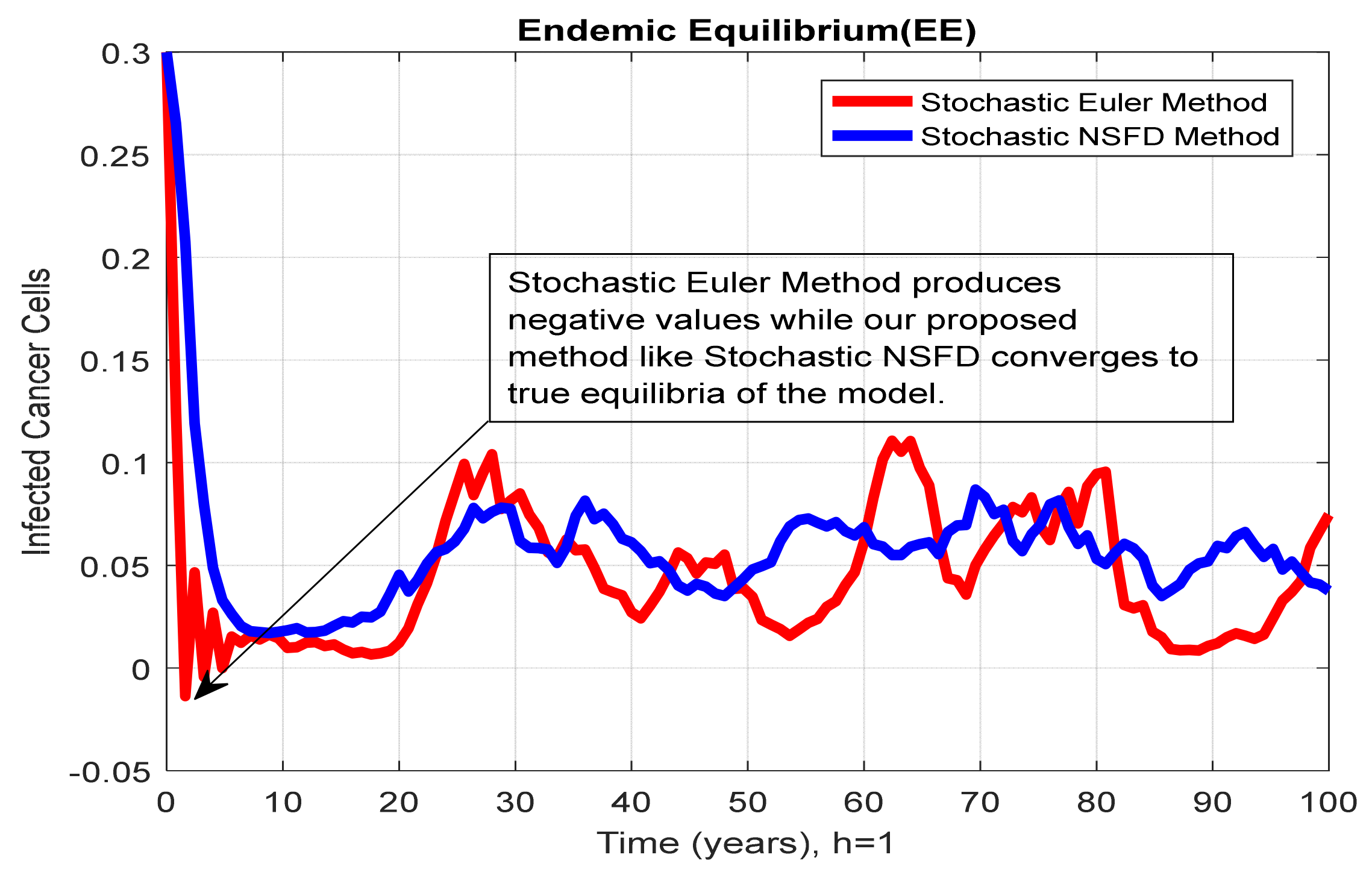
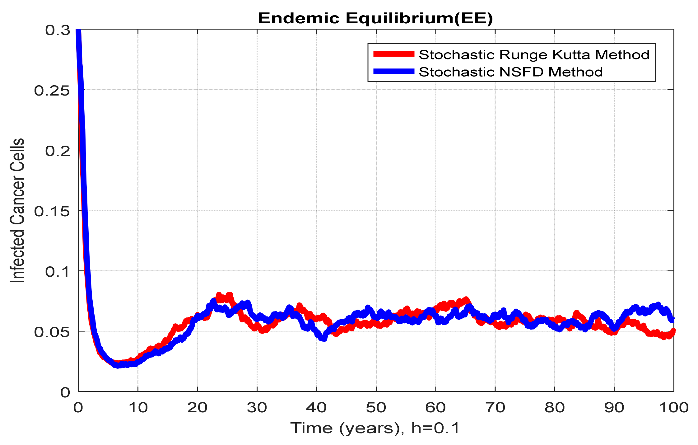
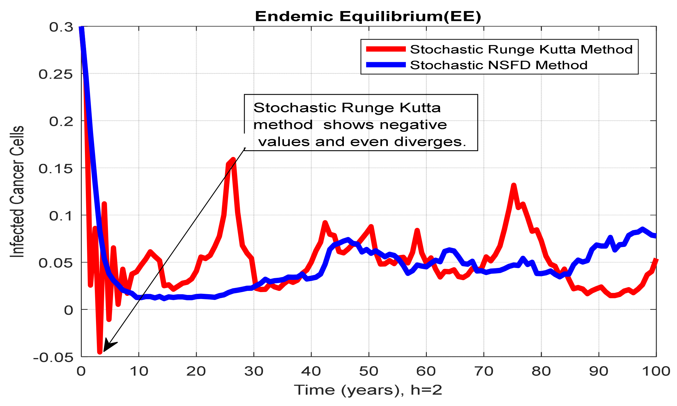
4.5. Comparison Section
5. Conclusions
Author Contributions
Funding
Data Availability Statement
Acknowledgments
Conflicts of Interest
Appendix A
Appendix B
Appendix C
Appendix D
References
- Tuwairqi, A.; Johani, O.N.A.; Simbawa, A.E. Modeling Dynamics of Cancer Virotherapy with Immune Response. Adv. Differ. Equ. 2020, 438, 1–26. [Google Scholar]
- Crivelli, J.J.; Földes, J.; Kim, P.; Wares, J.R. A mathematical model for cell cycle-specific cancer virotherapy. J. Biol. Dyn. 2012, 6, 104–120. [Google Scholar] [CrossRef] [PubMed] [Green Version]
- Nouni, A.; Hattaf, K.; Yousfi, N. Dynamics of a Virological Model for Cancer Therapy with Innate Immune Response. Complexity 2020, 2020, 8694821. [Google Scholar] [CrossRef]
- Storey, K.M.; Lawler, S.E.; Jackson, T.L. Modeling Oncolytic Viral Therapy, Immune Checkpoint Inhibition, and the Complex Dynamics of Innate and Adaptive Immunity in Glioblastoma Treatment. Front. Physiol. 2020, 11, 151. [Google Scholar] [CrossRef] [PubMed]
- Abernathy, Z.; Abernathy, K.; Stevens, J. A mathematical model for tumor growth and treatment using virotherapy. AIMS Math. 2020, 5, 4136–4150. [Google Scholar] [CrossRef]
- Matos, L.A.; Franco, S.L.; McFadden, G. Oncolytic Viruses and the Immune System: The Dynamic Duo. Mol. Theory 2020, 4, 349–358. [Google Scholar]
- Makaryan, S.Z.; Cess, C.G.; Finley, S.D. Modeling immune cell behavior across scales in cancer. Wiley Interdiscip. Rev. Syst. Biol. Med. 2020, 12, e1484. [Google Scholar] [CrossRef] [Green Version]
- Malinzi, J.; Eladdadi, A.; Sibanda, P. Modelling the spatiotemporal dynamics of chemovirotherapy cancer treatment. J. Biol. Dyn. 2017, 11, 244–274. [Google Scholar] [CrossRef] [Green Version]
- Bajzer, Ž.; Carr, T.; Josić, K.; Russell, S.J.; Dingli, D. Modeling of cancer virotherapy with recombinant measles viruses. J. Theor. Biol. 2008, 252, 109–122. [Google Scholar] [CrossRef]
- Timalsina, S.; Tian, J.P.; Wang, J. Mathematical and Computational Modeling for Tumor Virotherapy with Mediated Immunity. Bull. Math. Biol. 2017, 79, 1736–1758. [Google Scholar] [CrossRef]
- Rommelfanger, D.M.; Offord, C.P.; Dev, J.; Bajzer, Z.; Vile, R.G.; Dingli, D. Dynamics of Melanoma Tumor Therapy with Vesicular Stomatitis Virus: Explaining the Variability in Outcomes Using Mathematical Modeling. Gene Ther. 2012, 19, 543–549. [Google Scholar] [CrossRef] [PubMed] [Green Version]
- Liu, X.; Li, Q.; Pan, J. A deterministic and stochastic model for the system dynamics of tumor–immune responses to chemotherapy. Phys. A Stat. Mech. Its Appl. 2018, 500, 162–176. [Google Scholar] [CrossRef] [Green Version]
- Eftimie, R.; Eftimie, G. Tumour-associated Macrophages and Oncolytic Virotherapies: A mathematical investigation into a complex-dynamics. Lett. Biomath. 2018, 5, S6–S35. [Google Scholar] [CrossRef]
- Santiago, D.N.; Heidbuechel, J.P.W.; Kandell, W.M.; Walker, R.; Djeu, J.; Engeland, C.E.; Abate-Daga, D.; Enderling, H. Fighting Cancer with Mathematics and Viruses. Viruses 2017, 9, 239. [Google Scholar] [CrossRef] [PubMed] [Green Version]
- Kim, S.P.; Lee, P.P. Modeling protective anti-tumor immunity via preventative cancer vaccines using a hybrid agent-based and delay differential equation approach. PLoS Comput. Biol. 2012, 8, e1002742. [Google Scholar] [CrossRef] [Green Version]
- Berg, D.R.; Offord, C.P.; Kemler, I.; Ennis, M.K.; Chang, L.; Paulik, G.; Bajzer, Z.; Neuhauser, C.; Dingli, D. In vitro and in silico multidimensional modeling of oncolytic tumor virotherapy dynamics. PLoS Comput. Biol. 2019, 15, e1006773. [Google Scholar] [CrossRef] [Green Version]
- International Agency for Research on Cancer. Available online: https://gco.iarc.fr/today/data/factsheets/populations/586-pakistan-fact-sheets.pdf (accessed on 1 March 2021).
- Ijaz, M.F.; Attique, M.; Son, Y. Data-driven cervical cancer prediction model with outlier detection and over-sampling methods. Sensors 2020, 20, 2809. [Google Scholar] [CrossRef]
- Ijaz, M.F.; Alfian, G.; Syafrudin, M.; Rhee, J. Hybrid prediction model for type-2 diabetes and hypertension using DBSCAN-based outlier detection, synthetic minority over-sampling technique (SMOTE), and random forest. Appl. Sci. 2018, 8, 1325. [Google Scholar] [CrossRef] [Green Version]
- Mandal, M.; Singh, P.K.; Ijaz, M.F.; Shafi, J.; Sarkar, R. A tri-stage wrapper-filter feature selection framework for disease classification. Sensors 2021, 21, 5571. [Google Scholar] [CrossRef]
- Panigrahi, R.; Borah, S.; Bhoi, A.K.; Ijaz, M.F.; Pramanik, M.; Kumar, Y.; Jhaveri, R.H. A consolidated decision tree-based intrusion detection system for binary and multiclass imbalanced datasets. Mathematics 2021, 9, 751. [Google Scholar] [CrossRef]
- Panigrahi, R.; Borah, S.; Bhoi, A.K.; Ijaz, M.F.; Pramanik, M.; Jhaveri, R.H.; Chowdhary, C.L. Performance assessment of supervised classifiers for designing intrusion detection systems: A comprehensive review and recommendations for future research. Mathematics 2021, 9, 690. [Google Scholar] [CrossRef]
- Srinivasu, P.N.; SivaSai, J.G.; Ijaz, M.F.; Bhoi, A.K.; Kim, W.; Kang, J.J. Classification of skin disease using deep learning neural networks with mobile net V2 and LSTM. Sensors 2021, 21, 2852. [Google Scholar] [CrossRef] [PubMed]
- Arif, M.S.; Raza, A.; Rafiq, M.; Bibi, M.; Abbasi, J.N.; Nazeer, A.; Javed, U. Numerical Simulations for Stochastic Computer Virus Propagation Model. Comput. Mater. Contin. 2020, 62, 61–77. [Google Scholar] [CrossRef]
- Shatanawi, W.; Arif, M.S.; Raza, A.; Rafiq, M.; Bibi, M.; Abbasi, J.N. Structure-Preserving Dynamics of Stochastic Epidemic Model with the Saturated Incidence Rate. Comput. Mater. Contin. 2020, 64, 797–811. [Google Scholar] [CrossRef]
- Bayram, M.; Partal, T.; Buyukoz, G.O. Numerical methods for simulation of stochastic differential equations. Adv. Differ. Equ. 2018, 2018, 17. [Google Scholar] [CrossRef] [Green Version]
- Abukhaled, M.I.; Allen, E.J. A class of second-order Runge-Kutta methods for numerical solution of stochastic differential equations. Stoch. Anal. Appl. 1998, 16, 977–991. [Google Scholar] [CrossRef]
- Abukhaled, M.; Allen, E.J. A recursive integration method for approximate solution of stochastic differential equations. Int. J. Comput. Math. 1998, 66, 53–66. [Google Scholar] [CrossRef]
- Sghir, A.; Hadiri, S. A new numerical method for 1-D backward stochastic differential equations without using conditional expectations. Random Oper. Stoch. Equ. 2020, 28, 79–91. [Google Scholar] [CrossRef]
- Halidias, N. A novel approach to construct numerical methods for stochastic differential equations. Numer. Algorithm 2013, 66, 79–87. [Google Scholar] [CrossRef] [Green Version]
- Higham, D.J.; Mao, X.; Szpruch, L. Convergence, non-negativity and stability of a new Milstein scheme with applications to finance. arXiv 2012. Available online: https://scholar.google.com/scholar?hl=en&as_sdt=0%2C5&q=Convergence%2C+non-negativity+and+stability+of+a+new+Milstein+scheme+with+applications+to+finance&btnG= (accessed on 1 March 2021).
- Rebiha, Z. New numerical method for solving nonlinear stochastic integral equations. Владикавказский Математический Журнал 2020, 22. Available online: https://scholar.google.com/scholar?hl=en&as_sdt=0%2C5&q=New+numerical+method+for+solving+nonlinear+stochastic+integral+equations&btnG= (accessed on 1 March 2021).
- Słomiński, L. Stability of strong solutions of stochastic differential equations. Stoch. Process. Their Appl. 1989, 31, 173–202. [Google Scholar] [CrossRef] [Green Version]
- Abukhaled, M.I. Mean square stability of second-order weak numerical methods for stochastic differential equations. Appl. Numer. Math. 2004, 48, 127–134. [Google Scholar] [CrossRef]


| Parameters | Values |
|---|---|
| 0.5 | |
| a | 5.1 (EE) 3.1 (DFE) |
| 0.63 | |
| 0.5 | |
| C | 5.048 (EE) 3.048(DFE) |
| b | 0.22 |
| 0.016 | |
| 0.6 | |
Publisher’s Note: MDPI stays neutral with regard to jurisdictional claims in published maps and institutional affiliations. |
© 2022 by the authors. Licensee MDPI, Basel, Switzerland. This article is an open access article distributed under the terms and conditions of the Creative Commons Attribution (CC BY) license (https://creativecommons.org/licenses/by/4.0/).
Share and Cite
Raza, A.; Awrejcewicz, J.; Rafiq, M.; Ahmed, N.; Mohsin, M. Stochastic Analysis of Nonlinear Cancer Disease Model through Virotherapy and Computational Methods. Mathematics 2022, 10, 368. https://doi.org/10.3390/math10030368
Raza A, Awrejcewicz J, Rafiq M, Ahmed N, Mohsin M. Stochastic Analysis of Nonlinear Cancer Disease Model through Virotherapy and Computational Methods. Mathematics. 2022; 10(3):368. https://doi.org/10.3390/math10030368
Chicago/Turabian StyleRaza, Ali, Jan Awrejcewicz, Muhammad Rafiq, Nauman Ahmed, and Muhammad Mohsin. 2022. "Stochastic Analysis of Nonlinear Cancer Disease Model through Virotherapy and Computational Methods" Mathematics 10, no. 3: 368. https://doi.org/10.3390/math10030368