An Enhanced Grey Wolf Optimizer with a Velocity-Aided Global Search Mechanism

Abstract

This paper proposes a novel variant of the Grey Wolf Optimization (GWO) algorithm, named Velocity-Aided Grey Wolf Optimizer (VAGWO). The original GWO lacks a velocity term in its position-updating procedure, and this is the main factor weakening the exploration capability of this algorithm. In VAGWO, this term is carefully set and incorporated into the updating formula of the GWO. Furthermore, both the exploration and exploitation capabilities of the GWO are enhanced in VAGWO via stressing the enlargement of steps that each leading wolf takes towards the others in the early iterations while stressing the reduction in these steps when approaching the later iterations. The VAGWO is compared with a set of popular and newly proposed meta-heuristic optimization algorithms through its implementation on a set of 13 high-dimensional shifted standard benchmark functions as well as 10 complex composition functions derived from the CEC2017 test suite and three engineering problems. The complexity of the proposed algorithm is also evaluated against the original GWO. The results indicate that the VAGWO is a computationally efficient algorithm, generating highly accurate results when employed to optimize high-dimensional and complex problems.

1. Introduction

Computational intelligence [1] is a sub-branch of artificial intelligence which employs a variety of mechanisms to solve complex problems in different domains. Computational intelligence is applied to many fields, such as computer vision, healthcare, fog computing, and others. The swarm intelligence (SI) algorithm is one of the most popular computational intelligence methods, mimicking the lifestyle of natural communities such as animal herds. The algorithms included in the SI focus on the individual lives of the swarms’ members, on the one hand, and the social relations and interactions among the swarms’ individuals to chase and find the food sources on the other. In the last few years, many SI algorithms have been developed and proposed, including the Firefly Algorithm (FA) [2], Cuckoo Search (CS) [3], Grey Wolf Optimizer (GWO) [4], Moth-Flame Optimization (MFO) [5], Gradient-Based Optimizer (GBO) [6], Whale Optimization Algorithm (WOA) [7], Arithmetic Optimization Algorithm (AOA) [8], and Aquila Optimizer (AO) [9].

In the same context, Grey Wolf Optimizer (GWO) is one of the most popular and widely used SI-based techniques [4]. The GWO algorithm is inspired by the behavior of the grey wolves in nature when seeking the best means for hunting prey. The GWO algorithm applies the same mechanism and follows the pack hierarchy for assigning different roles to each member of the pack to reach the food depending on its potential fitness and its rank in the pack. In GWO, four groups of wolves, including alpha, beta, delta, and omega wolves, are defined based upon the highest fitness to leadership to the lowest competence, respectively. As the alpha, beta, and delta wolves are rated as the guide wolves in GWO, the omega wolves always follow the location of these guides when searching for food in nature. The GWO is started by generating random positions for the grey wolves. Then, the three high-fitness wolves are assumed as those with the best locations in the population and are named the alpha, beta, and delta solutions, and the other wolves’ positions are updated according to their distance from the leading solutions to bring about the potentially better agents to be determined within the searching process. The GWO employs effective operators to conduct the search process such that a safe and reliable exploration–exploitation balance could be maintained to avoid premature convergence [10].

As with a wide range of other meta-heuristic algorithms, the GWO suffers from poor performance in global search [11]. The updating equation of the GWO conducts the convergence of the algorithm very well but causes premature convergence as a result of not having a strong ability to diversify the search agents to accomplish the exploration phase. The performance of the GWO could be exacerbated when facing the high-dimensional problems, having numerous local optima [12]. To achieve a good balance between maintaining the diversity and providing a high rate of convergence in GWO, there are several GWO variants that have been proposed in recent years, which can generally be placed into four categories:

• Modification of the value of the parameters a and C. A non-linearly decreasing strategy of a was proposed in [13]. This method employs an exponential decay function by lapse of iterations. A logarithmic decay function was also proposed to modify the conventional formulation of a in [12]. The control parameter a was also dynamically adapted using fuzzy logic in [14].
• Hybridization with other strong population-based methods. In this way, the weaknesses of the GWO are covered by the strengths of several other algorithms, such as genetic algorithms [15], particle swarm optimization [16], differential evolution [17,18,19,20], and biogeography-based optimizer [21]. The integration of the GWO with some local search methods is another idea accomplished in [22,23,24].
• Modification of the updating procedure. The main motivation of this category of the GWO variants is to increase the diversity of the GWO population to enable this algorithm to better perform the exploration phase of the optimization process. Among the proposed variants in this category, the exploration enhanced GWO (EEGWO) is aimed at adding a selected random search agent from the population to the conventional leading alpha, beta, and delta agents to guide the other individuals in the population [25]. A weighted distance GWO (wdGWO) was also proposed in [26]. This variant uses a weighted average of the best individuals instead of the simple average. Inspired by PSO, a new updating scheme replacing the alpha, beta, and delta positions with the positions of the personal historical best position of a solution (Pbest) and the global best position (Gbest) was also proposed in [12].
• Employment of the new operators. A cellular GWO (CGWO) utilizing a topological structure was developed in [27]. In this method, each wolf merely interacts with its neighbors in an attempt to make the search process more local to inject more diversity into the population. A fuzzy hierarchical operator, a mutation operator, and a Lévy flight operator accompanied by a greedy selection strategy were employed to enhance the exploration capability of the GWO in [28,29,30], respectively. A random walk operator was also suggested for use in GWO in a new variant of GWO named RW-GWO [31]. Recently, a refraction learning operator was suggested to help the alpha wolf not to be trapped in the local optimum in a new GWO variant called RL-GWO [11].

The original GWO algorithm suffers from lacking a strong and reliable exploration capability, as this algorithm only uses the acceleration terms to update the wolves. Guiding the wolves only based on the acceleration each leading wolf can apply to the others can make the global search of the wolves incomplete and thus inefficient as a result of possibly creating successive interruptions and disruptions in the path of the search agents when attempting to globally search the search space of the optimization problems. In this paper, we propose a novel variant of the GWO, named Velocity-Aided GWO (VAGWO), to effectively solve the crucial problem of the original GWO, briefly explained above. In this algorithm, a new updating procedure is proposed for the wolves, in which each wolf adopts a velocity term as well. The major contributions of this paper can be highlighted as follows:

• Since the original GWO only involves the acceleration terms to update the position of the wolves (search agents), these agents may be trapped in local optima, and thereby a large number of good solutions are not detected during the search process. As a result, a velocity term can highly improve the global search mechanism of the GWO. This is the main motivation for proposing VAGWO.
• The exploration and exploitation capabilities of the GWO are both enhanced via presenting a new formulation for the control parameter a to emphasize a in the early iterations while de-emphasizing this parameter in the later iterations.
• The control parameter C is also modified to intensify the search process in the last iterations to ameliorate the performance of the GWO in the exploitation phase. Additionally, the newly proposed calculation formulation of C is such that it is well adapted to the iterations of the optimization process to make a well-balanced exploration–exploitation transition in the VAGWO.

The organization of the remainder of this paper is as follows: Section 2 introduces the GWO algorithm and describes the modifications made to GWO to yield the proposed VAGWO algorithm. In Section 3.1, the proposed algorithm is applied to two series of high-dimensional benchmark functions and compared to other popular and widely used meta-heuristic algorithms. In Section 3.2, the proposal is compared with a set of newly proposed algorithms on the same test bed used in Section 3.1. In Section 3.3, a Wilcoxon rank-sum test is conducted to reveal the significance of the superiority of the VAGWO over its competitors when applied to the test functions. In Section 3.4 and Section 3.5, the computational complexity of the VAGWO is evaluated against the original GWO. In Section 3.6, the competence of the VAGWO in solving real-world engineering problems is evaluated. Finally, Section 4 highlights the main conclusions of this paper.

2. Materials and Methods

2.1. Original Grey Wolf Optimizer

The GWO algorithm mimics the hunting behavior and social leadership of grey wolves in nature [4]. The GWO starts the optimization process by randomly generating a swarm of wolves (initial solutions). At each iteration, the three best-fitted wolves, named alpha, beta, and delta, are identified as the leaders of the rest of the wolves, named omega wolves. Then, the omega wolves encircle the best wolves to find the most promising regions in the search space. These wolves act as the search agents seeking the optimal point of the optimization problems. Since every search agent encircles the three best agents in the search space, the arithmetic average of the updated positions of the alpha, beta, and delta wolves is finally adopted as the updated position of each search agent. This procedure may enhance the exploration capability of the algorithm, as three different leading agents are involved in guiding the other agents. The mathematical formulations used in updating the omega wolves are as follows:

$$D_{p,j}^t=\left|C_{p,j}^t\times X_{p,j}^t-X_{i,j}^t\right|$$

(1)

$$X_{i,j}^{t+1}=X_{p,j}^t-A_{p,j}^t{D}_{p,j}^t$$

(2)

where t stands for the current iteration; $A_{p,j}^t={2r}_1\times a-a$; $C_{p,j}^t={2r}_2$; $X_{p,j}^t$ is the position of the prey in the jth dimension in the tth iteration; and $X_{i,j}^t$ is the position of the ith grey wolf in the jth dimension in the tth iteration. Additionally, $r_1$ and $r_2$ are two random numbers generated in [0, 1]. Furthermore, $a$ is linearly decreased from 2 to 0, by means of the lapse of iterations. Factor $A$ maintains an exploration–exploitation balance in the algorithm. Furthermore, $C$ is also multiplied by the prey position to further help the exploration capability of the algorithm via preventing the wolves from being trapped in local optima.

Each omega wolf is updated according to the alpha, beta, and delta wolves, as formulated below:

$$D_{\alpha ,j}^t=\left|C_{\alpha ,j}^t\times X_{\alpha ,j}^t-X_{i,j}^t\right|$$

(3)

$$D_{\beta ,j}^t=\left|C_{\beta ,j}^t\times X_{\beta ,j}^t-X_{i,j}^t\right|$$

(4)

$$D_{\delta ,j}^t=\left|C_{\delta ,j}^t\times X_{\delta ,j}^t-X_{i,j}^t\right|$$

(5)

$$X_{1,j}^t=X_{\alpha ,j}^t-A_{\alpha ,j}^t\times D_{\alpha ,j}^t$$

(6)

$$X_{2,j}^t=X_{\beta ,j}^t-A_{\beta ,j}^t\times D_{\beta ,j}^t$$

(7)

$$X_{3,j}^t=X_{\delta ,j}^t-A_{\delta ,j}^t\times D_{\delta ,j}^t$$

(8)

$$X_{i,j}^{t+1}=\left(X_{1,j}^t+X_{2,j}^t+X_{3,j}^t\right)/3$$

(9)

where the subscripts $\alpha$, $\beta$, and $\delta$ denote the alpha, beta, and delta wolves. The other subscripts and superscripts are defined above. As Mirjalili et al. (2014) discussed, in GWO, half of the iterations are for exploration, when |A| > 1, and the second half is dedicated to the exploitation, in which |A| < 1.

2.2. Velocity-Aided Grey Wolf Optimizer (VAGWO)

In the original GWO, the search agents do not have velocity as a characteristic helping them in the search process. When the moving agents make their movements in the search space only by successively changing their acceleration towards the guide agents, these movements are not consistently or smoothly made iteration by iteration. In other words, a certain search agent may move towards a guiding agent in the current iteration, and when this guide changes its position, that certain agent immediately turns its trajectory to be able to move towards the new guide. As a result, a rupture may occur in the search agents’ movements in the search space, leading to potential drifts. These drifts may result in missing a large number of potentially good positions in the search space, and thereby the optimization process is doomed to face premature convergence. Considering a velocity term can help the search agents to maintain their unique trajectory, enhancing the explorative capability of the search agents, balancing the exploration and exploitation phases of the optimization process, and thus avoiding premature convergence. In VAGWO, there are initial random velocities defined for each of the search agents (wolves) when it decides to move towards each of the leading agents (alpha, beta, and delta wolves), and there are initial random positions defined for each agent (wolf) in the search space. As a result, each search agent takes a velocity and a position in each dimension of the optimization problem. Then, the agents are evaluated, and the three best-fitted agents are chosen as the alpha, beta, and delta wolves to guide the other agents (omega wolves). Then, an updating procedure is built up for the agents at each iteration. For this purpose, a velocity term is first established for the ith search agent when guided by the alpha, beta, and delta wolves, as follows:

$$V_{\alpha ,j}^{t+1}=k\times \left(\mathit{sgn}\left(A_{\alpha ,j}^t\right)\times \left|V_{\alpha ,j}^t\right|\right)+A_{\alpha ,j}^t\times D_{\alpha ,j}^t$$

(10)

$$V_{\beta ,j}^{t+1}=k\times \left(\mathit{sgn}\left(A_{\beta ,j}^t\right)\times \left|V_{\beta ,j}^t\right|\right)+A_{\beta ,j}^t{\times D}_{\beta ,j}^t$$

(11)

$$V_{\delta ,j}^{t+1}=k\times \left(\mathit{sgn}\left(A_{\delta ,j}^t\right)\times \left|V_{\delta ,j}^t\right|\right)+A_{\delta ,j}^t{\times D}_{\delta ,j}^t$$

(12)

where $V_{\alpha ,j}^t$, $V_{\beta ,j}^t$, and $V_{\delta ,j}^t$ represent the velocity of a search agent (wolf) in the jth dimension when alpha, beta, and delta wolves, respectively, are determined to attract the search agent in the updating procedure. In addition, $\mathit{sgn}$ is the sign function. $A_{\alpha ,j}^t$, $A_{\beta ,j}^t$, and $A_{\delta ,j}^t$ represent the acceleration terms of the search agents, calculated as follows:

$$A_{\alpha ,j}^t=(2\times r_1-1)\times a^2$$

(13)

$$A_{\beta ,j}^t=(2\times r_2-1)\times a^2$$

(14)

$$A_{\delta ,j}^t=(2\times r_3-1)\times a^2$$

(15)

where $r_1$, $r_2$, and $r_3$ are the uniformly distributed random numbers generated in [0, 1]. Furthermore, a is a linearly decreasing parameter successively determined as follows:

$$a=a_{\mathit{max}}-(a_{\mathit{max}}-a_{\mathit{min}})\times \left(\frac{t-1}{t_{\mathit{max}}-1}\right);a_{\mathit{max}}=\sqrt{2},a_{\mathit{min}}=0$$

(16)

As can be seen, a is changed from the value of $\sqrt{2}$ in the first iteration to the value of $0$ in the final iteration, but, according to Equations (13)–(15), the parameter a is to the power 2. This means that $a^2$ is varied from 2 to 0. The effect of the power of 2 in these equations helps the exploration and exploitation capabilities of the proposed algorithm to be strengthened. In other words, when $a^2\ge 1$, the algorithm is in the exploration phase. In addition, $a^2\ge a$, in this phase, as $a\ge 1$, and $a$ is positive. As a result, when the exploration phase is conducted by the proposed VAGWO algorithm, $a^2$ is greater than what a is expected to be in the original GWO algorithm. This means that $\left|A\right|\gg 1$, and thus the search agents are enabled to explore the search space more strongly in the exploration phase. Furthermore, when $a^2\le 1$, the algorithm is in the exploitation phase. In this phase, $a^2\le a$, as $a\le 1$, and $a$ is positive. As a result, the parameter $a^2$ is less than what a is expected to be in the original GWO algorithm, meaning that $\left|A\right|\ll 1$, and thus the exploitation phase can be more emphasized in the proposed VAGWO algorithm.

$D_{\alpha ,j}^t$, $D_{\beta ,j}^t$, and $D_{\delta ,j}^t$ denote the modified distances between a focused search agent (wolf) and the alpha, beta, and delta leading wolves, respectively. These distances in each dimension can be calculated as follows:

$$D_{\alpha ,j}^t=\left|C_{\alpha ,j}^t\times X_{\alpha ,j}^t-X_{i,j}^t\right|$$

(17)

$$D_{\beta ,j}^t=\left|C_{\beta ,j}^t\times X_{\beta ,j}^t-X_{i,j}^t\right|$$

(18)

$$D_{\delta ,j}^t=\left|C_{\delta ,j}^t\times X_{\delta ,j}^t-X_{i,j}^t\right|$$

(19)

where $X_{\alpha ,j}^t$, $X_{\beta ,j}^t$, and $X_{\delta ,j}^t$ are the positions of the alpha, beta, and delta wolves in the jth dimension in the tth iteration; $X_{i,j}^t$ is the position of the ith search agent (wolf) in the jth dimension in the tth iteration; $C_{\alpha ,j}^t$, $C_{\beta ,j}^t$, and $C_{\delta ,j}^t$ are the crucial coefficients multiplied by each leading wolf to stochastically emphasize or de-emphasize them, as there is an uncertainty in the fitness of each of the alpha, beta, and delta wolves, especially in the early iterations of the optimization process. These coefficients can take these uncertainties into account and help the exploration phase be better conducted by the algorithm. In VAGWO, a new definition is presented for these coefficients, as they can be calculated as follows:

$$C_{\alpha ,j}^t=1+(2\times r_4-1)\times c^2$$

(20)

$$C_{\beta ,j}^t=1+(2\times r_5-1)\times c^2$$

(21)

$$C_{\delta ,j}^t=1+(2\times r_6-1)\times c^2$$

(22)

where $r_4$, $r_5$, and $r_6$ are the uniformly distributed random numbers generated in [0, 1], and c is a parameter adaptively determined as follows:

$$c=c_{\mathit{max}}-(c_{\mathit{max}}-c_{\mathit{min}})\times \left(\frac{t-1}{t_{\mathit{max}}-1}\right);c_{\mathit{max}}=1, c_{\mathit{min}}=0$$

(23)

The parameter c is linearly decreasing due to the lapse of iterations. As can be seen, the coefficients C are stochastically generated in [0, 2] in the first iteration, but this range is decomposed over the course of iterations and gradually changes to [0.1, 1.9], [0.2, 1.8], …, and is terminated at [1, 1] = $\left\{1\right\}$. Additionally, the way to follow these ranges is such that the ranges’ values accelerate to reach the final range values, in which no uncertainty is considered for the fitness of the leading search agents. This is due to making the parameter c to power 2. Knowing c is within [0, 1] over the whole iterations, $c^2$ is always less than c. As a result, the coefficients C are much closer to [1, 1] = $\left\{1\right\}$ at the final iterations than those at the earlier iterations. In this way, the exploitation capability of the VAGWO algorithm can be further enhanced while the exploration is also strengthened by incorporating the velocity term into the updating procedure of the search agents.

In Equations (10)–(12), the velocity terms of $V_{\alpha ,j}^t$, $V_{\beta ,j}^t$, and $V_{\delta ,j}^t$ adopt the sign of the acceleration terms of $A_{\alpha ,j}^t$, $A_{\beta ,j}^t$, and $A_{\delta ,j}^t$. This is very important in the new velocity-incorporated updating procedure proposed in VAGWO. Otherwise, there might be a chance in conflict occurring between the velocity and the acceleration which can, in turn, disrupt the agents’ movements in the search space. In Equations (10)–(12), $k$ is a tuning parameter playing the role of the inertia weight to facilitate a suitable and reliable transition from exploration to exploitation and is calculated iteration by iteration as follows:

$$k=k_{\mathit{max}}-(k_{\mathit{max}}-k_{\mathit{min}})\times \left(\frac{t-1}{t_{\mathit{max}}-1}\right);k_{\mathit{max}}=0.9, k_{\mathit{min}}=0.4$$

(24)

Finally, the next positions of the search agents (wolves) can be updated by calculating three positions of $X_{1,j}^{t+1}$, $X_{2,j}^{t+1}$, and $X_{3,j}^{t+1}$, as follows:

$$X_{1,j}^{t+1}=X_{\alpha ,j}^t-V_{\alpha ,j}^{t+1}$$

(25)

$$X_{2,j}^{t+1}=X_{\beta ,j}^t-V_{\beta ,j}^{t+1}$$

(26)

$$X_{3,j}^{t+1}=X_{\delta ,j}^t-V_{\delta ,j}^{t+1}$$

(27)

The new position of a search agent is calculated by averaging three updated positions presented in Equations (25)–(27) as follows:

$$X_{i,j}^{t+1}=\left(X_{1,j}^{t+1}+X_{2,j}^{t+1}+X_{3,j}^{t+1}\right)/3$$

(28)

where $X_{i,j}^{t+1}$ is the position of the ith search agent (wolf) in the jth dimension in the $\left(t+1\right)$th iteration. The last modification performed in the VAGWO against the original GWO is incorporating an elitism scheme in the proposed algorithm. In this way, each agent updated at an iteration of the algorithm is compared to the best position it has experienced so far and if its objective function is better, it remains in the present form and is designated as its new best-so-far position; otherwise, the current best-so-far position replaces the updated search agent. As a result, the search agents successively become better over the course of iterations. The experiments show that equipping the proposed algorithm with the elitism mechanism can highly improve the results of the optimization offered by the proposed VAGWO algorithm. Figure 1 depicts the exploration and exploitation processes conducted by the proposed VAGWO algorithm. The flowchart of the VAGWO is also illustrated in Figure 2.

3. Results and Discussion

3.1. Comparison with Popular Meta-Heuristic Algorithms

To assess the capability of the presented VAGWO method, it is first applied to 13 popular standard benchmark functions [32,33]. These functions are broken down into two main categories: uni-modal (F1–F7), and multi-modal (F8–F13). Uni-modal benchmark functions have a single global optimum. Thus, they are suitable for assessing the effectiveness of the search process of any optimization algorithm when conducting the exploitation phase, while multi-modal benchmark functions are favoured for assessing the capability of an optimization method to explore the search space. In these benchmark functions, all the global optima are shifted so that the difficulty of solving such functions is increased, as recommended in [5,34]. For conducting a thorough investigation on the potential abilities of the proposed algorithm to solve the optimization problems, it is also applied to 10 composition functions derived from the CEC2017 test suite [35,36]. These composition functions are the combination of various shifted, rotated, and biased multimodal functions. Thus, they can challenge the proposed VAGWO algorithm’s capabilities to solve real-world and complex optimization problems to a greater extent. The optimization process implemented over these benchmark functions is of the minimization type. The number of dimensions was set to 100 for the shifted standard benchmark functions and set to 50 for the composition functions. These settings can make these test problems more challenging for the proposed algorithm and its competitors to solve such high-dimensional and thus hard-to-solve problems.

3.1.1. Parameter Setting of the Algorithms

The VAGWO algorithm presented to tackle the difficulties in the test problems offered was compared with six popular meta-heuristic algorithms, namely Moth-Flame Optimization (MFO) algorithm [5], Gravitational Search Algorithm (GSA) [37], Particle Swarm Optimization (PSO) [38], Grey Wolf Optimizer (GWO) [4], Genetic Algorithm (GA) [39], and Sine Cosine Algorithm (SCA) [34]. To perform an impartial comparison, the swarm size of all algorithms was set to 30 for the shifted uni- and multi-modal functions and set to 50 for the composition functions. In addition, a maximum of 1000 iterations for all the benchmark functions were set for all algorithms. Furthermore, the stopping criterion was assumed to be met when the maximum number of iterations had elapsed. The parameter settings of the VAGWO and the popular algorithms are presented in

Table 1. Parameter settings of the VAGWO and the popular algorithms.

Algorithm	Parameter Settings
GA	${\mathit{pr}}_{crossover}=0.9;{\mathit{pr}}_{mutation}=\frac{1}{D};D=\mathrm{number}\mathrm{of}\mathrm{dimensions}$
GSA	$\alpha =20;G_0=100$
GWO	$a=\left[2,0\right]$
SCA	$A=2$
MFO	$b=1;t=\left[-1,1\right];a\in \left[-2,-1\right]$
PSO	$c_1=c_2=2;k=\left[0.9,0.4\right]; v_{\mathit{max}}=0.1(Ub-lb)$
VAGWO	$a=\left[\sqrt{2},0\right];c=\left[1,0\right];k=\left[0.9,0.4\right];v_{\mathit{max}}=0.1(Ub-lb)$

.

The average, median, best, and standard deviation (std) are computed overall 30 runs and tabulated as the performance measures benchmarked for each algorithm in solving each problem. The final results of the methods on the uni-modal, multi-modal, and composition functions are presented in

Table 2. The results achieved by the VAGWO against the popular algorithms for the uni-modal functions at D = 100.

	Criteria	GA	GSA	GWO	SCA	MFO	PSO	VAGWO
F1	Average	$1.3145\times {10}^3$	$3.3013\times {10}^4$	2.7390 × 104	$7.7868\times {10}^4$	$5.4462\times {10}^4$	$2.3717\times {10}^3$	1.1135 × 102
	Median	$1.3491\times {10}^3$	$3.3408\times {10}^4$	$2.7923\times {10}^4$	$7.7008\times {10}^4$	$5.1517\times {10}^4$	$2.2960\times {10}^3$	4.4670 × 10−5
	Best	$6.7348\times {10}^2$	$2.5631\times {10}^4$	$2.1056\times {10}^4$	$7.2993\times {10}^4$	$1.6670\times {10}^4$	$9.9523\times {10}^2$	2.1784 × 10−5
	Std	$3.5295\times {10}^2$	$4.0589\times {10}^3$	$2.9998\times {10}^3$	$3.7570\times {10}^3$	$2.7319\times {10}^4$	$8.9039\times {10}^2$	2.9420 × 102
F2	Average	$4.4012\times {10}^1$	$1.1384\times {10}^2$	$1.4334\times {10}^2$	$8.6832\times {10}^{28}$	$2.0777\times {10}^2$	3.5007 × 101	7.0141 × 101
	Median	$3.8777\times {10}^1$	$1.0862\times {10}^2$	$1.4090\times {10}^2$	$1.8767\times {10}^{24}$	$1.9796\times {10}^1$	3.1852 × 101	$6.6105\times {10}^1$
	Best	$2.5202\times {10}^1$	$6.5112\times {10}^1$	$1.1372\times {10}^2$	$1.3806\times {10}^{19}$	$1.2845\times {10}^2$	1.8119 × 101	$1.9121\times {10}^1$
	Std	1.3266 × 101	$2.9437\times {10}^1$	$1.8008\times {10}^1$	$4.6583\times {10}^{29}$	$5.0882\times {10}^1$	$1.5105\times {10}^1$	$2.9868\times {10}^1$
F3	Average	$8.3262\times {10}^4$	$5.1905\times {10}^7$	$6.2520\times {10}^4$	$7.7757\times {10}^5$	$2.9237\times {10}^5$	$1.2787\times {10}^5$	4.2826 × 104
	Median	$8.0580\times {10}^4$	$5.0496\times {10}^7$	$6.2328\times {10}^4$	$7.9153\times {10}^5$	$2.9625\times {10}^5$	$1.2639\times {10}^5$	4.3677 × 104
	Best	$3.4050\times {10}^4$	1.7880 × 107	$4.5743\times {10}^4$	$4.5868\times {10}^5$	$2.1713\times {10}^5$	$9.2114\times {10}^4$	3.2353 × 104
	Std	$2.5412\times {10}^4$	$1.7749\times {10}^7$	$9.9509\times {10}^3$	$1.8258\times {10}^5$	$5.1406\times {10}^4$	$1.6626\times {10}^4$	5.3441 × 103
F4	Average	$5.4130\times {10}^1$	$4.1485\times {10}^1$	3.0000 × 101	$8.6843\times {10}^1$	$1.1526\times {10}^2$	$5.4811\times {10}^1$	$3.6574\times {10}^1$
	Median	$5.4759\times {10}^1$	$4.1519\times {10}^1$	3.0000 × 101	$8.6705\times {10}^1$	$1.1595\times {10}^2$	$5.4992\times {10}^1$	$3.6386\times {10}^1$
	Best	$4.3826\times {10}^1$	$3.5991\times {10}^1$	3.0000 × 101	$5.8537\times {10}^1$	$1.0147\times {10}^2$	$5.0756\times {10}^1$	$3.2179\times {10}^1$
	Std	4.6386	2.4090	9.2263 × 10−6	9.1948	4.5032	2.2497	1.9721
F5	Average	$1.0439\times {10}^7$	$2.3325\times {10}^7$	$8.8129\times {10}^7$	$3.3677\times {10}^8$	$4.6664\times {10}^8$	$3.9658\times {10}^5$	6.3034 × 102
	Median	$9.9830\times {10}^6$	$2.4397\times {10}^7$	$8.4294\times {10}^7$	$3.3991\times {10}^8$	$5.3559\times {10}^8$	$3.2805\times {10}^5$	2.4761 × 102
	Best	$4.4329\times {10}^6$	$1.2336\times {10}^7$	$5.7810\times {10}^7$	$2.9990\times {10}^8$	$8.8447\times {10}^7$	$1.2544\times {10}^5$	9.2531 × 101
	Std	$3.5737\times {10}^6$	$6.4073\times {10}^6$	$1.8251\times {10}^7$	$2.4425\times {10}^7$	$3.3994\times {10}^8$	$1.9334\times {10}^5$	7.9507 × 102
F6	Average	$4.8028\times {10}^7$	$5.4047\times {10}^7$	$4.5957\times {10}^7$	$5.0700\times {10}^7$	$4.2505\times {10}^7$	$4.4737\times {10}^7$	4.2370 × 107
	Median	$4.7976\times {10}^7$	$5.4037\times {10}^7$	$4.5964\times {10}^7$	$5.0651\times {10}^7$	4.2315 × 107	$4.4722\times {10}^7$	$4.2343\times {10}^7$
	Best	$4.7432\times {10}^7$	$5.3626\times {10}^7$	$4.5183\times {10}^7$	$5.0039\times {10}^7$	$4.2315\times {10}^7$	$4.4458\times {10}^7$	4.2273 × 107
	Std	$2.7704\times {10}^5$	$2.0128\times {10}^5$	$3.8826\times {10}^5$	$3.9522\times {10}^5$	$2.6715\times {10}^5$	$1.4424\times {10}^5$	7.3410 × 104
F7	Average	3.5762	2.8100	7.1200	$6.7364\times {10}^1$	$3.0920\times {10}^2$	5.6674	1.1901
	Median	3.5377	2.4379	7.1292	$5.5946\times {10}^1$	$2.8647\times {10}^2$	5.3252	1.1240
	Best	2.8683	1.1697	4.8209	$2.3663\times {10}^1$	$1.1090\times {10}^2$	3.2343	7.4749 × 10−1
	Std	$3.8797\times {10}^{-1}$	1.2734	$8.7771\times {10}^{-1}$	$3.6755\times {10}^1$	$1.3778\times {10}^2$	1.7540	3.1510 × 10−1

,

Table 3. The results achieved by the VAGWO against the popular algorithms for the multi-modal functions at D = 100.

		GA	GSA	GWO	SCA	MFO	PSO	VAGWO
F8	Average	$-3.5683\times {10}^4$	−1.1006 × 104	−2.9094 × 104	−1.1970 × 104	−4.1790 × 104	−4.8614 × 104	$-1.9834\times {10}^4$
	Median	$-3.5894\times {10}^4$	$-1.0662\times {10}^4$	$-2.9420\times {10}^4$	$-1.1893\times {10}^4$	$-4.1182\times {10}^4$	−4.9295 × 104	$-1.1536\times {10}^4$
	Best	$-3.8516\times {10}^4$	$-1.5599\times {10}^4$	$-3.4062\times {10}^4$	$-1.4931\times {10}^4$	$-4.7204\times {10}^4$	−5.1057 × 104	$-3.6521\times {10}^4$
	Std	$1.9777\times {10}^3$	$1.4105\times {10}^3$	$3.5746\times {10}^3$	1.3600 × 103	$2.7387\times {10}^3$	$1.9383\times {10}^3$	$1.1450\times {10}^4$
F9	Average	$3.0707\times {10}^2$	2.0682 × 102	$3.5852\times {10}^2$	$7.5702\times {10}^2$	$9.7395\times {10}^2$	$3.5882\times {10}^2$	4.6031 × 102
	Median	$3.0479\times {10}^2$	2.0385 × 102	$3.5863\times {10}^2$	$7.7132\times {10}^2$	$9.8368\times {10}^2$	$3.5807\times {10}^2$	$4.1260\times {10}^2$
	Best	$2.5717\times {10}^2$	1.3555 × 102	$3.3475\times {10}^2$	$5.2269\times {10}^2$	$7.7984\times {10}^2$	$2.6772\times {10}^2$	$3.2479\times {10}^2$
	Std	$2.4689\times {10}^1$	$3.1032\times {10}^1$	1.2922 × 101	$1.1559\times {10}^2$	$1.0160\times {10}^2$	$4.4807\times {10}^1$	$1.7637\times {10}^2$
F10	Average	$1.8444\times {10}^1$	$1.8411\times {10}^1$	1.8181 × 101	2.0639 × 101	1.9963 × 101	7.1840	4.7471 × 10−1
	Median	$1.8496\times {10}^1$	$1.8416\times {10}^1$	$1.8171\times {10}^1$	$2.0649\times {10}^1$	$1.9962\times {10}^1$	6.8019	1.1937 × 10−1
	Best	$1.7422\times {10}^1$	$1.7816\times {10}^1$	$1.7209\times {10}^1$	$2.0540\times {10}^1$	$1.9929\times {10}^1$	5.3688	1.0335 × 10−3
	Std	$3.2972\times {10}^{-1}$	$2.5475\times {10}^{-1}$	$5.7835\times {10}^{-1}$	$4.0430\times {10}^{-2}$	1.4445 × 10−2	2.4645	$6.0050\times {10}^{-1}$
F11	Average	$4.5712\times {10}^2$	$3.7084\times {10}^3$	$5.9960\times {10}^2$	$2.6469\times {10}^3$	$8.7276\times {10}^2$	6.0543	3.5127 × 10−2
	Median	$4.5672\times {10}^2$	$3.7002\times {10}^3$	$6.0872\times {10}^2$	$2.6529\times {10}^3$	$8.9186\times {10}^2$	5.8597	3.4064 × 10−2
	Best	$3.6426\times {10}^2$	$3.3366\times {10}^3$	$3.6207\times {10}^2$	$2.4142\times {10}^3$	$3.5255\times {10}^2$	3.6179	1.6705 × 10−2
	Std	$6.3478\times {10}^1$	$1.7163\times {10}^2$	$1.2925\times {10}^2$	$1.0277\times {10}^2$	$3.7015\times {10}^2$	1.7377	1.1749 × 10−2
F12	Average	$2.0697\times {10}^7$	$1.7579\times {10}^8$	$1.9120\times {10}^8$	$1.2105\times {10}^9$	$1.9646\times {10}^9$	$7.2752\times {10}^2$	7.2740
	Median	$1.9645\times {10}^7$	$1.6923\times {10}^8$	$1.8401\times {10}^8$	$1.1771\times {10}^9$	$2.4419\times {10}^9$	$2.8892\times {10}^2$	6.5613
	Best	$9.5275\times {10}^6$	$1.0300\times {10}^8$	$1.1045\times {10}^8$	$1.0227\times {10}^9$	$3.7000\times {10}^7$	$2.4553\times {10}^1$	4.4658
	Std	$7.4939\times {10}^6$	$4.0605\times {10}^7$	$4.7756\times {10}^7$	$1.4810\times {10}^8$	$2.3055\times {10}^9$	$1.5344\times {10}^3$	2.1024
F13	Average	$2.6528\times {10}^{11}$	$4.2977\times {10}^{11}$	$1.6784\times {10}^{11}$	$5.7455\times {10}^{11}$	$9.5020\times {10}^{10}$	$8.7697\times {10}^{10}$	4.1092 × 1010
	Median	$2.6493\times {10}^{11}$	$4.2938\times {10}^{11}$	$1.6868\times {10}^{11}$	$5.8124\times {10}^{11}$	$8.4801\times {10}^{10}$	$8.7371\times {10}^{10}$	4.1070 × 1010
	Best	$2.2983\times {10}^{11}$	$3.9465\times {10}^{11}$	$1.2460\times {10}^{11}$	$5.1618\times {10}^{11}$	4.1006 × 1010	$8.2160\times {10}^{10}$	4.1035 × 1010
	Std	$1.4749\times {10}^{10}$	$1.9301\times {10}^{10}$	$2.1598\times {10}^{10}$	$2.4067\times {10}^{10}$	$4.8364\times {10}^{10}$	$2.3254\times {10}^9$	5.7317 × 107

and

Table 4. The results achieved by the popular algorithms for the composition functions (CFs) from the CEC2017 test suite at D = 50.

		GA	GSA	GWO	SCA	MFO	PSO	VAGWO
CF1	Average	2581	2873	2532	2922	2775	2516	2502
	Median	2578	2875	2512	2925	2759	2482	2442
	Best	2485	2754	2470	2848	2644	2402	2400
	Std	46	51	66	38	75	98	123
CF2	Average	10,462	11,985	9524	16,677	10,636	12,184	11,019
	Median	10,327	11,847	9199	16,641	10,773	12,694	8990
	Best	8410	10,744	6945	15,955	8282	2321	6778
	Std	1121	594	1963	374	1309	2991	3681
CF3	Average	3522	4784	2972	3633	3193	2975	2941
	Median	3504	4780	2962	3621	3207	2965	2870
	Best	3336	4364	2860	3490	3045	2844	2806
	Std	117	246	57	78	65	87	138
CF4	Average	3985	4529	3174	3783	3233	3257	3119
	Median	3980	4528	3140	3793	3220	3276	3033
	Best	3833	4320	3016	3653	3131	3060	2982
	Std	108	117	126	59	63	83	142
CF5	Average	3214	4526	3603	7688	6172	3198	3072
	Median	3213	4557	3601	7717	5470	3185	3070
	Best	3160	3835	3110	6175	3160	3103	3030
	Std	31	297	257	949	3046	57	21
CF6	Average	10,824	12,522	6376	12,862	8481	5496	5301
	Median	11,082	12,654	6388	12,733	8377	5461	5117
	Best	7284	10,859	5355	11,901	7285	3423	4460
	Std	1186	748	497	665	738	704	872
CF7	Average	4731	8462	3595	4668	3606	3547	3354
	Median	4706	8229	3576	4659	3602	3553	3349
	Best	4288	7225	3431	4265	3392	3386	3272
	Std	286	826	96	184	122	71	60
CF8	Average	3596	5848	4318	7825	8132	3418	3335
	Median	3602	5918	4340	7829	8314	3407	3338
	Best	3504	5147	3679	6307	4332	3333	3281
	Std	52	387	356	703	1330	55	28
CF9	Average	5199	10210	4562	7948	5260	4167	4296
	Median	5176	8432	4508	7886	5279	4122	4225
	Best	4506	6781	4003	6732	4279	3795	3812
	Std	491	4210	328	598	525	316	346
CF10	Average	$5.3978\times {10}^6$	$2.1898\times {10}^8$	$1.2384\times {10}^8$	$1.0138\times {10}^9$	$3.1693\times {10}^8$	3.7558 × 106	$6.5360\times {10}^7$
	Median	$5.2621\times {10}^6$	$2.1474\times {10}^8$	$1.1889\times {10}^8$	$9.7621\times {10}^8$	$4.3311\times {10}^7$	3.3283 × 106	$6.2949\times {10}^7$
	Best	$2.8554\times {10}^6$	$1.6371\times {10}^8$	$6.0963\times {10}^7$	$4.5479\times {10}^8$	$8.4795\times {10}^6$	2.4394 × 106	$3.1806\times {10}^7$
	Std	$1.4562\times {10}^6$	$3.3743\times {10}^7$	$3.8409\times {10}^7$	$3.5595\times {10}^8$	$5.7666\times {10}^8$	1.1546 × 106	$2.4574\times {10}^7$

, respectively, where the best results are emboldened. Moreover, the convergence curves of the methods while solving the standard uni- and multi-modal benchmark test functions are plotted and shown in Figure 3 and Figure 4.

3.1.2. Results of VAGWO on the Uni-Modal Benchmark Functions

As the results displayed in Table 2 suggest, the VAGWO algorithm strongly outperforms its competitors on 19 out of 28 (68%) of the performance criteria on the uni-modal functions, while the original GWO can outperform its competitors only on 4 out of 28 (14%) of the criteria in this category of test problems. The PSO outperforms its competitors only on 4 criteria, and the MFO and GA each perform better than the other competitors only on one criterion. As can be seen, the results suggest the absolute superiority of the VAGWO as compared to the other competitive algorithms. The main reason behind this superior performance the VAGWO shows in this category may be hidden in strengthening both the ability of exploration and exploitation of the VAGWO as well as incorporating the velocity into the updating procedure of the proposal. The effect of the velocity is not only limited to enhancing the exploration capability, but can enhance the exploitation capability of the proposed VAGWO, as the main problem any optimization algorithm faces when solving the uni-modal functions is the lack of a sufficient rate of convergence to the single optimal point while avoiding divergence nearby this optimum.

Involving the velocity of the search agents in their position updating procedure can speed up the convergence while avoiding the divergence by gradually decreasing the agents’ progression towards the global optimum, benefiting from the inertia weight imposed on the velocity term in the updating procedure. Besides these characteristics of the proposed VAGWO, the elitism mechanism embedded in the structure of the VAGWO can be rated as another factor contributing to the high performance of this algorithm on the uni-modal functions, as the elitism can mainly enhance the exploitation capability of an optimization algorithm. The convergence curves plotted are shown in Figure 3. It can be noticed that the VAGWO rapidly converges to the optimum on F1, F3, F5, F6, and F7. While the performance of all the algorithms is similar on F2, the GWO is superior to the other algorithms when it converges to the optimal point of the F3 problem.

3.1.3. Results of VAGWO on the Multi-Modal Benchmark Functions

As the results indicated in Table 3 suggest, the VAGWO is significantly superior to its competitors on F10–F13, while the original GWO has very poor performance in this category. The PSO and GSA show their superiority to the other algorithms only on F8 and F9, respectively. The main reason accounting for the high performance of the VAGWO on such benchmark functions can be summarized in preserving the trajectory of the search agents as the main effect of incorporating the agents’ velocity into the updating procedure, and further strengthening the exploration capability of the proposal by increasing the acceleration coefficients represented by parameter A at the exploration phase.

The convergence curves are displayed in Figure 4. As this figure indicates, the VAGWO algorithm converges to the optimal point over all the test problems faster than the others, except for over the F8 and F9. The closest rival to the VAGWO on F10–F13 is the PSO algorithm; however, this algorithm can outperform all other competitors only when solving F8.

3.1.4. Comparison on CEC2017 Benchmark Functions

To further investigate the eligibility of the VAGWO algorithm, the composition functions of the CEC2017 test suite [35] were utilized as the test bed. As can be seen in Table 4, the VAGWO is significantly superior to its competitors on CF3, CF4, CF5, CF7, and CF8. Overall, the VAGWO is superior to the other algorithms examined in this sub-section on 24 out of 40 criteria (60%), while its closest rival is revealed to be PSO, which outperforms the other competitors on 10 criteria (25%), followed by the GWO and SCA, each of which is superior to the other algorithms only on three criteria (8%). Furthermore, the proposal can reach the best averages on 7 out of 10 (70%) of the problems, followed by the PSO, reaching 20% of the best average results, and the GWO, with only 10% outperformancefor these criteria. The other examined algorithms show very poor performance when solving this hard-to-solve category of the benchmark problems. As can be seen, the difference in the results obtained by different algorithms is slight. This issue highlights the high complexity of this category of test problem, the solving of which is a great challenge for any algorithm. The main reason as to why the proposed VAGWO algorithm is superior to the other competitive algorithms on these composition functions is hidden in the unique structure of this algorithm. The VAGWO inherits some advantages from the original GWO, such as having three guide agents, which, in turn, helps the diversity of the solutions in the search space to be considerably preserved. The other characteristic of the GWO which the VAGWO benefits from is the high exploitation capability of this algorithm. These characteristics are strengthened in VAGWO by adding the velocity into the structure of the VAGWO to enable the algorithm to further preserve diversity and avoid missing the good candidate solutions in the search space. In addition, the aforementioned modifications imposed on the control parameters A and C can boost the ability of the proposed VAGWO to both explore and exploit the promising regions in the search space. Finally, the elitism mechanism can intensify the convergence to the optimal point of the problems and enhance the exploitation capability of the proposed method.

On the composition functions, the VAGWO outperforms the other competitors on 7 out of 10 problems, amongwhich its outperformance is significant on four problems, including CF5, CF7, CF8, and CF9. The VAGWO also shows significant dominance over half of the other algorithms, including GA, SCA, and PSO, on CF10. As the composition functions included in the CEC2017 are very challenging for the optimization algorithms, the competitive algorithms all find these test problems hard to solve, and thus show no significant superiority when outperforming several other algorithms on most of these problems.

3.2. Comparison with Newly Proposed Meta-Heuristic Algorithms

To further evaluate the effectiveness of the proposed VAGWO in solving optimization problems, its performance on the same benchmark functions used as the test bed in the previous sections is compared with that of several newly proposed meta-heuristic algorithms including Arithmetic Optimization Algorithm (AOA) [8], Flow Direction Algorithm (FDA) [40], Aquila Optimizer (AO) [9], Gradient-Based Optimizer (GBO) [6], and the Effective Butterfly Optimizer with Covariance Matrix Adapted Retreat phase (EBOwithCMAR) [41], as the winner of the CEC2017 competition.

The swarm size and the maximum number of iterations considered for these comparisons are all the same as those set for the comparisons among the VAGWO and the popular algorithms in the previous section. The parameter settings of the newly proposed algorithms along with the EBOwithCMAR are presented in

Table 5. Parameter settings of the VAGWO and the newly proposed algorithms.

Algorithm	Parameter Settings
AOA	$\alpha =5;\mu =0.5$
FDA	$\alpha =30;\beta =1$
AO	$r_1\in \left[1,20\right];U=0.00565;D_1=D;\omega =0.005;\alpha =\delta =0.1;G_2=\left[2,0\right];D=\mathrm{number}\mathrm{of}\mathrm{dimensions}$
GBO	${\beta }_{\mathit{min}}=0.2;{\beta }_{\mathit{max}}=1.2;\mathit{pr}=0.5$
EBOwithCMAR	${\mathit{PS}}_{1,\mathit{max}}=18D; {\mathit{PS}}_{1,\mathit{min}}=4; {\mathit{PS}}_{2,\mathit{max}}=46.8D; {\mathit{PS}}_{2,\mathit{min}}=10;H=6; {\mathit{PS}}_3=4+3\log D;\sigma =0.3; {\mathit{prob}}_{\mathit{ls}}=0.1; {\mathit{cfe}}_{\mathit{ls}}={0.25\mathit{FE}}_{\mathit{max}}$
VAGWO	$a=[\sqrt{2},0];c=[1,0];k=[0.9,0.4];v_{\mathit{max}}=0.1(Ub-lb)$

. All algorithms are implemented on the benchmarks 30 times and the final results are shown in

Table 6. The results achieved by the VAGWO against the newly proposed algorithms for the uni-modal functions at D = 100.

	Criteria	AOA	FDA	AO	GBO	VAGWO
F1	Average	$8.5528\times {10}^4$	$7.7862\times {10}^1$	$6.6579\times {10}^2$	4.2384	$1.1135\times {10}^2$
	Median	$8.5779\times {10}^4$	$7.4241\times {10}^1$	$5.8520\times {10}^2$	4.2055	4.4670 × 10−5
	Best	$8.2761\times {10}^4$	$3.1943\times {10}^1$	$1.2840\times {10}^2$	1.9473	2.1784 × 10−5
	Std	$1.2722\times {10}^3$	$2.7128\times {10}^1$	$3.7689\times {10}^2$	1.3970	$2.9420\times {10}^2$
F2	Average	$1.3994\times {10}^{44}$	$1.7597\times {10}^1$	$6.2467\times {10}^1$	6.7930	$7.0141\times {10}^1$
	Median	$7.8577\times {10}^{36}$	$1.5961\times {10}^1$	$6.2424\times {10}^1$	6.1354	$6.6105\times {10}^1$
	Best	$1.4431\times {10}^{31}$	4.7370	$3.9025\times {10}^1$	2.7225	$1.9121\times {10}^1$
	Std	$7.6643\times {10}^{44}$	$1.1085\times {10}^1$	$1.0766\times {10}^1$	2.4097	$2.9868\times {10}^1$
F3	Average	$3.8895\times {10}^7$	$5.4983\times {10}^4$	$6.2975\times {10}^5$	$5.3370\times {10}^4$	4.2826 × 104
	Median	$3.1952\times {10}^7$	$5.3844\times {10}^4$	$5.4349\times {10}^5$	$5.1641\times {10}^4$	4.3677 × 104
	Best	$1.3207\times {10}^7$	$2.5986\times {10}^4$	7.4016 × 103	$2.7174\times {10}^4$	$3.2353\times {10}^4$
	Std	$2.1761\times {10}^7$	$1.8674\times {10}^4$	$3.3353\times {10}^5$	$1.3866\times {10}^4$	5.3441 × 103
F4	Average	$3.0069\times {10}^1$	$5.7428\times {10}^1$	6.4199	$3.0000\times {10}^1$	$3.6574\times {10}^1$
	Median	$3.0066\times {10}^1$	$5.7268\times {10}^1$	6.5023	$3.0000\times {10}^1$	$3.6386\times {10}^1$
	Best	$3.0037\times {10}^1$	$4.9694\times {10}^1$	4.4853	$3.0000\times {10}^1$	$3.2179\times {10}^1$
	Std	$1.8936\times {10}^{-2}$	4.5728	1.0959	0	1.9721
F5	Average	$4.1376\times {10}^8$	$2.5332\times {10}^4$	$7.1099\times {10}^5$	$2.5415\times {10}^3$	6.3034 × 102
	Median	$4.1511\times {10}^8$	$2.3657\times {10}^4$	$7.0797\times {10}^5$	$1.9500\times {10}^3$	2.4761 × 102
	Best	$3.9225\times {10}^8$	$1.2145\times {10}^4$	$2.6086\times {10}^5$	$8.8348\times {10}^3$	9.2531 × 101
	Std	$8.1798\times {10}^6$	$9.7197\times {10}^3$	$2.3792\times {10}^5$	$1.6939\times {10}^3$	7.9507 × 102
F6	Average	$5.3812\times {10}^7$	$4.2395\times {10}^7$	$4.7087\times {10}^7$	4.2325 × 107	$4.2370\times {10}^7$
	Median	$5.3752\times {10}^7$	4.2315 × 107	$4.7067\times {10}^7$	4.2315 × 107	$4.2343\times {10}^7$
	Best	$5.2972\times {10}^7$	$4.2315\times {10}^7$	$4.4905\times {10}^7$	$4.2315\times {10}^7$	$\mathbf{4.2273}\times {\mathbf{10}}^{\mathbf{7}}$
	Std	$4.4939\times {10}^5$	$1.5635\times {10}^5$	$1.1035\times {10}^6$	5.4809 × 104	$7.3410\times {10}^4$
F7	Average	$1.9082\times {10}^1$	1.8086	5.9662 × 10−2	$5.1627\times {10}^{-1}$	1.1901
	Median	$1.9156\times {10}^1$	1.7865	2.5773 × 10−2	$5.2503\times {10}^{-1}$	1.1240
	Best	$1.8658\times {10}^1$	1.1862	1.8976 × 10−4	$2.2524\times {10}^{-1}$	$7.4749\times {10}^{-1}$
	Std	$1.7378\times {10}^{-1}$	$3.4373\times {10}^{-1}$	8.1757 × 10−2	$1.4718\times {10}^{-1}$	$3.1510\times {10}^{-1}$

,

Table 7. The results achieved by the VAGWO and the newly proposed algorithms for the multi-modal functions at D = 100.

		AOA	FDA	AO	GBO	VAGWO
F8	Average	−1.6753 $\times {10}^4$	−3.9307 × 104	−4.0026 $\times {10}^4$	−4.5759$\times {\mathbf{10}}^{\mathbf{4}}$	−1.9834 $\times {10}^4$
	Median	−1.6786 $\times {10}^4$	−3.9191 $\times {10}^4$	−4.1826 $\times {10}^4$	−4.4654$\times {\mathbf{10}}^{\mathbf{4}}$	−1.1536 $\times {10}^4$
	Best	−1.8925 $\times {10}^4$	−4.6148 $\times {10}^4$	−4.2162 $\times {10}^4$	−5.8155$\times {\mathbf{10}}^{\mathbf{4}}$	−3.6521 $\times {10}^4$
	Std	1.3801 × ${\mathbf{10}}^{\mathbf{3}}$	3.0131 $\times {10}^3$	5.0202 $\times {10}^3$	3.9214 $\times {10}^3$	1.1450 $\times {10}^4$
F9	Average	3.9853 $\times {10}^2$	4.7369 $\times {10}^2$	6.4745$\times {\mathbf{10}}^{\mathbf{1}}$	3.7594 $\times {10}^2$	4.6031 $\times {10}^2$
	Median	3.9932 $\times {10}^2$	4.6574 $\times {10}^2$	6.4144$\times {\mathbf{10}}^{\mathbf{1}}$	3.7599 $\times {10}^2$	4.1260 $\times {10}^2$
	Best	3.9532 $\times {10}^2$	3.8724 $\times {10}^2$	1.6180$\times {\mathbf{10}}^{\mathbf{1}}$	3.5910 $\times {10}^2$	3.2479 $\times {10}^2$
	Std	1.5326	5.1274 $\times {10}^1$	2.4065 $\times {10}^1$	7.430	1.7637 $\times {10}^2$
F10	Average	1.9183 $\times {10}^1$	1.9713 $\times {10}^1$	9.2096	1.0517 $\times {10}^1$	4.7471$\times {\mathbf{10}}^{\mathbf{-}\mathbf{1}}$
	Median	1.9185 $\times {10}^1$	1.9819 $\times {10}^1$	9.2307	1.0638 $\times {10}^1$	1.1937$\times {\mathbf{10}}^{\mathbf{-}\mathbf{1}}$
	Best	1.9169 $\times {10}^1$	1.9159 $\times {10}^1$	7.4454	7.4765	1.0335$\times {\mathbf{10}}^{\mathbf{-}\mathbf{3}}$
	Std	4.6444$\times {\mathbf{10}}^{\mathbf{-}\mathbf{3}}$	2.8495 $\times {10}^{-1}$	8.7246 $\times {10}^{-1}$	1.5506	6.0050 $\times {10}^{-1}$
F11	Average	3.3992 $\times {10}^3$	2.0511 $\times {10}^1$	2.0904 $\times {10}^2$	1.0699	3.5127$\times {\mathbf{10}}^{\mathbf{-}\mathbf{2}}$
	Median	3.3890 $\times {10}^3$	1.9103 $\times {10}^1$	6.4897 $\times {10}^1$	1.0610	3.4064$\times {\mathbf{10}}^{\mathbf{-}\mathbf{2}}$
	Best	2.9482 $\times {10}^3$	8.2154	1.3689	9.4317 $\times {10}^{-1}$	1.6705$\times {\mathbf{10}}^{\mathbf{-}\mathbf{2}}$
	Std	1.7761 $\times {10}^2$	8.1815	2.5256 $\times {10}^2$	5.9152 $\times {10}^{-2}$	1.1749$\times {\mathbf{10}}^{\mathbf{-}\mathbf{2}}$
F12	Average	1.5095 $\times {10}^9$	1.6587 $\times {10}^3$	9.2327 $\times {10}^2$	1.6110 $\times {10}^1$	7.2740
	Median	1.5212 $\times {10}^9$	7.2011 $\times {10}^2$	4.6676 $\times {10}^1$	1.4867 $\times {10}^1$	6.5613
	Best	1.4472 $\times {10}^9$	9.9784 $\times {10}^1$	1.1443 $\times {10}^1$	9.3806	4.4658
	Std	3.2479 $\times {10}^7$	2.1955 $\times {10}^3$	2.7363 $\times {10}^3$	5.5139	2.1024
F13	Average	7.4948 $\times {10}^{11}$	4.1006$\times {\mathbf{10}}^{\mathbf{10}}$	4.7531 $\times {10}^{10}$	4.1006$\times {\mathbf{10}}^{\mathbf{10}}$	4.1092 $\times {10}^{10}$
	Median	7.4547 $\times {10}^{11}$	4.1006$\times {\mathbf{10}}^{\mathbf{10}}$	4.1006$\times {\mathbf{10}}^{\mathbf{10}}$	4.1006$\times {\mathbf{10}}^{\mathbf{10}}$	4.1070 $\times {10}^{10}$
	Best	6.9270 $\times {10}^{11}$	4.1006$\times {\mathbf{10}}^{\mathbf{10}}$	4.1006$\times {\mathbf{10}}^{\mathbf{10}}$	4.1006$\times {\mathbf{10}}^{\mathbf{10}}$	4.1035 $\times {10}^{10}$
	Std	2.4411 $\times {10}^{10}$	0	1.5675 $\times {10}^{10}$	0	5.7317 $\times {10}^7$

and

Table 8. The results achieved by the newly proposed algorithms for the composition functions (CFs) from CEC2017 at D = 50.

		AOA	FDA	AO	GBO	EBOwithCMAR	VAGWO
CF1	Average	3097	2621	2791	2566	2523	2503
	Median	3088	2622	2781	2564	2528	2455
	Best	2894	2496	2664	2466	2410	2394
	Std	83	79	90	51	47	122
CF2	Average	16,099	10,163	11,897	10,149	9333	11,988
	Median	16,110	10,280	11,800	10,066	9430	10,407
	Best	14,923	2310	10,039	8391	2302	2372
	Std	495	1799	957	1053	1835	4246
CF3	Average	4481	3161	3533	3070	3083	2949
	Median	4461	3175	3529	3077	3097	2888
	Best	4011	2956	3362	2961	2869	2820
	Std	245	92	114	64	115	138
CF4	Average	4921	3264	3565	3217	3224	3130
	Median	4933	3243	3567	3200	3247	3033
	Best	4539	3148	3393	3088	2992	2964
	Std	237	82	102	84	133	157
CF5	Average	15,558	3114	3735	3101	3073	3076
	Median	15,419	3116	3724	3102	3072	3078
	Best	11,932	3043	3369	3047	3020	3012
	Std	1246	31	262	25	34	27
CF6	Average	16,538	8818	9836	6966	7446	5724
	Median	16,693	8955	9911	7382	7440	5286
	Best	12,984	3351	5112	2998	5844	4696
	Std	1232	2193	1931	2920	1046	1188
CF7	Average	6874	3581	4254	3594	3760	3385
	Median	6982	3551	4174	3585	3737	3375
	Best	5946	3337	3932	3346	3574	3278
	Std	511	142	225	132	128	65
CF8	Average	11,932	3392	4896	3368	3371	3343
	Median	11,659	3392	4845	3359	3355	3343
	Best	10,153	3308	4199	3288	3271	3284
	Std	1243	34	441	39	51	27
CF9	Average	54,360	4955	6747	4809	5482	4257
	Median	27,541	4975	6597	4786	5381	4273
	Best	15,094	4205	5050	4359	4427	3678
	Std	75,324	416	850	332	572	306
CF10	Average	6.1044 $\times {10}^9$	1.2845 $\times {10}^6$	1.4030 $\times {10}^8$	1.2209$\times {\mathbf{10}}^{\mathbf{6}}$	3.2820 $\times {10}^7$	7.9566 $\times {10}^7$
	Median	5.8321 $\times {10}^9$	1.0644$\times {\mathbf{10}}^{\mathbf{6}}$	1.3139 $\times {10}^8$	1.1180 $\times {10}^6$	1.8823 $\times {10}^7$	7.6358 $\times {10}^7$
	Best	2.3426 $\times {10}^9$	8.2422 $\times {10}^5$	9.1039 $\times {10}^7$	7.0751$\times {\mathbf{10}}^{\mathbf{5}}$	1.0856 $\times {10}^7$	2.4714 $\times {10}^7$
	Std	2.5512 $\times {10}^9$	5.2007 $\times {10}^5$	3.9271 $\times {10}^7$	3.3360$\times {\mathbf{10}}^{\mathbf{5}}$	3.3160 $\times {10}^7$	3.1151 $\times {10}^7$

, where the best results are emboldened. Moreover, the convergence curves of the algorithms when applied to the uni- and multi-modal benchmark test functions are plotted in Figure 5 and Figure 6.

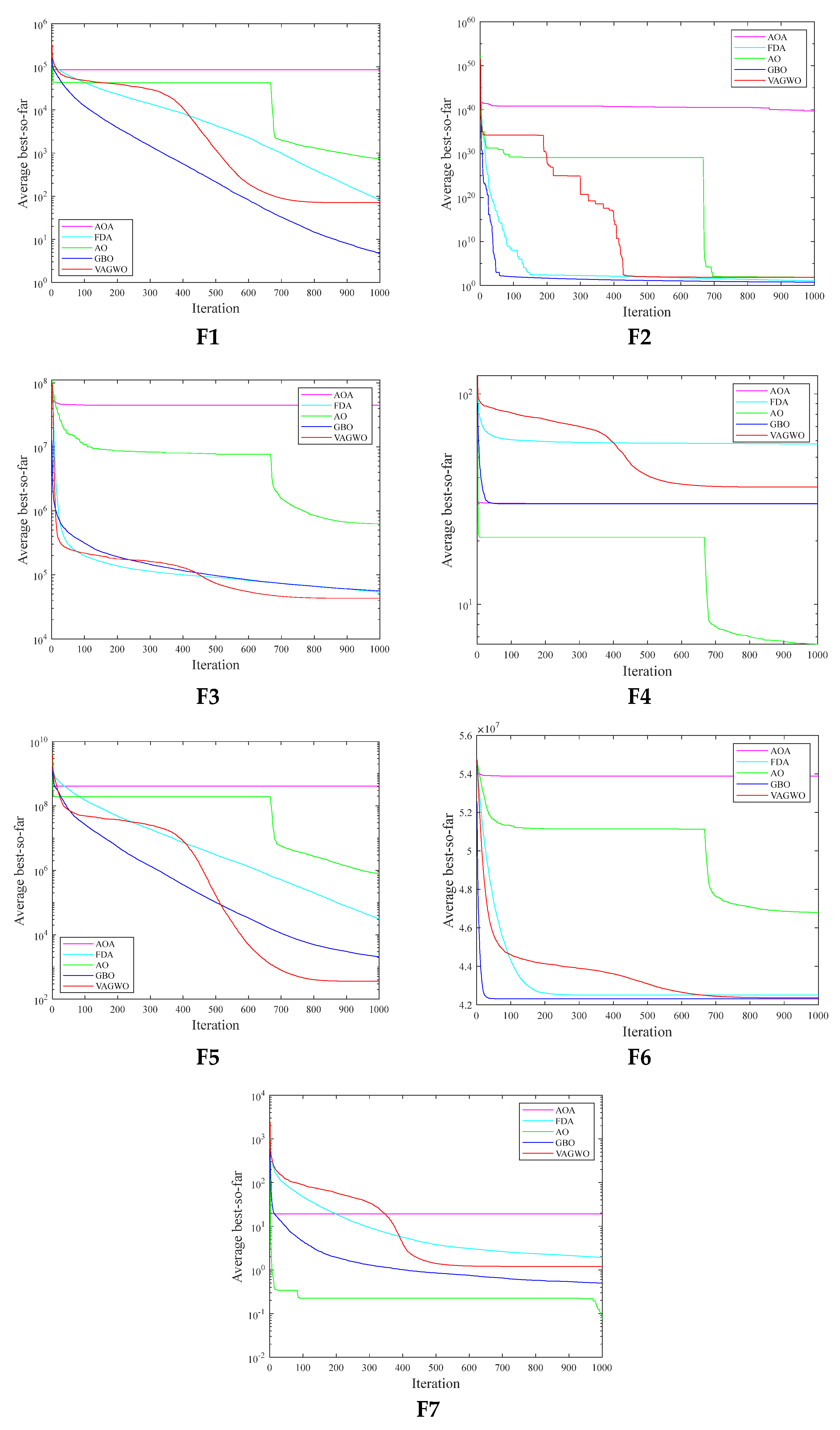
3.2.1. Results of VAGWO on the Uni-Modal Benchmark Functions

As the results illustrated in Table 6 suggest, the VAGWO outperforms the other competing algorithms on 10 out of 28 (36%) of the performance criteria on the uni-modal functions. The closest rivals to the VAGWO based on this category of benchmarks are GBO and AO algorithms, outperforming the others on 10 out of 28 (36%) and 8 out of 28 (29%) of the criteria, respectively. As can be seen, the results suggest the superiority of the VAGWO as compared to the other competitive algorithms.

Although the exploitation capability of the original GWO algorithm is strong, adding the velocity term to the updating procedure of the search agents in the VAGWO can expedite their convergence to the optimal point, and thus the superiority of the VAGWO on these functions may be realizable. Among the other features of the VAGWO contributing to this algorithm to show better exploitation, incorporating an elitism mechanism along with some crucial modifications especially on the coefficients C which are multiplied by the leading wolves’ position to take uncertainty in their fitness can be mentioned.

The convergence curves depicted in Figure 5 show that the VAGWO can converge to the optimum on F2, F3, F5, and F6, with a rate better than or equal to the other competing algorithms. The most serious rival of the VAGWO is GBO, which is very similar to the proposal in behavior when conducting the optimization process on the uni-modal functions.

3.2.2. Results of VAGWO on the Multi-Modal Benchmark Functions

As the results displayed in Table 7 suggest, the VAGWO is highly superior to its competitors on F10-F12, while the superiority on the other functions in this category is dispersed among the other algorithms. On F13, the results of the VAGWO are very close to those of the FDA, AO, and GBO, while being far better than those of the AOA. Benefiting from a velocity-aided updating procedure as well as accelerating the exploration via increasing the coefficients A at the early stages of the optimization process are among the two major factors leading to the superiority of the VAGWO in solving this category of function when compared to its rivals.

The convergence curves are shown in Figure 6. As indicated in this figure, the VAGWO rapidly and greedily converges to the optimal point of F10–F13, while its closest rival, namely the GBO, seems to stagnate during the optimization of all functions after the lapse of several iterations.

3.2.3. Comparison on CEC2017 Benchmark Functions

The VAGWO is investigated to reveal if its superiorioty to the popular algorithms on the composition functions derived from the CEC2017 benchmark suite is continued when compared to the newly proposed algorithms and the winner of the CEC2017 competition under the same conditions. As can be seen in Table 8, the VAGWO is superior to its competitors on CF1, CF3, CF4, CF6, CF7, CF8, and CF9. Overall, the VAGWO is superior to the other algorithms on 23 out of 40 criteria (58%), while its closest rival is found to be the EBOwithCMAR, as the winner of the CEC2017 competition, which can outperform the other methods only on 20% of the whole criteria. This category of test problems can be a very good examiner of the overall eligibility of any optimization algorithm, as it contains the toughest problems to solve. Adding the velocity term, defining a new formulation for the coefficients C, accelerating the exploration and exploitation in the early and later iterations, respectively, and also incorporating an elitism mechanism are all among the strengths of the proposed VAGWO, helping this algorithm to even overcome the newly proposed meta-heuristics and the winner of the CEC2017 competition.

3.3. Statistical Analysis

To further analyze the results, a non-parametric test, named the Wilcoxon rank-sum test, is applied to delineate whether two sets of results are statistically different [42]. This test presents a parameter called the p-value to determine the significance level of a pair of results generated by a pair of algorithms. Usually, the superiority of the performance of a method is statistically significant when the p-value < 0.05.

The p-values are presented in

Table 9. p-values and signs of the Wilcoxon test for VAGWO against the popular algorithms on the standard functions.

	GA		GSA		GWO		SCA		MFO		PSO		VAGWO
F1	0.0286	+	0.0286	+	0.0286	+	0.0286	+	0.0286	+	0.0286	+	N/A	$~$
F2	0.1429	−	0.0286	+	0.0286	+	0.0286	+	0.0286	+	N/A	$~$	0.0286	+
F3	0.0286	+	0.0286	+	0.0286	+	0.0286	+	0.0286	+	0.0286	+	N/A	$~$
F4	0.0286	+	0.0286	+	N/A	$~$	0.0286	+	0.0286	+	0.0286	+	0.0286	+
F5	0.0286	+	0.0286	+	0.0286	+	0.0286	+	0.1429	+	0.0286	+	N/A	$~$
F6	0.0286	+	0.0286	+	0.0286	+	0.0286	+	0.0286	−	0.0286	+	N/A	$~$
F7	0.0286	+	0.0286	+	0.0286	+	0.0286	+	0.0286	+	0.0286	+	N/A	$~$
F8	0.0286	+	0.0571	−	0.0286	+	0.1429	−	0.0286	+	N/A	$~$	0.0286	+
F9	0.0571	−	N/A	$~$	0.1429	−	0.0286	+	0.1429	+	0.0286	+	0.0286	+
F10	0.0571	−	0.0571	−	0.0571	−	0.0571	−	0.0286	−	0.0286	+	N/A	$~$
F11	0.0286	+	0.0286	+	0.0286	+	0.0286	+	0.0286	+	0.0286	+	N/A	$~$
F12	0.0286	+	0.0286	+	0.0286	+	0.0286	+	0.1429	+	0.0286	+	N/A	$~$
F13	0.0286	+	0.0286	+	0.0286	+	0.0286	+	0.0286	−	0.0286	+	N/A	$~$

,

Table 10. p-values and signs of Wilcoxon test for VAGWO against the popular algorithms on the CEC2017 composition functions.

	GA		GSA		GWO		SCA		MFO		PSO		VAGWO
CF1	0.3143	−	0.3143	−	0.3143	−	0.4857	−	0.3143	−	0.3143	−	N/A	$~$
CF2	0.8857	−	0.3429	−	N/A	$~$	0.2286	−	0.8857	−	0.3714	−	0.9714	+
CF3	0.3143	−	0.0286	+	0.4857	−	0.2000	−	0.3143	−	0.3143	−	N/A	$~$
CF4	0.3143	−	0.1429	−	0.3143	−	0.4857	−	0.3143	−	0.3143	−	N/A	$~$
CF5	0.0286	+	0.0286	+	0.0286	+	0.0286	+	0.0286	+	0.0286	+	N/A	$~$
CF6	0.0571	−	0.0571	−	0.6571	−	0.0571	−	0.3143	−	1.0000	$~$	N/A	$~$
CF7	0.0286	+	0.0286	+	0.0286	+	0.0286	+	0.0286	+	0.0286	+	N/A	$~$
CF8	0.0286	+	0.0286	+	0.0286	+	0.0286	+	0.0286	+	0.0286	+	N/A	$~$
CF9	0.0286	+	0.0286	+	0.0286	+	0.0286	+	0.0286	+	N/A	$~$	0.0286	+
CF10	0.0286	+	0.0286	+	0.0286	+	0.0286	+	0.0286	+	N/A	$~$	0.0286	+

,

Table 11. p-values and signs of Wilcoxon test for VAGWO against the newly proposed algorithms on the standard functions.

	AOA		FDA		AO		GBO		VAGWO
F1	0.0286	+	0.0286	+	0.0286	+	N/A	$~$	0.6571	−
F2	0.0286	+	0.0286	+	0.0286	+	N/A	$~$	0.0286	+
F3	0.0286	+	0.3143	−	0.1429	−	0.3143	−	N/A	$~$
F4	0.0571	−	0.0286	+	N/A	$~$	0.1429	−	0.0286	+
F5	0.0286	+	0.0286	+	0.0286	+	0.0286	+	N/A	$~$
F6	0.0286	+	0.2571	−	0.0286	+	N/A	$~$	0.3714	−
F7	0.0286	+	0.0286	+	N/A	$~$	0.0286	+	0.0286	+
F8	0.1429	−	0.2000	−	0.0857	−	N/A	$~$	0.0286	+
F9	0.1429	−	0.0286	+	N/A	$~$	0.0571	−	0.0286	+
F10	0.1429	−	0.0571	−	0.0286	+	0.0286	+	N/A	$~$
F11	0.0286	+	0.0286	+	0.0286	+	0.0286	+	N/A	$~$
F12	0.0286	+	0.0286	+	0.0286	+	0.0286	+	N/A	$~$
F13	0.0286	+	1	$~$	0.4286	−	N/A	$~$	0.0286	+

and

Table 12. p-values and signs of Wilcoxon test for VAGWO against the newly proposed algorithms on the CEC2017 functions.

	AOA		FDA		AO		GBO		EBOwithCMAR		VAGWO
CF1	0.1429	−	0.3143	−	0.3143	−	0.3143	−	0.4857	−	N/A	$~$
CF2	0.1429	−	0.3143	−	0.0857	−	0.2000	−	N/A	$~$	0.0857	−
CF3	0.0286	+	0.3143	−	0.2000	−	0.4857	−	0.3143	−	N/A	$~$
CF4	0.0286	+	0.4857	−	0.3143	−	0.3143	−	0.3143	−	N/A	$~$
CF5	0.0286	+	0.3143	−	0.0286	+	0.6571	−	N/A	$~$	1	$~$
CF6	0.0571	−	0.1143	−	0.0286	+	0.3143	−	0.3143	−	N/A	$~$
CF7	0.0286	+	0.0286	+	0.0286	+	0.0286	+	0.0286	+	N/A	$~$
CF8	0.0286	+	0.0286	+	0.0286	+	0.0286	+	0.2571	−	N/A	$~$
CF9	0.0286	+	0.0286	+	0.0286	+	0.0286	+	0.0286	+	N/A	$~$
CF10	0.0286	+	0.1429	−	0.0286	+	N/A	$~$	0.0286	+	0.0286	+

. In these tables, the expression N/A stands for “Not Applicable”, indicating a certain algorithm that outperforms the others in the quality of the results it presents in each test problem and thus should be compared pairwise with each of the other algorithms. Moreover, the signs “+”, “−“, and “$~$”, mean that the N/A algorithm beats, loses to, or ties with the other algorithms at the test, respectively. The results are broken down into two categories: (1) the results on the 13 shifted standard test functions; and (2) the results on the CEC2017 50-dimensional composition benchmark functions. As can be seen, the VAGWO significantly outperforms the popular meta-heuristic algorithms on 47 out of 54 (87%) of the total cases of its outperformance when applied to the standard functions. The VAGWO also shows significant dominance in 19 out of 42 (45%) of cases over the popular meta-heuristics when implemented on the CEC2017 composition functions.

Furthermore, the VAGWO can significantly outperform the newly proposed meta-heuristics in 15 out of 20 (75%) of its dominance cases when applied to the standard benchmarks, closely followed by the GBO which significantly outperforms the other competitive algorithms in 12 out of 20 (60%) of its total outperformance cases. The proposal also shows significant outperformance in 17 out of 35 (49%) of its all dominance cases, when implemented on the CEC2017 functions, while the EBOwithCMAR and GBO show significant dominance only in 2 out of 10 (20%) and four out of five cases (80%) of their total cases of outperformance, respectively. As a result, not only can the proposed VAGWO outperform the two sets of popular and newly proposed meta-heuristic algorithms as well as the winner of the CEC2017 competition when optimizing the two sets of the test functions, but it can also present significantly better results compared to its rivals.

3.4. Complexity of Algorithm

The complexity of VAGWO and GWO methods is evaluated according to the standard approach proposed in [35]. The results can be observed in

Table 13. The computational complexity of VAGWO against GWO.

	${\mathit{T}}_0$	${\mathit{T}}_1$	${\hat{\mathit{T}}}_2$		$({\hat{\mathit{T}}}_2-{\mathit{T}}_1)/{\mathit{T}}_0$
Algorithm	-	-	GWO	VAGWO	GWO	VAGWO
D = 10	0.0230	1.0960	4.2059	5.0984	135.1543	173.9418
D = 30	0.0230	2.5317	11.8755	13.7169	406.0756	486.1017
D = 50	0.0230	4.3593	19.2003	23.2219	644.9804	819.7566

, where $T_0$ stands for the computing time(s) for a standard loop illustrated in Figure 7, $T_1$ denotes the CPU time(s) of F18 from CEC2017 using 200,000 function evaluations, and ${\hat{T}}_2$ represents the average of CPU time(s) of the methods when solving the same function (i.e., F18) five times. The lowest complexities are highlighted in Table 13.

As can be observed from Table 13, the complexity of the VAGWO method is 29%, 20%, and 27% greater than that of the GWO for 10-, 30-, and 50-dimensional problems, respectively. As inferred from Table 13, the complexity of the proposed VAGWO is just a little greater than that of the GWO as its base algorithm, and their difference in complexity can even be reduced by increasing the dimensions of the problem. It is worth mentioning that all algorithms were run in the MATLAB-R2018b environment installed on the Windows 10 operating system of an Intel Quad-core computer with 2.8 GHz CPU and 16 GB of memory.

3.5. Runtime Analysis

The runtime of VAGWO and GWO algorithms is evaluated to better understand if the proposed algorithm retains its efficiency despite its increased complexity as compared to the original GWO.

Table 14. The independent runtime of VAGWO against GWO on the standard functions (seconds).

	GWO	VAGWO
F1	5.30	5.55
F2	5.12	5.65
F3	5.42	6.30
F4	5.36	5.62
F5	4.96	5.50
F6	5.35	6.05
F7	5.53	5.83
F8	5.30	6.11
F9	5.13	6.16
F10	5.21	5.96
F11	5.19	6.10
F12	5.65	5.80
F13	5.75	6.59
Average	5.33	5.94

and

Table 15. The independent runtime of VAGWO against GWO on the CEC2017 composition functions (seconds).

	GWO	VAGWO
CF1	5.81	5.89
CF2	5.54	6.40
CF3	5.76	6.55
CF4	5.88	6.71
CF5	5.81	6.56
CF6	6.11	6.94
CF7	6.37	7.21
CF8	6.14	6.64
CF9	5.89	6.02
CF10	7.29	7.44
Average	6.06	6.64

show the results of the runtime of independent executions of each test problem, including the standard benchmark functions and the CEC2017 composition functions, respectively. These runtimes are the average of the runtimes of the algorithms when executed 30 times. As the results suggest, the average runtime of the GWO is calculated to be 5.33 s on the standard functions, while the average runtime of the VAGWO on the same functions is evaluated to be 5.94 s, indicating just an 11.45% increase in runtime when using the proposed VAGWO to solve these benchmarks. Moreover, the average runtime of the GWO is obtained as 6.06 s on the CEC2017 composition functions, while the VAGWO has an average runtime of 6.64 s on these functions, showing just a 9.51% increase in runtime compared to that of the GWO. As can be seen, the runtime and consequently the complexity of the VAGWO is just slightly greater than the original GWO, revealing that the proposed algorithm can reach highly better results than the GWO while preserving its efficiency. Meanwhile, the difference in the runtime of the two algorithms is lessened when implemented on the CEC2017 functions. As the CEC2017 functions are much more complex functions to evaluate than the standard functions, it can be inferred that the main reason causing the complexity of the proposed VAGWO to be lessened on the CEC2017 is that the objective function evaluations of this test set are assigned a high weight in the complexity of any algorithm employed to optimize these functions. As a result, the complexity of the main body of the VAGWO algorithm can find less weight in the total complexity of a single run of the optimization process of the CEC2017 functions than that when applied to the standard functions. This point is very promising and further encourages the use of the VAGWO, especially when dealing with a complex objective function.

3.6. Comparison on Real-World Engineering Design Problems

In this section, the performance of the VAGWO is examined by solving three constrained real-world engineering design problems. To validate the VAGWO in solving such problems, the resulting performance of VAGWO is tested against seven state-of-the-art and widely used optimization algorithms, including Particle Swarm Optimization (PSO) [38], Gravitational Search Algorithm (GSA) [37], Cuckoo Search (CS) [3], Grey Wolf Optimizer (GWO) [4], Whale Optimization Algorithm (WOA) [7], Elephant Herding Optimizer (EHO) [43], and Simulated Annealing (SA) algorithm [44]. All the results of these algorithms taken to be compared with those achieved by the proposed VAGWO algorithm are presented in [45]. For handling the constraints in these problems, the scalable penalty functions are utilized in VAGWO and once the solutions become infeasible, numerous penalty functions are added to the minimization objective to enhance the cost of the optimization and penalize these solutions.

In addition, 50 search agents, as well as 1000 iterations, are used in VAGWO, and each problem is run 30 times, and the best results, including the best objective values and the best design variables are reported against those resulting from the other algorithms examined.

3.6.1. Welded Beam Design Problem

In this problem, a welded beam is designed to minimize its construction cost [46]. The main objective function is subject to some constraints. The problem includes four design variables consisting of $h\left(x_1\right)$, $l\left(x_2\right)$, $t\left(x_3\right)$, and $b\left(x_4\right)$, as shown in Figure 8. The formulation of this problem is as follows:

$$\mathit{Minimize}f\left(x\right)=1.10471x_1^2{x}_2+0.04811x_3{x}_4(14+x_2)$$

(29)

Subject to:

$$g_1\left(x\right)=\tau \left(x\right)-{\tau }_{\mathit{max}}\le 0$$

(30)

$$g_2\left(x\right)=\sigma \left(x\right)-{\sigma }_{\mathit{max}}\le 0$$

(31)

$$g_3\left(x\right)=x_1-x_4\le 0$$

(32)

$$g_4\left(x\right)=0.10471x_1^2+0.04811x_3{x}_4(14+x_2)-5\le 0$$

(33)

$$g_5\left(x\right)=0.125-x_1\le 0$$

(34)

$$g_6\left(x\right)=\delta \left(x\right)-{\delta }_{\mathit{max}}\le 0$$

(35)

$$g_7\left(x\right)=P-P_c\left(x\right)\le 0$$

(36)

$$0.1\le x_i\le 2,i=1,4$$

(37)

$$0.1\le x_i\le 10,i=2,3$$

(38)

where

$$\tau \left(x\right)=\sqrt{{{(\tau }^{\prime })}^2+{2\tau }^{\prime }{\tau }^{″}\frac{x_2}{2R}+{\left({\tau }^{″}\right)}^2}, {\tau }^{\prime }=\frac{P}{\sqrt{2}{x}_1{x}_2}, {\tau }^{″}=\frac{\mathit{MR}}{J}$$

(39)

$$M=P\left(L+\frac{x_2}{2}\right),R=\sqrt{\frac{x_2^2}{4}+{\left(\frac{x_1{+x}_3}{2}\right)}^2},J=2\left\{\sqrt{2}{x}_1{x}_2\left[\frac{x_2^2}{12}+{\left(\frac{x_1{+x}_3}{2}\right)}^2\right]\right\}$$

(40)

$$\sigma \left(x\right)=\frac{6\mathit{PL}}{x_4{x}_3^2},\delta \left(x\right)=\frac{{4\mathit{PL}}^3}{{\mathit{Ex}}_3^3{x}_4}{,P}_c\left(x\right)=\frac{4.013E\sqrt{\left(x_3^2{x}_4^6/36\right)}}{L^2}\left(1-\frac{x_3}{2L}\sqrt{\frac{E}{4G}}\right)$$

(41)

$${P=6000\mathit{lb},L=14\mathit{in},E=30\times 10}^6{\mathit{psi},G=12\times 10}^6\mathit{psi}$$

(42)

$${\tau }_{\mathit{max}}{=13,600\mathit{psi},\sigma }_{\mathit{max}}{=30,000\mathit{psi},\delta }_{\mathit{max}}=0.25\mathit{in}$$

(43)

Table 16. Minimization results of welded beam design.

Algorithm	h	L	t	b	f(x)
PSO	0.2157	3.4704	9.0356	0.2658	1.8578
GSA	0.2191	3.6661	10.0000	0.2508	2.2291
CS	0.2057	3.4705	9.0366	0.2057	1.7289
GWO	0.2054	3.4778	9.0388	0.2067	1.7265
WOA	0.1876	3.9298	8.9907	0.2308	1.9428
EHO	0.4834	2.4950	4.4538	0.8488	2.3234
SA	0.2055	3.4751	9.0417	0.2063	1.7306
VAGWO	0.2057	3.2531	9.0366	0.2057	1.6952

shows the results of solving the welded beam design problem obtained by the VAGWO and the other comparative algorithms. As can be seen, the VAGWO can reach $f\left(x\right)=1.6952$, which is the minimum and the best cost among the other algorithms. The design variables obtained by the VAGWO are shown in Table 16 and assumed as the best variables with respect to the objective function value the VAGWO can achieve during the optimization process.

3.6.2. Tension/Compression Spring Design Problem

The tension/compression spring design problem [48] aims to minimize the weight of a tension/compression spring, subject to constraints on minimum deflection, outside diameter restrictions, surge frequency, shear stress, and design variables. The design variables are $d\left(x_1\right)$, $D\left(x_2\right)$, and $P\left(x_3\right)$, as depicted in Figure 9. The formulation of this problem is as follows:

$$\mathit{Minimize}f\left(x\right)=(x_3+2)x_2{x}_1^2$$

(44)

Subject to:

$$g_1\left(x\right)=1-\frac{x_2^3{x}_3}{{71,785x}_1^4}\le 0$$

(45)

$$g_2\left(x\right)=\frac{{4x}_2^2-x_1{x}_2}{12,566\left(x_2{x}_1^3-x_1^4\right)}+\frac{1}{{5108x}_1^2}\le 0$$

(46)

$$g_3\left(x\right)=1-\frac{140.45x_1}{x_2^2{x}_3}\le 0$$

(47)

$$g_4\left(x\right)=\frac{x_1+x_2}{1.5}-1\le 0$$

(48)

$$0.05\le x_1\le 2.00$$

(49)

$$0.25\le x_2\le 1.30$$

(50)

$$2.00\le x_3\le 15.0$$

(51)

Table 17. Minimization results of tension/compression spring design.

Algorithm	d	D	N	f(x)
PSO	0.0514	0.3577	11.6187	0.0127
GSA	0.0500	0.3170	14.0802	0.0127
CS	0.0518	0.3586	11.1808	0.0127
GWO	0.0519	0.3627	10.9512	0.0127
WOA	0.0520	0.3637	10.8938	0.0127
EHO	0.0580	0.5278	5.5820	0.0135
SA	0.0500	0.2500	9.3876	0.0178
VAGWO	0.0518	0.3589	11.1648	0.0127

shows the final results the VAGWO and its competitors present after solving this problem. As shown in the table, the VAGWO achieves the minimum weight for the tension/compression spring, presenting $f\left(x\right)=1.2665\times {10}^{-2}$. The first five comparative algorithms yield the same objective function value, while the EHO and SA present the worst objective values among all the algorithms applied to this problem.

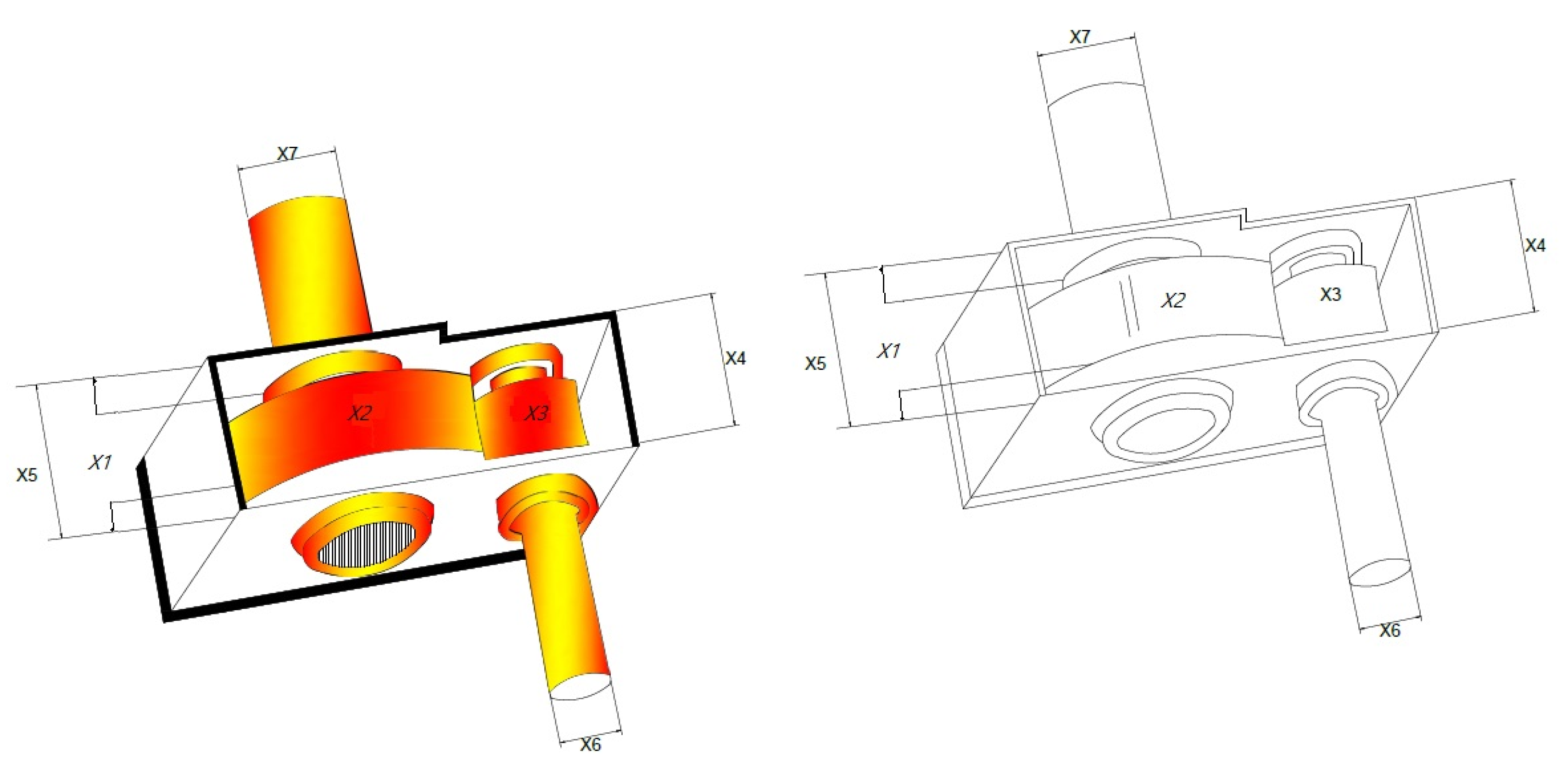
3.6.3. Speed Reducer Design Problem

This optimization problem is a constrained one, an similarly to the two previous problems it aims to minimize the weight of a speed reducer subject to constraints on the bending stress of the gear teeth, surface stress, transverse deflections of the shafts, and stresses in the shafts [49]. The scheme of the speed reducer is shown in Figure 10. The formulation of this problem is as follows:

$$\mathit{Minimize}f\left(x\right)=0.7854x_1{x}_2^2\left(\begin{array}{c}3.3333x_3^2+14.9334x_3-43.0934-1.508x_1\left(x_6^2{+x}_7^2\right)+\\ 7.4777\left(x_6^3+x_7^3\right)+0.7854{(x}_4{x}_6^2+x_5{x}_7^2)\end{array}\right)$$

(52)

Subject to:

$$g_1\left(x\right)=\frac{27}{x_1{x}_2^2{x}_3}-1\le 0$$

(53)

$$g_2\left(x\right)=\frac{397.5}{{71785x}_1^4}-1\le 0$$

(54)

$$g_3\left(x\right)=\frac{1.93x_4^3}{x_2{x}_6^4{x}_3}-1\le 0$$

(55)

$$g_4\left(x\right)=\frac{1.93x_5^3}{x_2{x}_7^4{x}_3}-1\le 0$$

(56)

$$g_5\left(x\right)=\frac{{\left[{\left(745\left(\frac{x_4}{x_2{x}_3}\right)\right)}^2+16.9\times {10}^6\right]}^{1/2}}{{110x}_6^3}-1\le 0$$

(57)

$$g_6\left(x\right)=\frac{{\left[{\left(745\left(\frac{x_5}{x_2{x}_3}\right)\right)}^2+157.5\times {10}^6\right]}^{1/2}}{{85x}_7^3}-1\le 0$$

(58)

$$g_7\left(x\right)=\frac{x_2{x}_3}{40}-1\le 0$$

(59)

$$g_8\left(x\right)=\frac{{5x}_2}{x_1}-1\le 0$$

(60)

$$g_9\left(x\right)=\frac{x_1}{{12x}_2}-1\le 0$$

(61)

$$g_{10}\left(x\right)=\frac{1.5x_6+1.9}{x_4}-1\le 0$$

(62)

$$g_{11}\left(x\right)=\frac{1.1x_7+1.9}{x_5}-1\le 0$$

(63)

$$2.6\le x_1\le 3.6$$

(64)

$$0.7\le x_2\le 0.8$$

(65)

$$17\le x_3\le 28$$

(66)

$$7.3\le x_4\le 8.3$$

(67)

$$7.3\le x_5\le 8.3$$

(68)

$$2.9\le x_6\le 3.9$$

(69)

$$5.0\le x_7\le 5.6$$

(70)

Table 18. Minimization results of speed reducer design.

Algorithm	x1	x2	x3	x4	x5	x6	x7	f(x)
PSO	3.5000	0.7000	17.0000	7.7400	7.8500	3.3600	5.3890	2998.1200
GSA	3.1530	0.7000	17.0000	7.3000	8.3000	3.2000	5.0000	3040.1000
CS	3.4970	0.7000	17.0000	7.3000	7.8000	3.3500	5.2800	2997.5000
GWO	3.5000	0.7000	17.0000	7.3000	7.8000	2.9000	2.9000	2998.8300
WOA	3.4210	0.7000	17.0000	7.3000	7.8000	2.9000	5.0000	2998.4000
EHO	2.9000	0.7000	17.0000	7.3000	7.8000	3.1000	5.2000	3019.0100
SA	2.7140	0.7050	17.9100	7.8500	7.8580	3.8800	5.2850	3000.4400
VAGWO	3.5615	0.7015	17.5633	7.9441	8.0719	3.5690	5.3402	3234.3413

shows the results obtained by the VAGWO and the other algorithms when solving this problem. As can be seen, the results of the different algorithms are very close to each other; however, the CS can achieve $f\left(x\right)=2.9975\times {10}^3$, as the best objective function value among all the other algorithms. The VAGWO reaches the most competitive result on this problem, as compared to the other examined algorithms. As a result, the VAGWO outperforms the other seven algorithms on two out of three examined real-world engineering design problems, demonstrating its efficacy in solving the constrained practical optimization problems along with a variety of high-dimensional and complex benchmark problems as well.

4. Conclusions

In this paper, a novel variant of the Grey Wolf Optimization (GWO) algorithm, named Velocity-Aided Grey Wolf Optimizer (VAGWO), was proposed. In this algorithm, a velocity term is added to the position-updating procedure of the original GWO algorithm. It was proven that the velocity can significantly improve the GWO algorithm when attempting to explore the search space, as the velocity can keep to push the search agents to continue their global search to prevent a considerable number of good positions being missed during the optimization process. In VAGWO, both the exploration and exploitation capabilities of the GWO are also strengthened via modification of the two control parameters of this algorithm. Furthermore, a safe and reliable balance between exploration and exploitation is maintained via emphasizing the position of the leading search agents in the last iterations and de-emphasizing them in the earlier iterations. Furthermore, an elitism mechanism is incorporated into the VAGWO to facilitate reaching the optimal solution via intensifying the exploitation. The proposed VAGWO was implemented on 13 shifted high-dimensional standard benchmark functions as well as a set of composition functions derived from the CEC2017 standard test functions and three real-world problems. The eligibility of the proposed method was then verified when compared with a set of popular and newly proposed meta-heuristic algorithms implemented on these test problems. A Wilcoxon test was also performed to highlight the significance of the superiority of the VAGWO when outperforming its competitors. The computational complexity of the VAGWO was also evaluated and demonstrated to be slightly greater than that of the original GWO algorithm. As a result, the proposal is a computationally efficient algorithm, while being capable of tackling the wide range of difficulties the different optimization problems experience. In future work, we will aim to extend the application of the VAGWO to other challenging theoretical and practical test problems to better identify its likely weaknesses and/or shortcomings and remove them to further ameliorate its functionality.

References

1. Engelbrecht, A.P. Computational Intelligence: An Introduction; Wiley: Hoboken, NJ, USA, 2007. [Google Scholar]
2. Yang, X.-S. Firefly Algorithms for Multimodal Optimization. In Stochastic Algorithms: Foundations and Applications; Watanabe, O., Zeugmann, T., Eds.; Springer: Berlin/Heidelberg, Germany, 2009; Volume 5792. [Google Scholar] [CrossRef] [Green Version]
3. Yang, X.-S.; Deb, S. Cuckoo Search via Lvy flights. In Proceedings of the 2009 World Congress Nature & Biologically Inspired Computing (NaBIC), Coimbatore, India, 9–11 December 2009; pp. 210–214. [Google Scholar] [CrossRef]
4. Mirjalili, S.; Mirjalili, S.M.; Lewis, A. Grey wolf optimizer. Adv. Eng. Softw. 2014, 6, 46–61. [Google Scholar] [CrossRef] [Green Version]
5. Mirjalili, S. Moth-flame optimization algorithm: A novel nature-inspired heuristic paradigm. Knowl. Based Syst. 2015, 89, 228–249. [Google Scholar] [CrossRef]
6. Ahmadianfar, I.; Bozorg-Haddad, O.; Chu, X. Gradient-based optimizer: A new metaheuristic optimization algorithm. Inf. Sci. 2020, 540, 131–159. [Google Scholar] [CrossRef]
7. Mirjalili, S.; Lewis, A. The whale optimization algorithm. Adv. Eng. Softw. 2016, 95, 51–67. [Google Scholar] [CrossRef]
8. Abualigah, L.; Mirjalili, S.; Elaziz, M.A.; Gandomi, A.H. The Arithmetic Optimization Algorithm. Comput. Methods Appl. Mech. Eng. 2021, 376, 113609. [Google Scholar] [CrossRef]
9. Abualigah, L.; Yousri, D.; Elaziz, M.A.; Ewees, A.A.; Al-qaness, M.A.A.; Gandomi, A.H. Aquila Optimizer: A novel meta-heuristic optimization algorithm. Comput. Ind. Eng. 2021, 157, 107250. [Google Scholar] [CrossRef]
10. Faris, H.; Aljarah, I.; Al-Betar, M.A.; Mirjalili, S. Grey wolf optimizer: A review of recent variants and applications. Neural Comput. Appl. 2018, 30, 413–435. [Google Scholar] [CrossRef]
11. Long, W.; Wu, T.; Cai, S.; Liang, X.; Jiao, J.; Xu, M. A Novel Grey Wolf Optimizer Algorithm with Refraction Learning. IEEE Access 2019, 7, 57805–57819. [Google Scholar] [CrossRef]
12. Long, W.; Jiao, J.; Liang, X.; Tang, M. Inspired grey wolf optimizer for solving large-scale function optimization problems. Appl. Math. Model. 2018, 60, 112–126. [Google Scholar] [CrossRef]
13. Mittal, N.; Singh, U.; Sohi, B.S. Modified Grey Wolf optimizer for global engineering optimization. Appl. Comput. Intell. Soft Comput. 2016, 2016, 7950348. [Google Scholar] [CrossRef] [Green Version]
14. Rodríguez, L.; Castillo, O.; Soria, J. Grey wolf optimizer with dynamic adaptation of parameters using fuzzy logic. In Proceedings of the 2016 IEEE Congress on Evolutionary Computation (CEC), Vancouver, BC, Canada, 24–29 July 2016; pp. 3116–3123. [Google Scholar]
15. Tawhid, M.A.; Ali, A.F. A hybrid grey wolf optimizer and genetic algorithm for minimizing potential energy function. Memetic Comput. 2017, 9, 347–359. [Google Scholar] [CrossRef]
16. Kamboj, V.K. A novel hybrid PSO-GWO approach for unit commitment problem. Neural Comput. Appl. 2016, 27, 1643–1655. [Google Scholar] [CrossRef]
17. Ibrahim, R.A.; Elaziz, M.A.; Lu, S. Chaotic opposition-based grey wolf optimization algorithm based on differential evolution and disruption operator for global optimization. Expert Syst. Appl. 2018, 108, 1–27. [Google Scholar] [CrossRef]
18. Niu, M.; Hu, Y.; Sun, S.; Liu, Y. A novel hybrid decomposition ensemble model based on VMD and HGWO for container throughput forecasting. Appl. Math. Model. 2018, 57, 163–178. [Google Scholar] [CrossRef]
19. Zhu, A.; Xu, C.; Li, Z.; Wu, J.; Liu, Z. Hybridizing grey Wolf optimization with differential evolution for global optimization and test scheduling for 3D stacked SoC. J. Syst. Eng. Electron. 2015, 26, 317–328. [Google Scholar] [CrossRef]
20. Luo, J.; Liu, Z. Novel grey wolf optimization based on modified differential evolution for numerical function optimization. Appl. Intell. 2020, 50, 468–486. [Google Scholar] [CrossRef]
21. Zhang, X.; Kang, Q.; Cheng, J.; Wang, X. A novel hybrid algorithm based on biogeography-based optimization and grey wolf optimizer. Appl. Soft Comput. 2018, 67, 197–214. [Google Scholar] [CrossRef]
22. Zhang, S.; Zhou, Y. Grey wolf optimizer based on Powell local optimization method for clustering analysis. Discret. Dyn. Nat. Soc. 2015, 2015, 481360. [Google Scholar] [CrossRef] [Green Version]
23. Mahdad, B.; Srairi, K. Blackout risk prevention in a smart grid based flexible optimal strategy using Grey Wolf-pattern search algorithms. Energy Convers. Manag. 2015, 98, 411–429. [Google Scholar] [CrossRef]
24. Oliveira, J.; Oliveira, P.M.; Boaventura-Cunha, J.; Pinho, T. Chaos based grey wolf optimizer for higher order sliding mode position control of a robotic manipulator. Nonlinear Dyn. 2017, 90, 1353–1362. [Google Scholar] [CrossRef]
25. Long, W.; Jiao, J.; Liang, X.; Tang, M. An exploration-enhanced grey wolf optimizer to solve high-dimensional numerical optimization. Eng. Appl. Artif. Intell. 2018, 68, 63–80. [Google Scholar] [CrossRef]
26. Jaiswal, K.; Mittal, H.; Kukreja, S. Randomized grey wolf optimizer (RGWO) with randomly weighted coefficients. In Proceedings of the 2017 Tenth International Conference on Contemporary Computing (IC3), Noida, India, 10–12 August 2017; pp. 1–3. [Google Scholar]
27. Chao, L.; Liang, G.; Jin, Y. Grey wolf optimizer with cellular topological structure. Expert Syst. Appl. 2018, 107, 89–114. [Google Scholar]
28. Rodríguez, L.; Castillo, O.; Soria, J.; Melin, P.; Valdez, F.; Gonzalez, C.I.; Martinez, G.E.; Soto, J. A fuzzy hierarchical operator in the grey wolf optimizer algorithm. Appl. Soft Comput. 2017, 57, 315–328. [Google Scholar] [CrossRef]
29. Hu, P.; Chen, S.; Huang, H.; Zhang, G.; Liu, L. Improved alpha-guided Grey wolf optimizer. IEEE Access 2019, 7, 5421–5437. [Google Scholar] [CrossRef]
30. Heidari, A.A.; Pahlavani, P. An efficient modified grey wolf optimizer with Lévy flight for optimization tasks. Appl. Soft. Comput. 2017, 60, 115–134. [Google Scholar] [CrossRef]
31. Gupta, S.; Deep, K. A novel random walk grey wolf optimizer. Swarm Evol. Comput. 2019, 44, 101–112. [Google Scholar] [CrossRef]
32. Yao, X.; Liu, Y.; Lin, G. Evolutionary programming made faster. IEEE Trans. Evol. Comput. 1999, 3, 82–102. [Google Scholar]
33. Suganthan, P.N.; Hansen, N.; Liang, J.J.; Deb, K.; Chen, Y.-P.; Auge, A.; Tiwari, S. Problem Definitions and Evaluation Criteria for the CEC 2005 Special Session on Real-Parameter Optimization; KanGAL Report 2005005; Kanpur Genetic Algorithms Laboratory: Kanpur, India, 2005. [Google Scholar]
34. Mirjalili, S. SCA: A Sine Cosine Algorithm for solving optimization problems. Knowl. Based Syst. 2016, 96, 120–133. [Google Scholar] [CrossRef]
35. Awad, N.H.; Ali, M.Z.; Suganthan, P.N.; Liang, J.J.; Qu, B.Y. Problem Definitions and Evaluation Criteria for the CEC 2017 Special Session and Competition on Single Objective Real-Parameter Numerical Optimization; Tech Rep; Nanyang Technological University: Singapore, November 2016. [Google Scholar]
36. Biondi, G.; Franzoni, V. Discovering correlation indices for link prediction using differential evolution. Mathematics 2020, 8, 2097. [Google Scholar] [CrossRef]
37. Rashedi, E.; Nezamabadi-Pour, H.; Saryazdi, S. GSA: A gravitational search algorithm. Inf. Sci. 2009, 179, 2232–2248. [Google Scholar] [CrossRef]
38. Kennedy, J.; Eberhart, R. Particle swarm optimization. In Proceedings of the IEEE International Conference on Neural Networks, Perth, WA, Australia, 27 November–1 December 1995; Volume IV, pp. 1942–1948. [Google Scholar]
39. Holland, J.H. Genetic algorithms. Sci. Am. 1992, 267, 66–72. [Google Scholar] [CrossRef]
40. Karami, H.; Anaraki, M.V.; Farzin, S.; Mirjalili, S. Flow Direction Algorithm (FDA): A novel optimization approach for solving optimization problems. Comput. Ind. Eng. 2021, 156, 107224. [Google Scholar] [CrossRef]
41. Kumar, A.; Misra, R.K.; Singh, D. Improving the local search capability of Effective Butterfly Optimizer using Covariance Matrix Adapted Retreat Phase. In Proceedings of the 2017 IEEE Congress on Evolutionary Computation (CEC), Donostia, Spain, 5–8 June 2017. [Google Scholar]
42. García, S.; Molina, D.; Lozano, M.; Herrera, F. A Study on the Use of Non-Parametric Tests for Analyzing the Evolutionary Algorithms’ Behaviour: A Case Study on the CEC’2005 Special Session on Real Parameter Optimization. J. Heuristics 2008, 15, 617–644. [Google Scholar] [CrossRef]
43. Wang, G.-G.; Deb, S.; Coelho, L.D.S. Elephant Herding Optimization. In Proceedings of the 3rd International Symposium on Computational and Business Intelligence (ISCBI), Bali, Indonesia, 7–9 December 2015. [Google Scholar]
44. Kirkpatrick, S.; Gelatt, C.D.; Vecchi, M.P. Optimization by simulated annealing. Science 1983, 220, 671–680. [Google Scholar] [CrossRef] [PubMed]
45. Hashim, F.A.; Houssein, E.H.; Mabrouk, M.S.; Al-Atabani, W.; Mirjalili, S. Henry gas solubility optimization: A novel physics-based algorithm. Future Gener. Comput. Syst. 2019, 101, 646–667. [Google Scholar] [CrossRef]
46. Coello, C.A.C. Use of a self-adaptive penalty approach for engineering optimization problems. Comput. Ind. 2000, 41, 113–127. [Google Scholar] [CrossRef]
47. Abualigah, L.; Elaziz, M.A.; Sumari, P.; Geem, Z.W.; Gandomi, A.H. Reptile Search Algorithm (RSA): A nature-inspired meta-heuristic optimizer. Expert Syst. Appl. 2022, 191, 116158. [Google Scholar] [CrossRef]
48. Arora, J.S. Introduction to Optimum Design; McGraw-Hill: New York, NY, USA, 1989. [Google Scholar]
49. Mezura-Montes, E.; Coello, C.A.C. Useful Infeasible Solutions in Engineering Optimization with Evolutionary Algorithms. In MICAI 2005: Advances in Artificial Intelligence; Springer: Berlin/Heidelberg, Germany, 2005; Volume 3789, pp. 652–662. [Google Scholar] [CrossRef]
Figure 1. Movement of an exemplary omega wolf in the VAGWO during (a) exploration; and (b) exploitation.
Mathematics 10 00351 g001
Figure 2. Flowchart of VAGWO.
Mathematics 10 00351 g002
Figure 3. The convergence curves of the VAGWO and the popular algorithms for F1–F7.
Mathematics 10 00351 g003
Figure 4. The convergence curves of the VAGWO and the popular algorithms for F8–F13.
Mathematics 10 00351 g004
Figure 5. The convergence curves of the VAGWO and the newly proposed algorithms for F1–F7.
Mathematics 10 00351 g005
Figure 6. The convergence curves of the VAGWO and the newly proposed algorithms for F8–F13.
Mathematics 10 00351 g006
Figure 7. The process of computing time T0.
Mathematics 10 00351 g007
Figure 8. Welded beam design problem [47].
Mathematics 10 00351 g008
Figure 9. Tension/compression spring problem [47].
Mathematics 10 00351 g009
Figure 10. Speed reducer design problem [47].
Mathematics 10 00351 g010