An Exact Solution to the Modified Winding Function for Eccentric Permanent Magnet Synchronous Machines

Abstract

The Winding Function Approach has been used since 1965 to describe the inductance behavior of small air-gap electrical machines, and several works have contributed to its formulation in the presence of mechanical faults, such as eccentricity, leading to the Modified Winding Function Approach (MWFA). In order to use the MWFA, an integral over a full rotation period needs to be computed. Nevertheless, this typically requires the performance of numerical integration, and thus it is affected by integration error, requires relatively high computational effort and, at the same time, it does not easily allow for performance of the analysis of the inductance harmonics. In this work, an exact analytical solution to the MWFA equation is provided in a form that allows to highlight the harmonic content of the inductances. After a thorough mathematical derivation of the solution, a numerical investigation is proposed for verification purposes.

1. Introduction

Permanent Magnet Synchronous Motors (PMSMs) are prominent nowadays in a variety of fields, such as mobility, industry, and home appliances mostly replacing DC and induction motors [1,2]. The main benefits compared to other drives are their high efficiency, lightweight structure, high power density, lower required maintenance, as well as a high and steady torque output [3,4,5]. Nevertheless, these machines require the rotor position information for proper driving [6], thus requiring the usage of an encoder that increases space requirements and costs. For this reason, several techniques have been proposed in the literature to overcome this limitation [7,8,9,10] that are mainly based on the exploitation of machine anisotropies or induced Back-Electro Motive Force (BEMF). Depending on the expected performance of the machine, the structure of PMSMs can vary. These variations can be classified according to the position of the permanent magnets on the rotor structure. If magnets are mounted on the surface of a cylindrical rotor, the machine is referred to as surface-mounted PMSM (SPMSM); otherwise, if magnets are buried in the rotor structure, the machine is referred to as an Interior PMSM (IPMSM).

Despite the robustness of PMSMs, machine failures can occur that can lead to the end of production or even life-endangering situations, such as motor failures occurring in transport and aerospace applications [11]. These events cannot only determine undesired situations, but also generate labor effort and high costs, both being direct and indirect. For this reason, failure prevention and condition monitoring techniques are of key importance in a majority of applications.

A straightforward way to prevent failure is inspecting all PMSMs on a regular basis. This, however, is not always possible, and in rare cases, profitable. Moreover, failures can still occur in between inspections. Instead, condition monitoring techniques are used to detect faults in a machine during operation. A survey about these techniques for rotating electrical machines can be found in the Ref. [12]. They can be classified in mechanical, chemical and electrical methods, although a number of novel methods, like the ones presented in the Ref. [13], use multi-parameter monitoring combined with a data-driven approach. Electrical fault detection methods are especially interesting for PMSMs, as some of them are based on quantities that are already measured to control the machine. This avoids the need for additional sensors, which are necessary for mechanical and chemical condition monitoring methods. Depending on the method, the typical measured electrical quantities include power, stator currents and voltages.

Machine faults can be categorized into mechanical, electrical and magnetic ones [14]. Mechanical faults are caused by material corrosion or fatigue, poor lubrication and an unbalanced rotor. These factors lead to eccentricity and, in the worst-case scenario, to a failure of the bearing. Electrical faults, such as a short circuit in the stator windings, are caused by overloading the machine, high temperature, and high stress. Magnetic faults include partial or anisotropic magnetization and, even worse, complete demagnetization. Causes for this are high temperature, mechanical stress and aging processes. It is fairly common that one of these faults quickly prompts additional faults even of another category (fault avalanche).

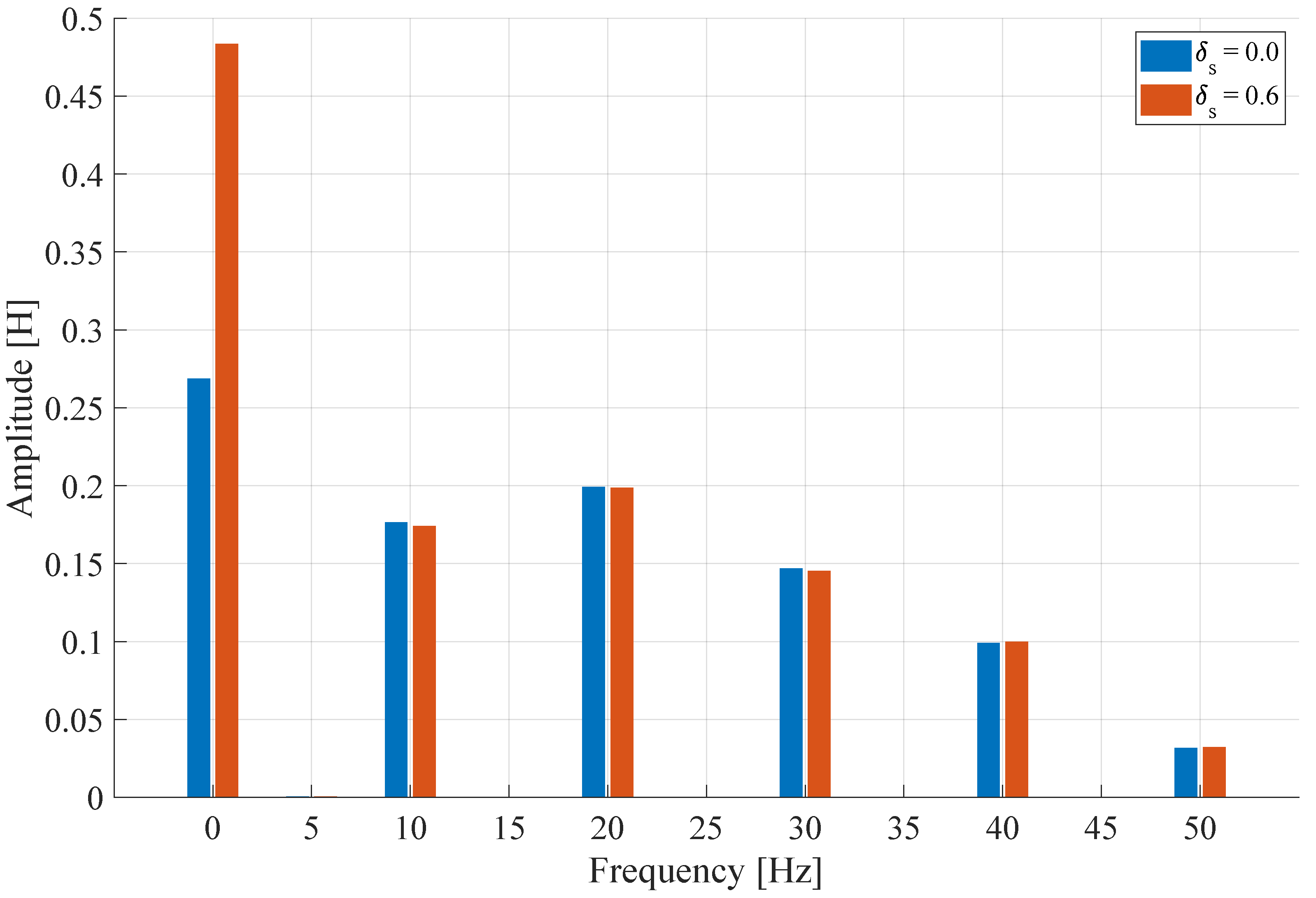
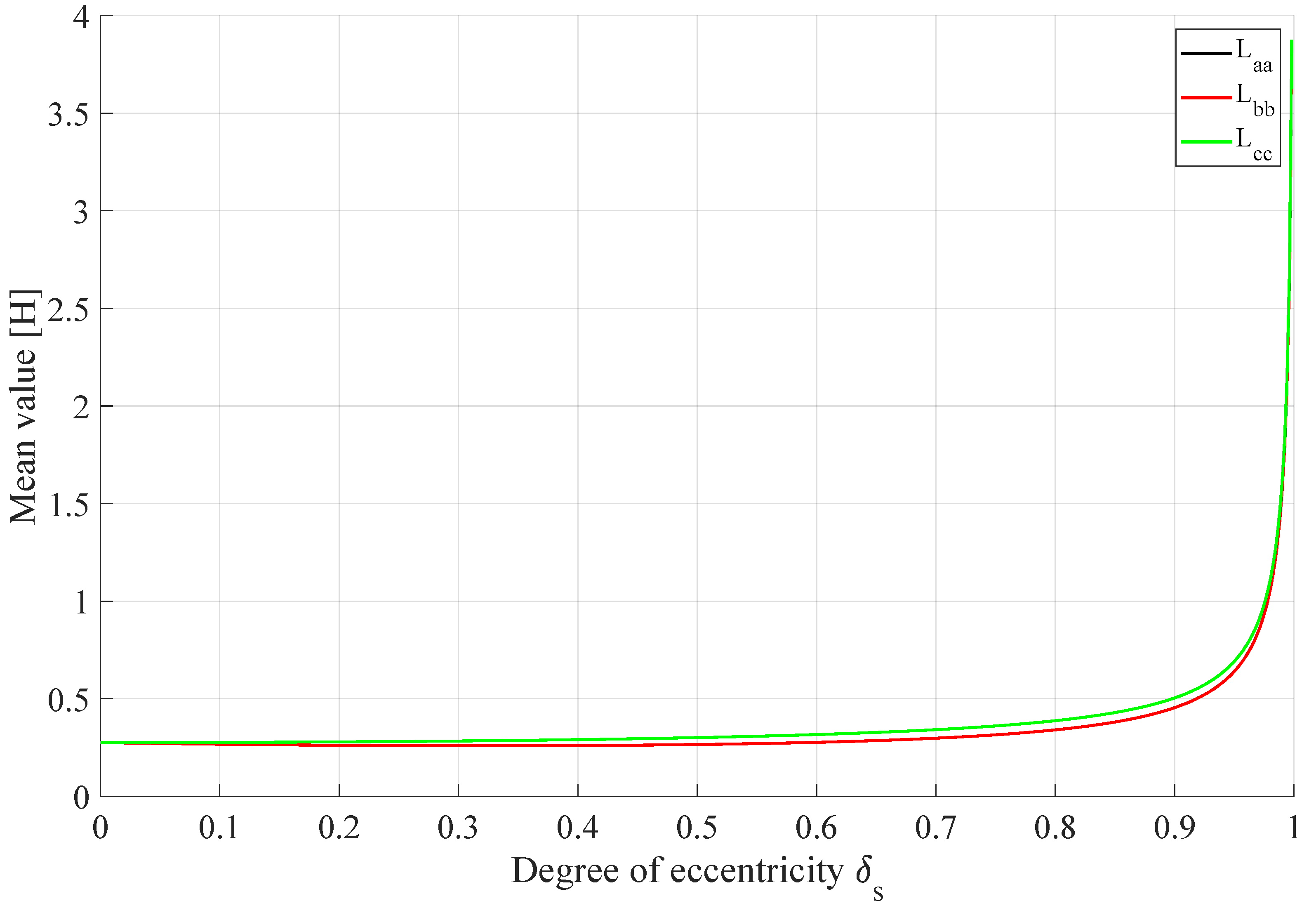
In particular, the works presented in the Refs. [15,16] trace the majority of failures occurring in induction machines back to mechanical issues. This data cannot simply be transferred to PMSMs, although it is safe to assume that PMSMs are also strongly affected by mechanical faults. Extensive reliability surveys for PMSMs are not yet available, as their mass application is fairly recent. As mentioned before, the main mechanical faults are eccentricity and bearing failures. With eccentricity being a big contributor to the failure of a bearing and a less obvious mechanical fault, it is a crucial parameter to monitor. This can be accomplished by means of mechanical sensors. Nevertheless, this approach would increase the size, cost and complexity of the overall system. Thus, another approach is the monitoring of the machine phase inductances. Indeed, the latter ones have a relatively strong dependency on eccentricity and, for this reason, any method based on their measurement and observation can be exploited for eccentricity detection.

The influence of eccentricity on the machine phase inductances can typically be observed by direct measurement on a test machine or by means of numerical methods and Finite Element Analysis. In any case, in order to fully analyze this dependency, it is very important to elaborate a mathematical model. This can be more easily numerically evaluated and provides, at the same time, a deeper insight into the dependency inductance, or eccentricity. One of the most frequently used starting points for numerical and analytical inductance models is the Modified Winding Function Approach (MWFA). Its general form is

$$L_{xy}\left(\theta \right)={\mu }_{0}rl{\int }_0^{2\pi }{N}_y(\phi ,\theta )n_x\left(\phi \right)g^{-1}(\phi ,\theta )d\phi ,$$

(1)

where x and y are arbitrary phases belonging to the set $\{A,B,C\}$ of the three-phase machine, ${\mu }_0$ is the permeability of the air-gap, r is the radius of the average air-gap, and l is the stack length of the machine. If $x=y$, Equation (1) describes a self-inductance, otherwise a mutual-inductance. The functions of Equation (1) are the modified winding function $N_x(\phi ,\theta )$, the turns function $n_x\left(\phi \right)$ and the inverse air-gap function $g^{-1}(\phi ,\theta )$, where $\theta$ is the rotor position and $\phi$ is an arbitrary angle in the stator reference frame.

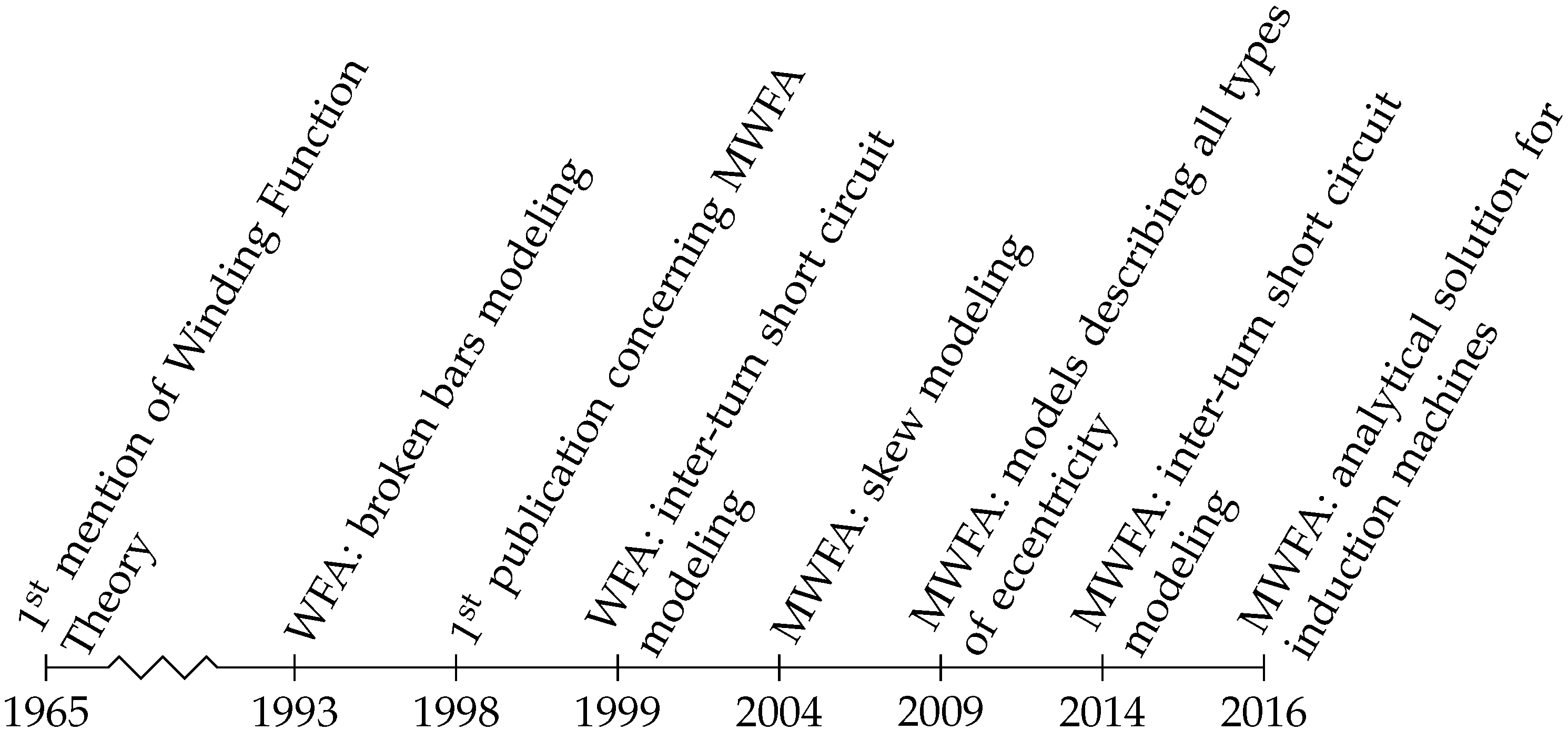
The Winding Function Approach (WFA) has been used extensively since at least 1965 [17] and has undergone major modifications and extensions over the last couple of decades, as illustrated in Figure 1. Using it, it is possible to model electrical machines based directly on the geometry and the physical layout of the winding. Although this approach is limited to a symmetrical air-gap, it is still applied to model healthy machines, as well as induction machines with broken bars and end rings [18] or inter-turn short circuits [19]. In order to extend this model to include machines with a non-symmetric air-gap, the MWFA was introduced in the Ref. [20]. Already in this first work, the MWFA was used to model dynamic eccentricity in a synchronous machine. Since then, it has been adopted to describe electrical machines in all kinds of conditions, such as skew [21], inter-turn short circuits [22] and, due to its modification, eccentricity [23]. In fact, models describing all types of eccentricity at once have been derived [24]. Most of these extensions to the MWFA, unfortunately, are based on inserting the specific functions into the general Equation (1) and performing a numerical integration. This is sufficient for most applications. However, an analytical solution would provide a meaningful insight into the dependency between eccentricity and machine phase inductances, making the MWFA more suitable for the synthesis of model-based fault detection techniques. There are several analytical inductance models which have been derived from the MWFA, but these are either restricted to a small number of harmonics or use a complex representation of the turns and air-gap functions [25]. Additionally, most models describe induction machines instead of PMSMs.

Simplifications while using the MWFA usually include a cylindrical stator shape and, therefore, the exclusion of slot openings, the permeability of the stator and rotor cores to be infinite compared to the air-gap material, and the use of linear materials. The last simplification is generally true in low-current or fully saturated conditions. Although there are a number of severe simplifications, reviews such as the Ref. [26] have found the MWFA to fit well to most electrical machines, although this work points out its limitations, including machines with large air-gaps.

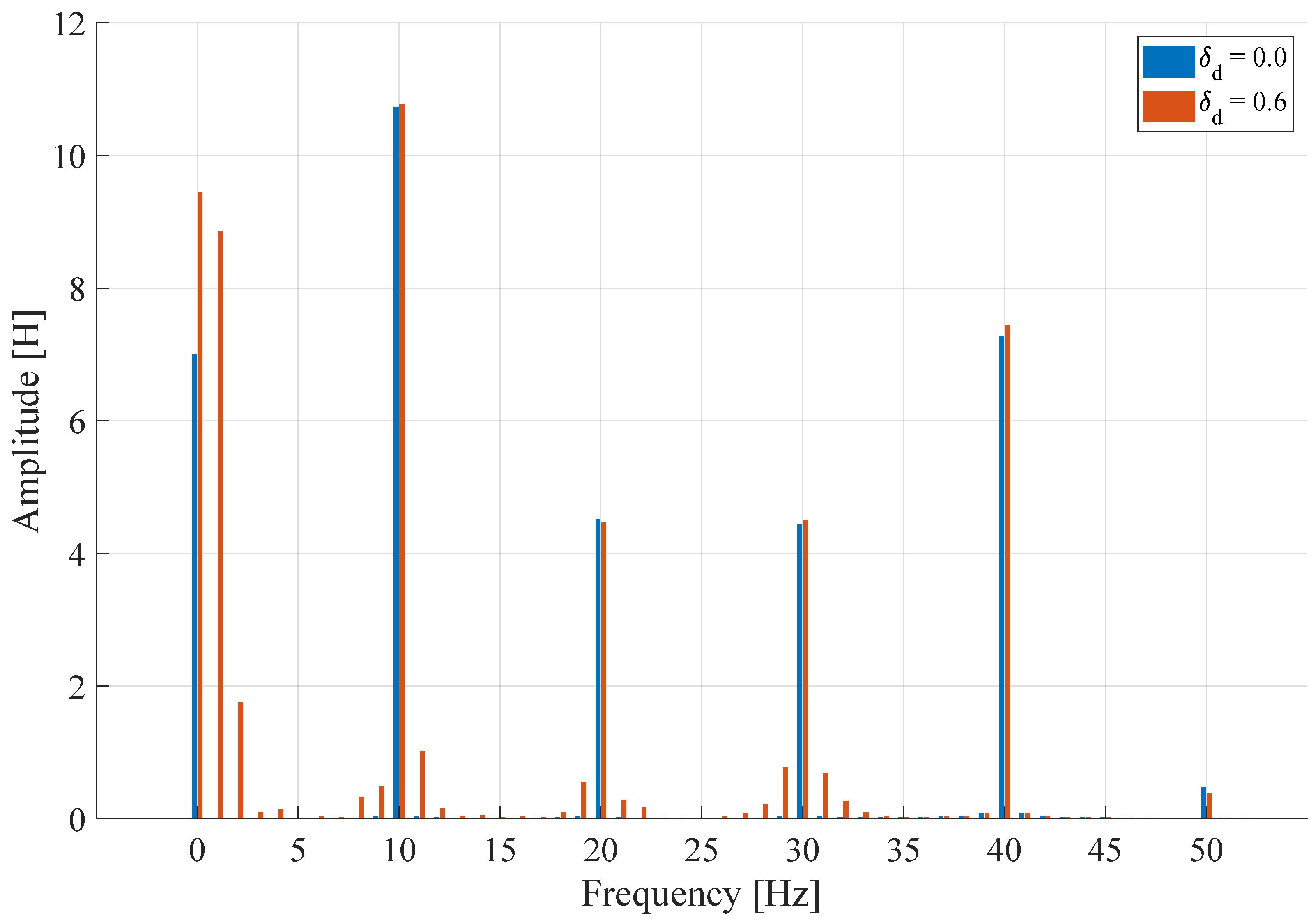
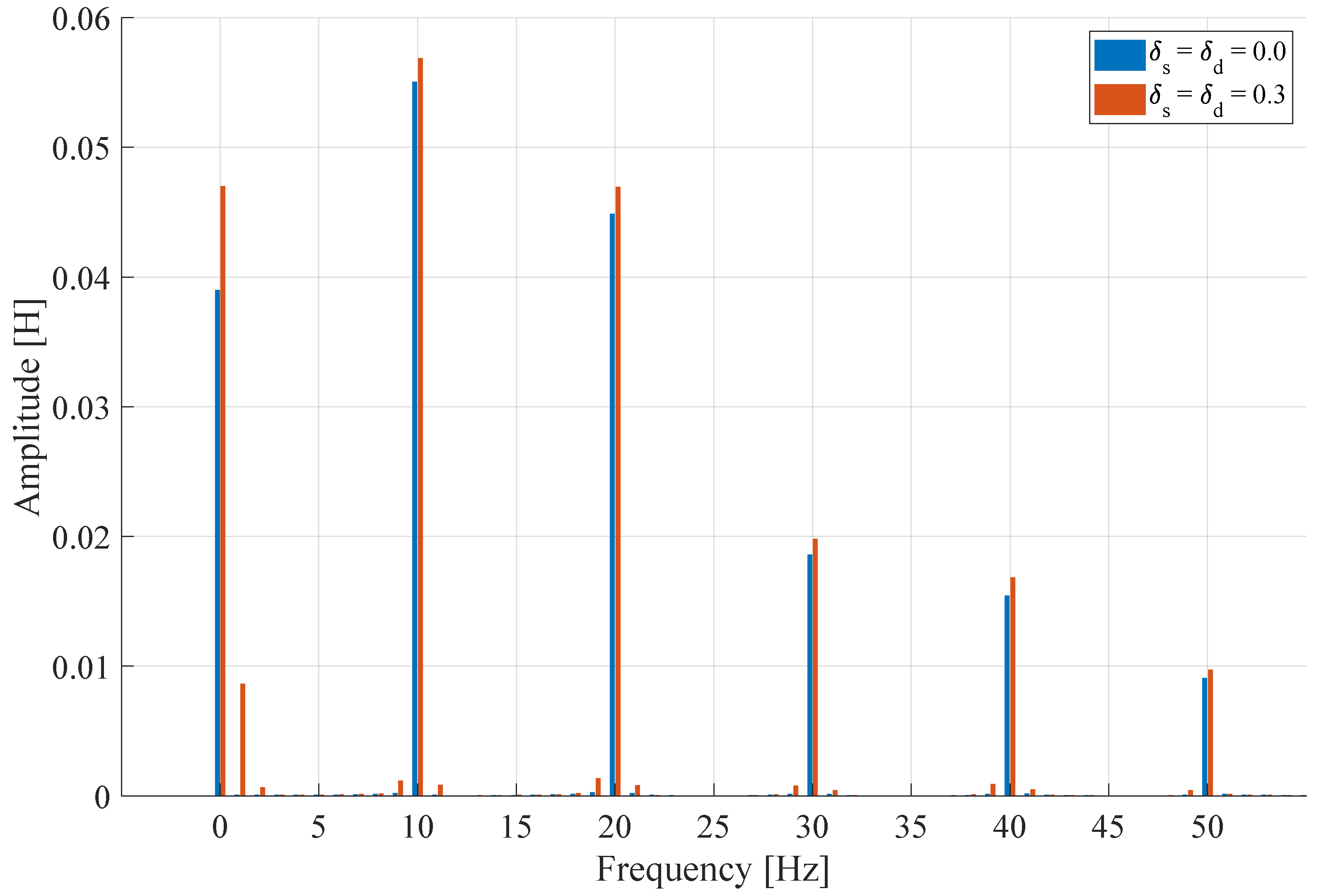
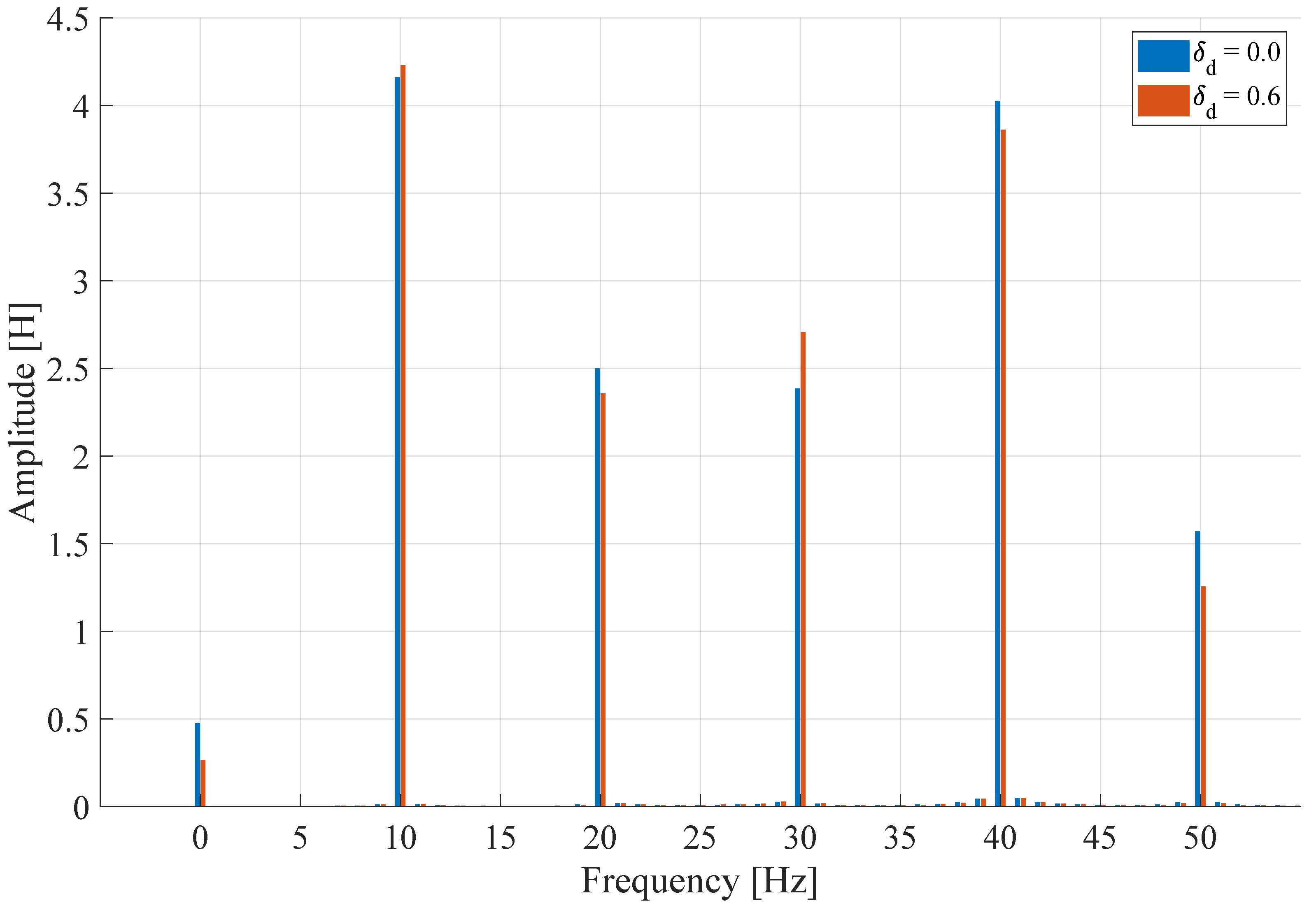
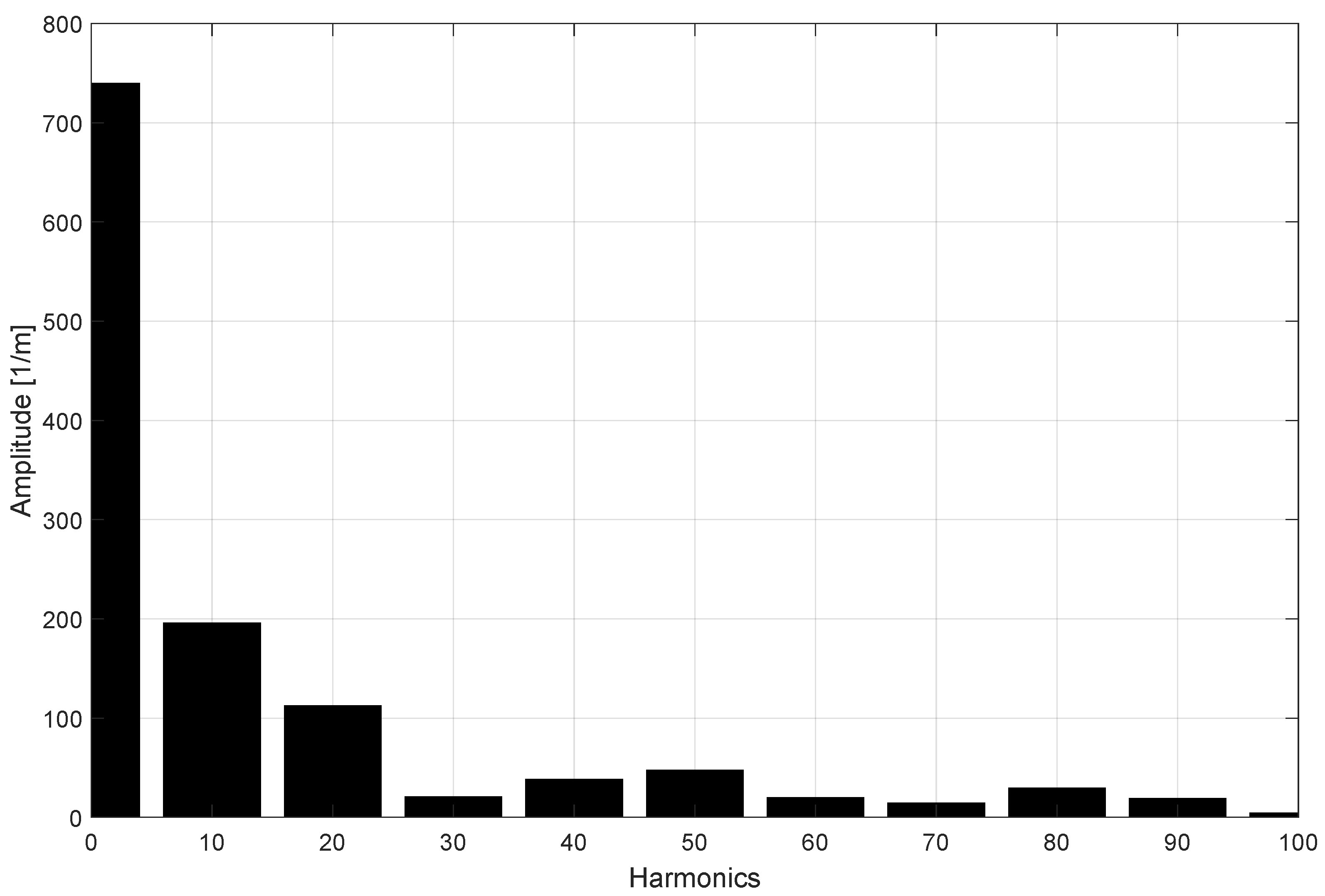
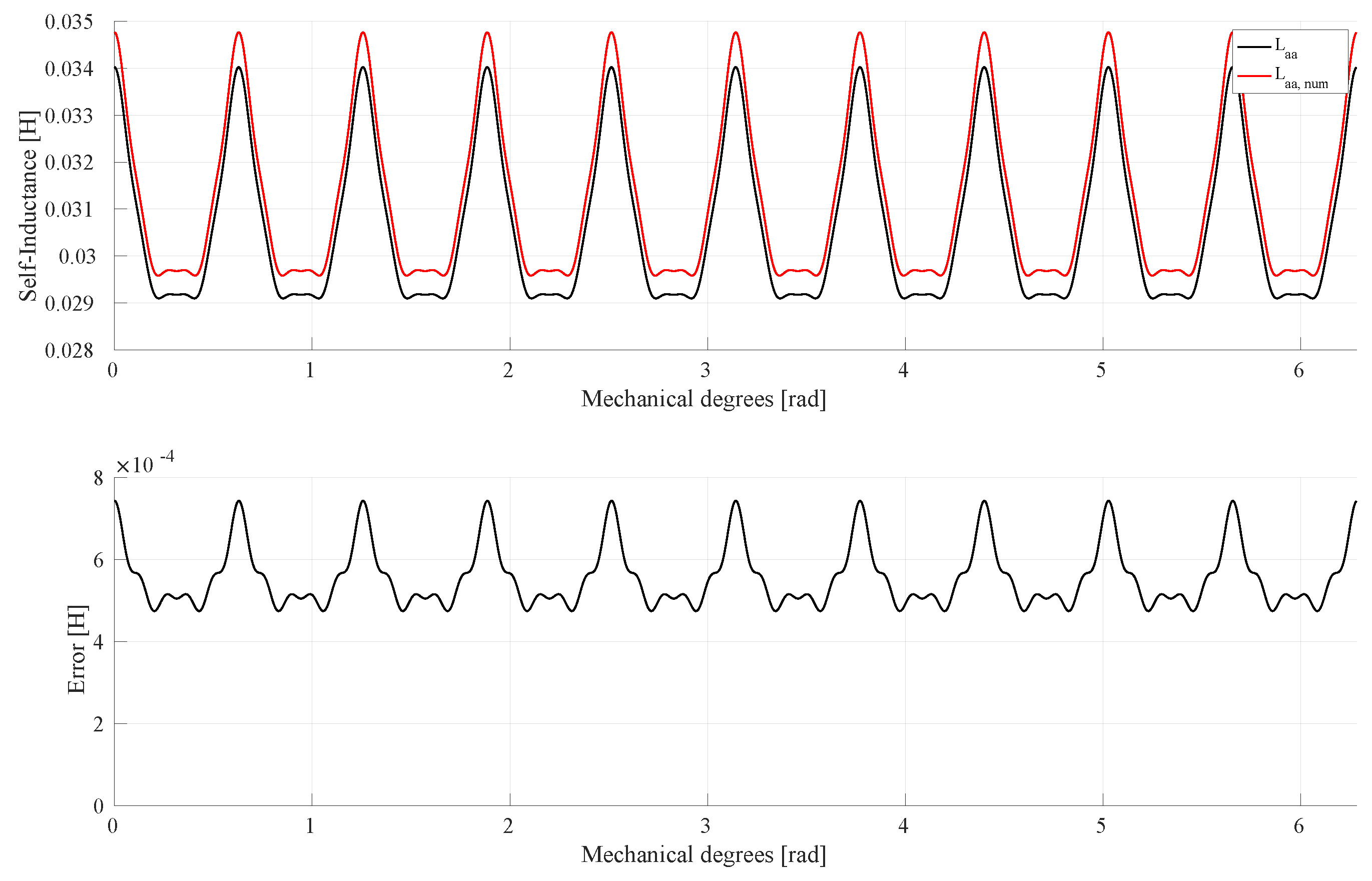
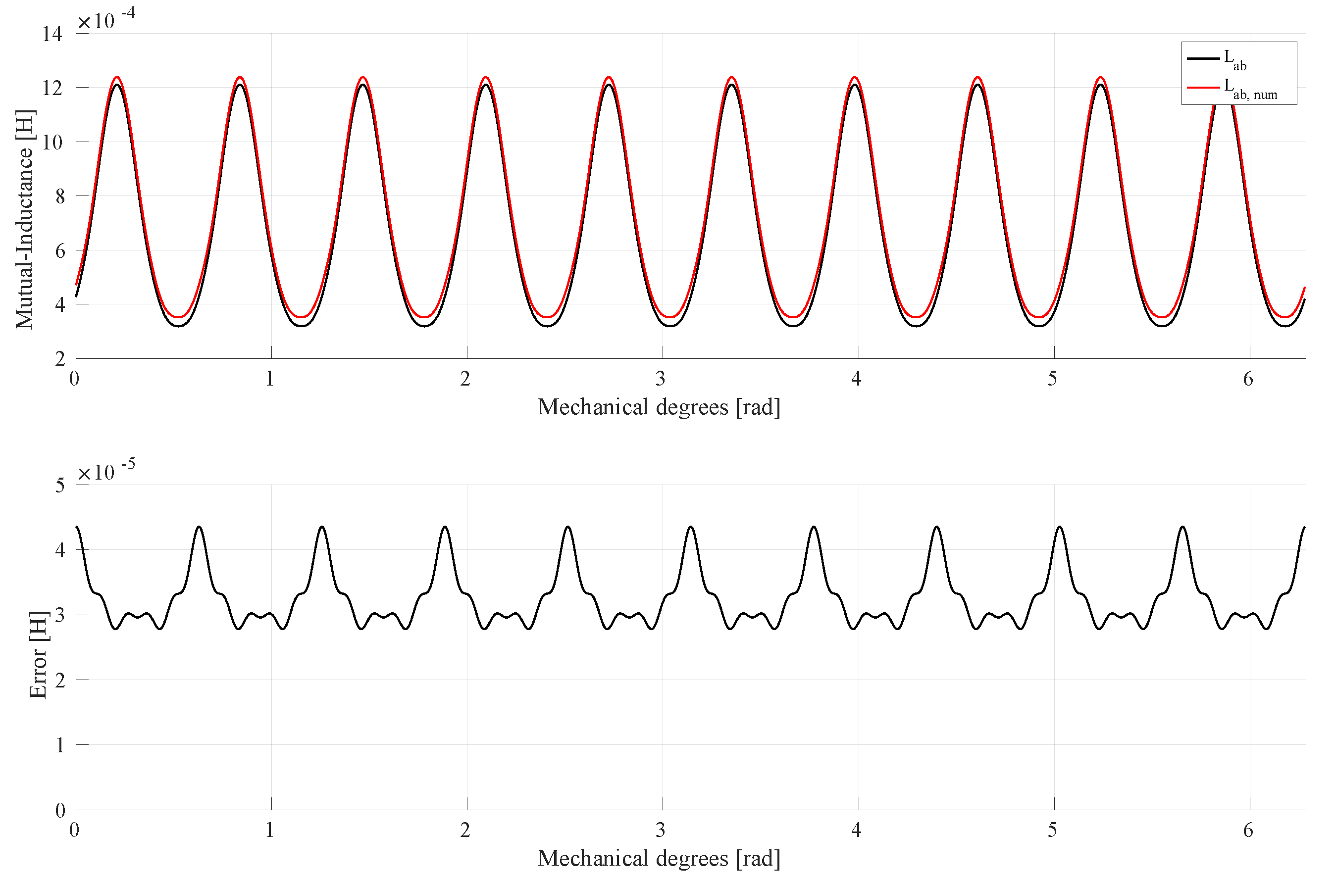
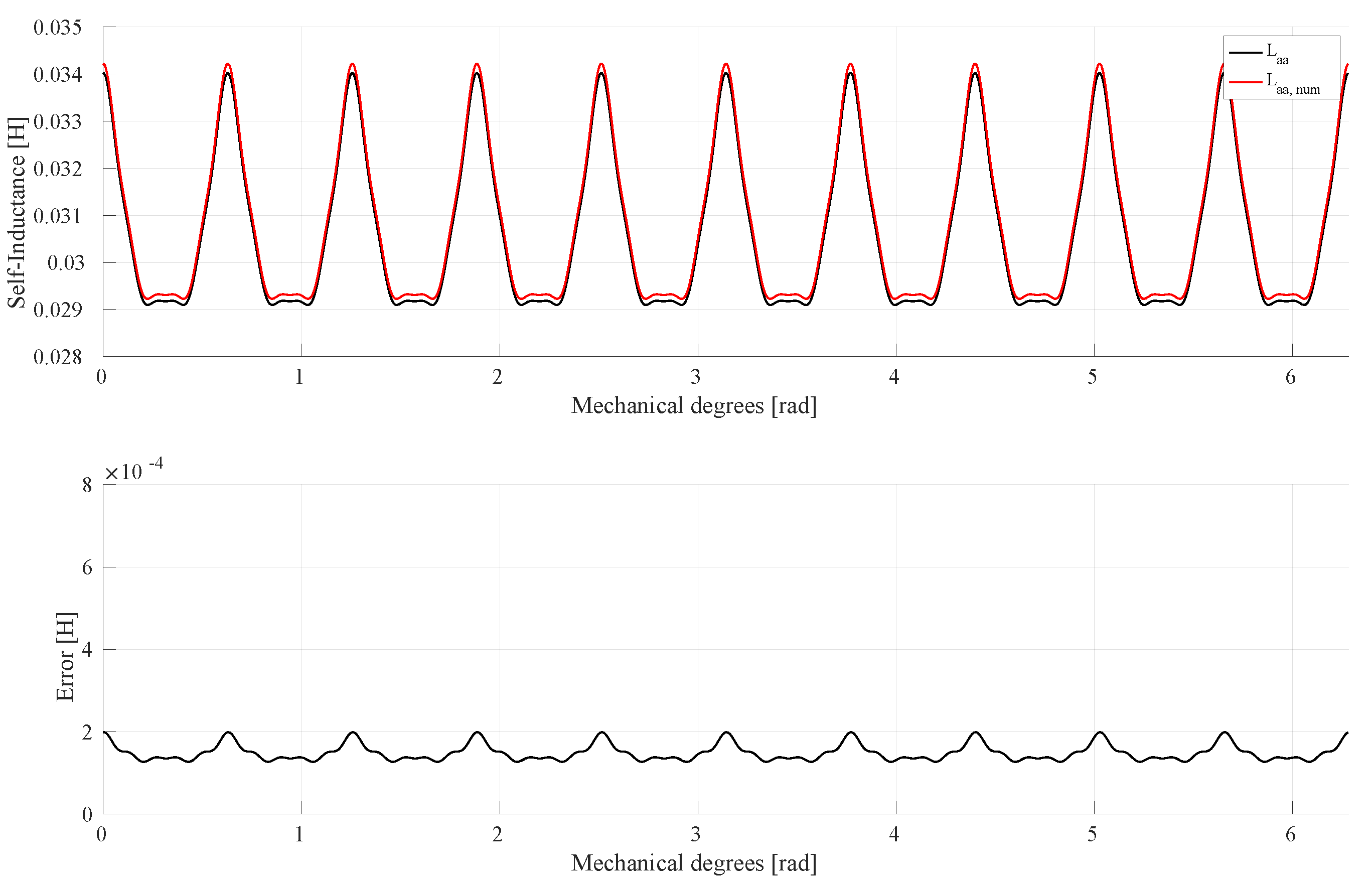
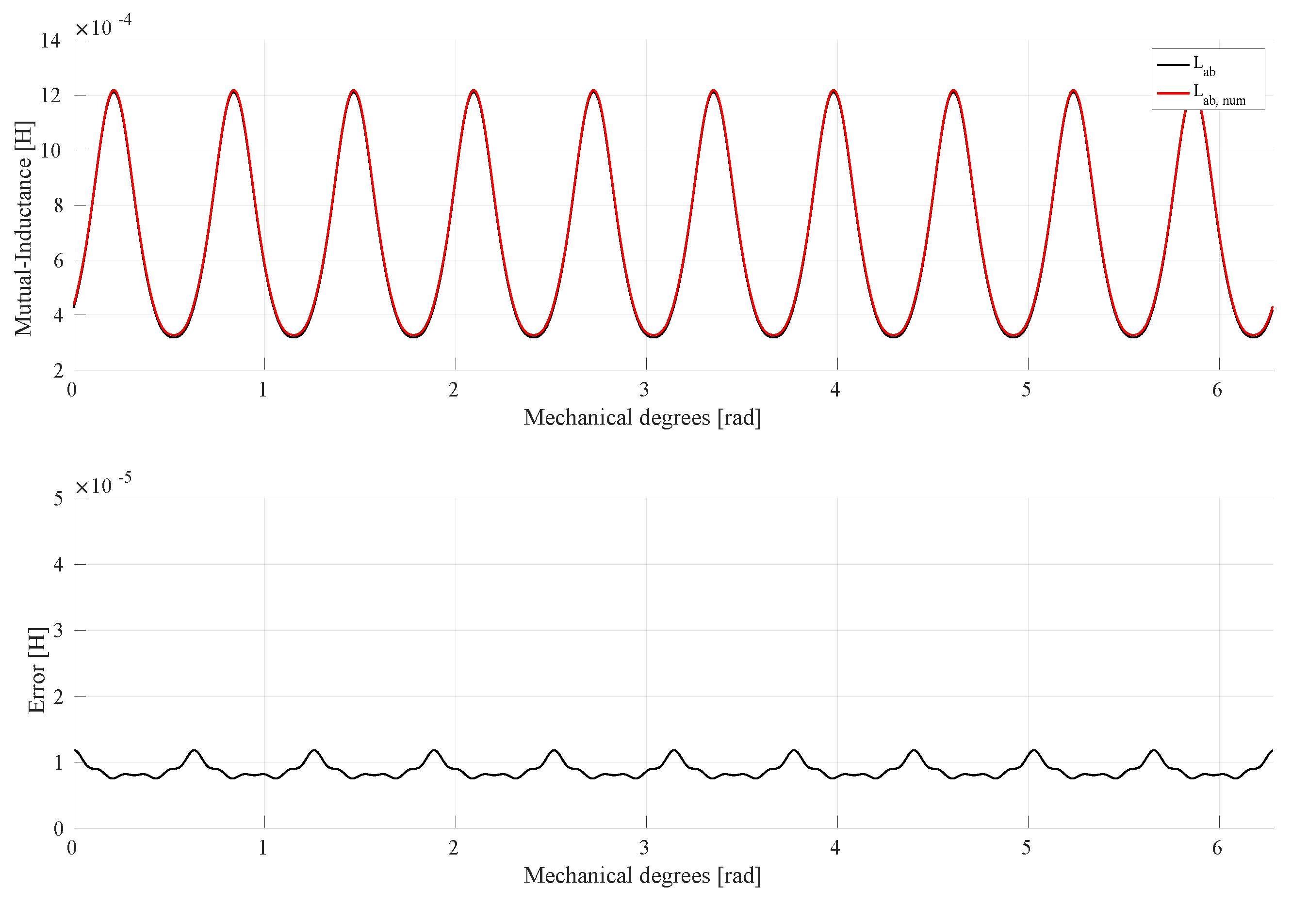
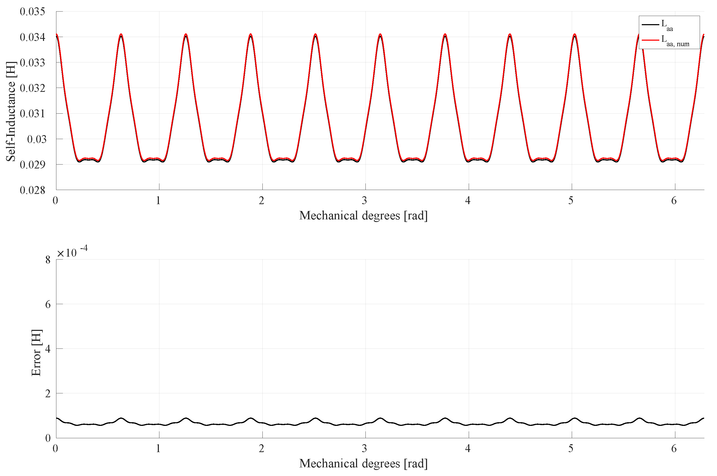
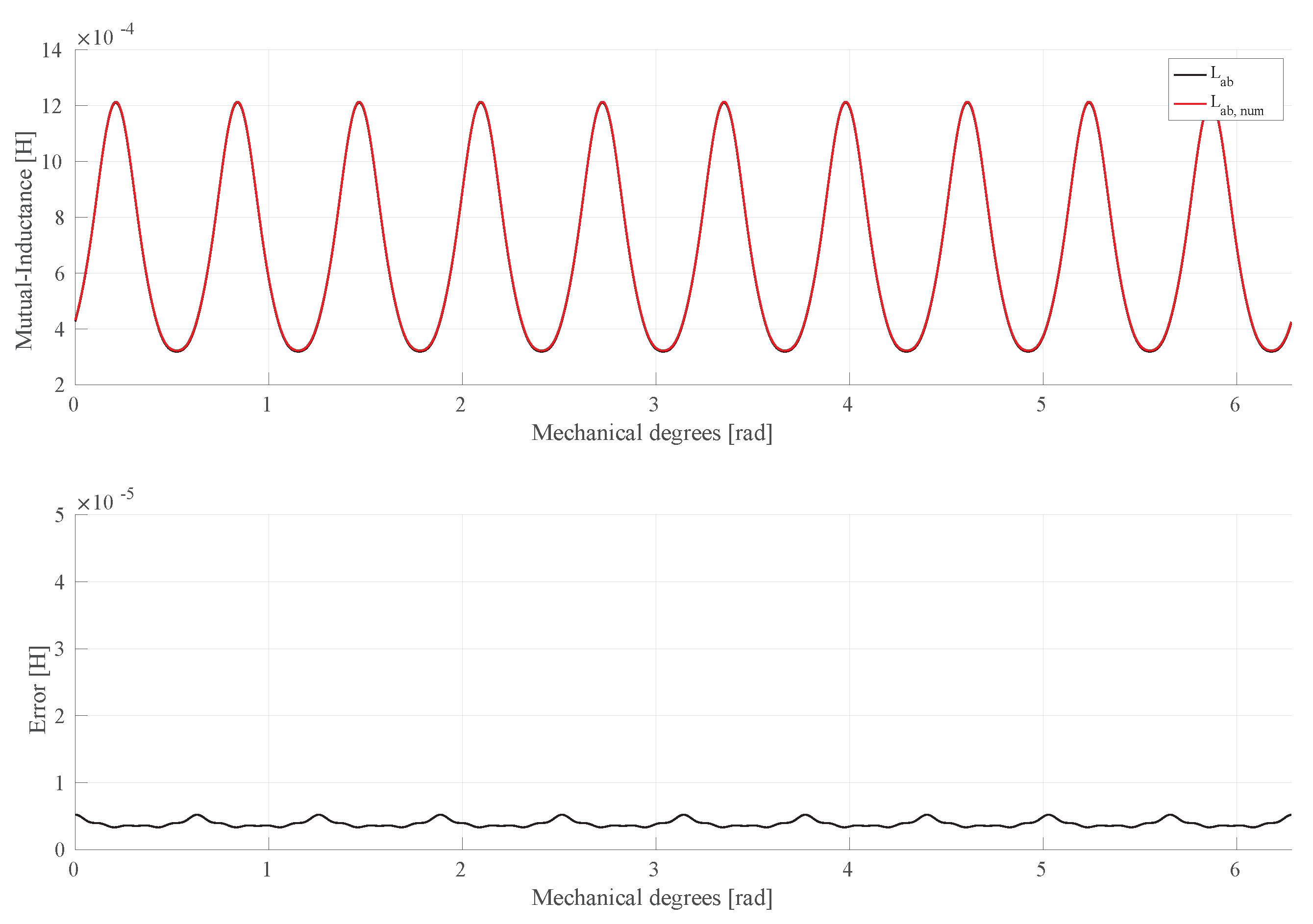
This work derives and presents an exact solution to the MWFA equation for PMSMs that highlights the harmonic content of the machine phase inductances in dependence of machine eccentricity. After introducing the MWFA formula and the mathematical expressions of each term, the exact solution is derived. Afterwards, validation is conducted by means of numerical simulations.

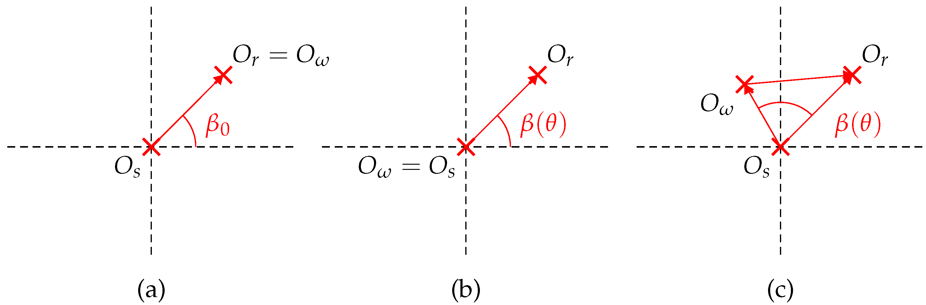
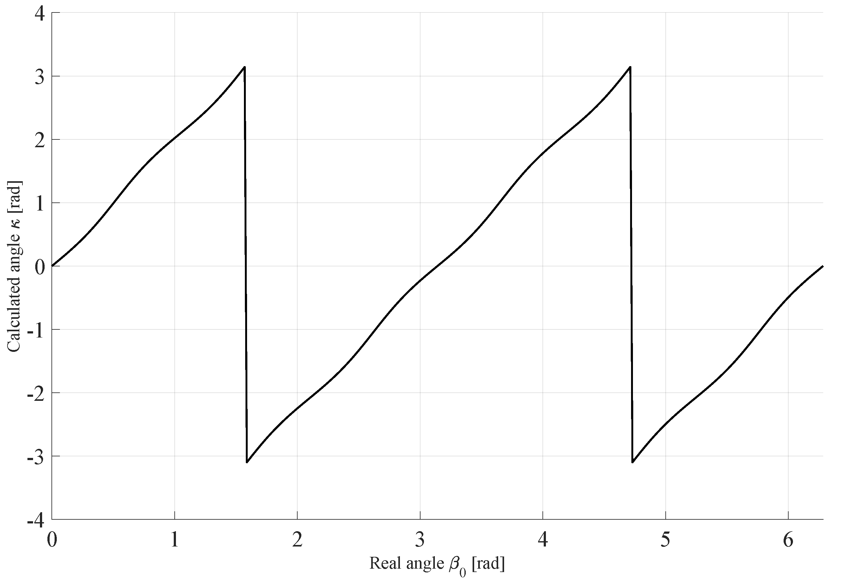
2. Eccentricity

Electrical machines are typically affected by eccentricity. As described in the Ref. [14], tolerances in manufacturing and assembly processes generally lead to eccentricities of 5–10% at the end of line of motor productions. Other sources of eccentricity include material fatigue, corrosion, non-isotropic mass distribution, and poor lubrication. in the Ref. [27], eccentricity is distinguished as three types: static eccentricity (SE), dynamic eccentricity (DE) and mixed eccentricity (ME). These three categories are schematized in Figure 2.

In the case of SE, the rotor symmetry center $O_r$ coincides with the rotor rotation center $O_{\omega }$, but not with the stator symmetry center $O_s$. This offset is constant regarding distance and angle in the stator reference frame. The degree of SE, ${\delta }_s$, is defined as

$${\delta }_s=\frac{\left|\overline{O_s{O}_{\omega }}\right|}{g_0},$$

(2)

where $g_0$ is the average air-gap length of the healthy machine. The minimum air-gap length is at the angle ${\beta }_0$. ${\delta }_s$ and the other degrees of eccentricity are limited to values between zero and one. If they are one, the air-gap is zero at ${\beta }_0$, which means that the stator and rotor are in contact.

DE is typically caused by an unbalanced machine: $O_{\omega }$ coincides with $O_s$, but not with $O_r$. This leads to a rotation of $O_r$ around $O_s$ in the stator reference frame according to the mechanical angle $\theta$. The non-uniform air-gap in the rotor reference frame translates into a rotation of the minimum air-gap length in the stator reference frame according to

$$\beta =\theta +{\beta }_0.$$

(3)

The degree of DE, ${\delta }_d$, is

$${\delta }_d=\frac{\left|\overline{O_{\omega }{O}_r}\right|}{g_0}.$$

(4)

ME is the combination of SE and DE. Neither $O_{\omega }$, $O_s$ nor $O_r$ are aligned. As defined in the Ref. [27], the degree of ME, ${\delta }_m$, and angle of the air-gap, $\beta$, changes with $\theta$ according to

$$\begin{array}{cc}\hfill {\delta }_m& =\frac{\left|\overline{O_s{O}_r}\right|}{g_0}=|\frac{\overline{O_s{O}_{\omega }}}{g_0}+\frac{\overline{O_{\omega }{O}_r}}{g_0}|=\sqrt{{\delta }_s^2+{\delta }_d^2+2{\delta }_s{\delta }_{d}cos\left(\theta \right)},\hfill \end{array}$$

(5)

$$\begin{array}{cc}\hfill \beta \left(\theta \right)& =atan\left(\frac{{\delta }_{d}sin\left(\theta \right)}{{\delta }_s+{\delta }_{d}cos\left(\theta \right)}\right)+{\beta }_0.\hfill \end{array}$$

(6)

It is easy to prove that ME describes SE and DE if only one of them is present, which is why ME will be used to describe eccentricity in a general way.

3. Derivation of the General Solution

In order to solve Equation (1), the contained functions have to be defined. In this work, the functions are approximated by even Fourier-series with an arbitrary number of harmonics, as highlighted in the Ref. [20].

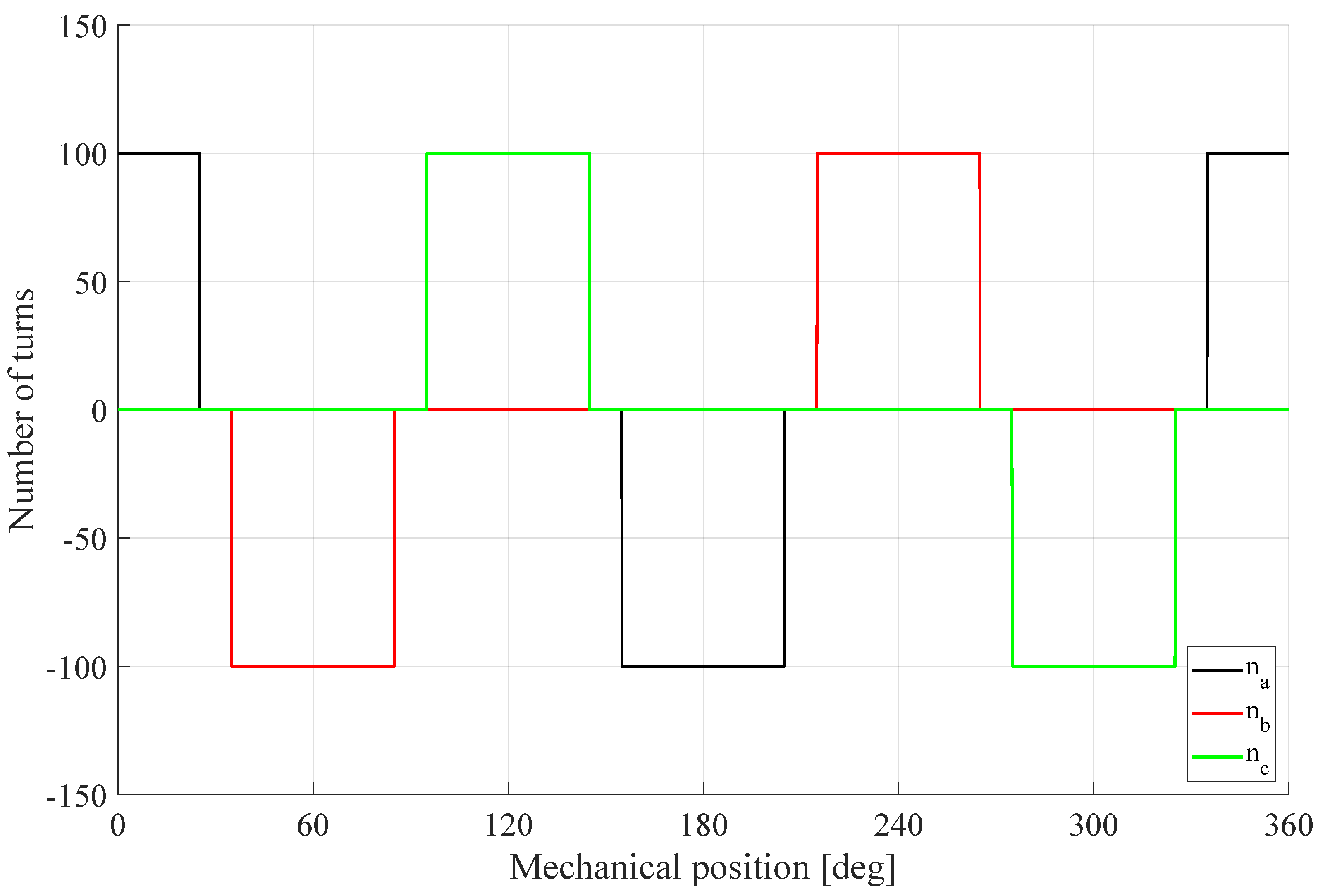
The turns function $n_x\left(\phi \right)$ describes the windings of the machine as the number of turns at every position $\phi$ in the stator reference frame. Depending on the direction of the current in the turn, it is counted as positive or negative. $n_x\left(\phi \right)$ is defined as

$$n_x\left(\phi \right)=\sum _{k=0}^{N_a}{A}_{k}cos\left(k(\phi +{\phi }_x)\right),$$

(7)

where $N_a$ is the number of harmonics considered, $A_k$ is the coefficient of the kth harmonic, and ${\phi }_x$ is the phase shift of phase x in the stator reference system. As $\phi$ is an arbitrary angle, any symmetric winding can be phase-shifted to be even. This allows the Fourier-series to only contain cosines.

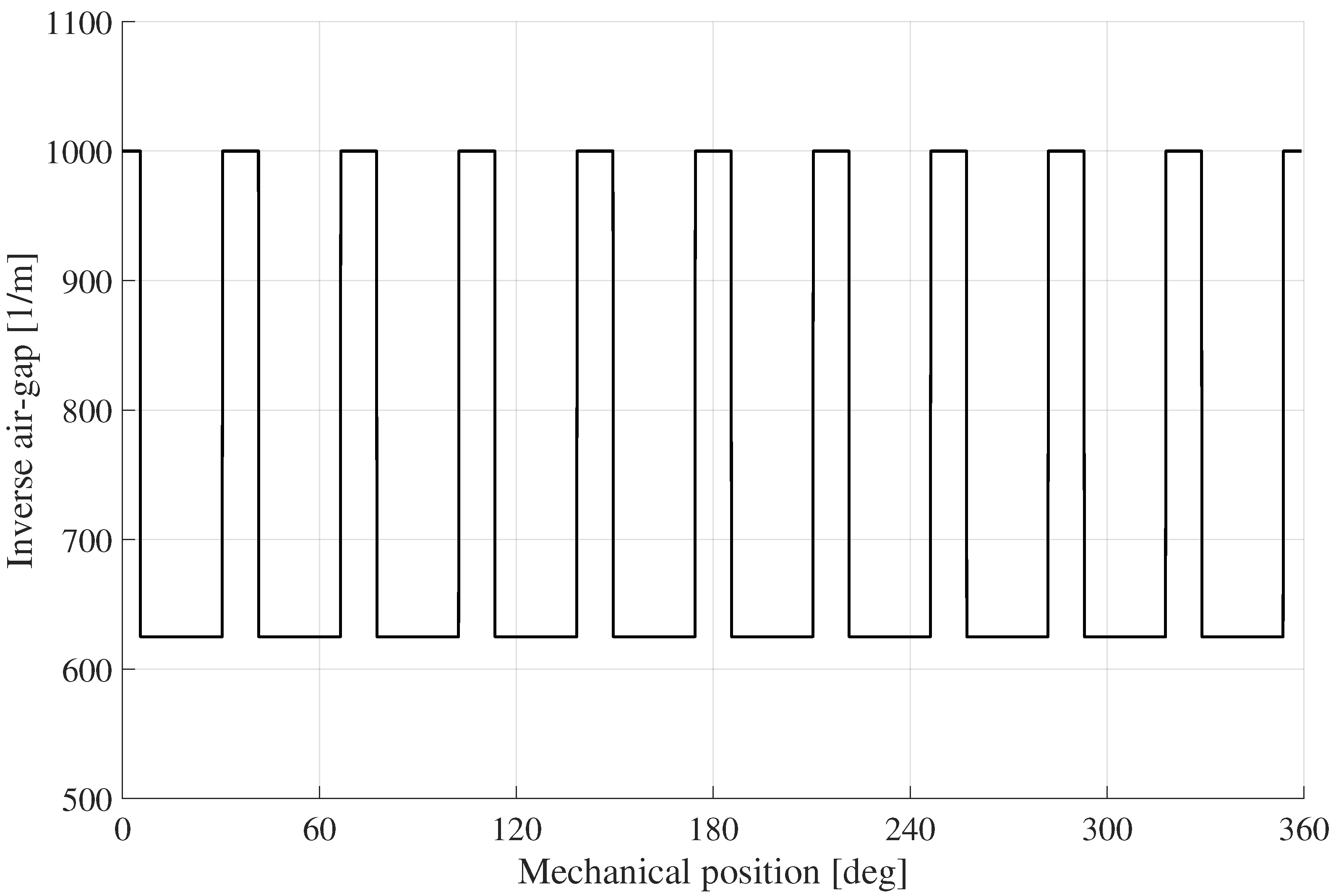
The inverse air-gap function $g^{-1}(\phi ,\theta )$ describes the inverse of the air-gap length between the stator and the rotor. It is highly dependent on the machine geometry and will change due to eccentricity. As the permeability of permanent magnets is close to the permeability of air, the air-gap includes any permanent magnet-filled slot. Its complete form is

$$\begin{array}{cc}\hfill g^{-1}(\phi ,\theta )=& {\overline{G}}_0+\Delta G+\Delta G_e=\hfill \\ \hfill & {\overline{G}}_0+\sum _{k=1}^{N_g}{G}_{2pk}cos\left(2pk(\phi -\theta )\right)+\sum _{t=1}^{N_e}{G}_{e,t}cos\left(t(\phi -\beta )\right).\hfill \end{array}$$

(8)

The inverse air-gap function consists of two parts: the healthy machine contributes a Fourier-series of the symmetric air-gap in the form of a mean value $G_0$ and even harmonics $\Delta G={\sum }_{k=1}^{N_g}{G}_{2pk}cos\left(2pk(\phi -\theta )\right)$, where $N_g$ is the number of harmonics considered, p is the number of pole pairs of the machine, and $G_{2pk}$ is the coefficient of the harmonic $2pk$. If the machine sustains eccentricity, the mean value $G_0$ of the air-gap changes according to

$$\overline{G_0}=\frac{G_0}{\sqrt{1-{\delta }_m^2}}.$$

(9)

If no eccentricity is present, this equation simplifies to ${\overline{G}}_0=G_0$. Eccentricity may also introduce $N_e$ additional harmonics $\Delta G_e={\sum }_{t=1}^{N_e}{G}_{e,t}cos\left(t(\phi -\beta )\right)$, where $G_{e,t}$ is the coefficient of the tth harmonic and, as shown in the Ref. [27], it is defined as

$$G_{e,t}=\overline{G_0}{\left(\frac{1-\sqrt{1-{\delta }_m^2}}{{\delta }_m}\right)}^t.$$

(10)

In the presence of eccentricity, some harmonics are considered both in the healthy machine formula, as well as in the eccentric one. This infers a change of harmonics existing in the healthy machine.

The modified winding function $N_x(\phi ,\theta )$, as introduced in the Ref. [20], is defined as

$$N_x(\phi ,\theta )=n_x\left(\phi \right)-\frac{1}{2\pi <g^{-1}(\phi ,\theta )>}{\int }_0^{2\pi }{n}_x\left(\phi \right)g^{-1}(\phi ,\theta )d\phi ,$$

(11)

with $<g^{-1}(\phi ,\theta )>$ being the mean value of the inverse air-gap function $\overline{G_0}$.

Inserting $N_x(\phi ,\theta )$ into Equation (1) leads to

$$L_{xy}={\mu }_{0}rl{\int }_0^{2\pi }\left[n_y-\frac{1}{2\pi {\overline{G}}_0}{\int }_0^{2\pi }{n}_y{g}^{-1}d\phi \right]n_x{g}^{-1}d\phi ,$$

(12)

which can be extended into a sum of integrals by inserting Equation (8)

$$\begin{array}{cc}\hfill L_{xy}=& M{\int }_0^{2\pi }\left[n_y-\frac{1}{2\pi {\overline{G}}_0}{\int }_0^{2\pi }{n}_y{\overline{G}}_0\phi \right]n_x{\overline{G}}_{0}d\phi +\hfill \\ \hfill & M{\int }_0^{2\pi }\left[-\frac{1}{2\pi {\overline{G}}_0}{\int }_0^{2\pi }{n}_y\Delta Gd\phi \right]n_x{\overline{G}}_{0}d\phi +\hfill \\ \hfill & M{\int }_0^{2\pi }\left[n_y-\frac{1}{2\pi {\overline{G}}_0}{\int }_0^{2\pi }{n}_y{\overline{G}}_0\phi \right]n_x\Delta Gd\phi +\hfill \\ \hfill & M{\int }_0^{2\pi }\left[-\frac{1}{2\pi {\overline{G}}_0}{\int }_0^{2\pi }{n}_y\Delta Gd\phi \right]n_x\Delta Gd\phi +\hfill \\ \hfill & M{\int }_0^{2\pi }\left[-\frac{1}{2\pi {\overline{G}}_0}{\int }_0^{2\pi }{n}_y\Delta G_{e}d\phi \right]n_x({\overline{G}}_0+\Delta G)d\phi +\hfill \\ \hfill & M{\int }_0^{2\pi }{n}_y{n}_x\Delta G_{e}d\phi +\hfill \\ \hfill & M{\int }_0^{2\pi }\left[-\frac{1}{2\pi {\overline{G}}_0}{\int }_0^{2\pi }{n}_y({\overline{G}}_0+\Delta G)d\phi \right]n_x\Delta G_{e}d\phi +\hfill \\ \hfill & M{\int }_0^{2\pi }\left[-\frac{1}{2\pi {\overline{G}}_0}{\int }_0^{2\pi }{n}_y\Delta G_{e}d\phi \right]n_x\Delta G_{e}d\phi =\hfill \\ \hfill & \left(I\right)+\left(II\right)+\left(III\right)+\left(IV\right)+\left(V\right)+\left(VI\right)+\left(VII\right)+\left(VIII\right),\hfill \end{array}$$

(13)

where $M={\mu }_{0}rl$. The addends $\left(I\right)$ to $\left(VIII\right)$ will be examined separately for readability purposes.

Inserting $n_x\left(\phi \right)$ into the first equation results in

$$\begin{array}{cc}\hfill \left(I\right)=& M{\int }_0^{2\pi }\left[\sum _{k=0}^{N_a}{A}_{k}cos\left(k(\phi +{\phi }_y)\right)-\frac{1}{2\pi {\overline{G}}_0}{\int }_0^{2\pi }\sum _{k=0}^{N_a}{A}_{k}cos\left(k(\phi +{\phi }_y)\right){\overline{G}}_{0}d\phi \right]·\hfill \\ \hfill & \sum _{k=0}^{N_a}{A}_{k}cos\left(k(\phi +{\phi }_x)\right){\overline{G}}_{0}d\phi =\hfill \\ \hfill & M{\overline{G}}_0{\int }_0^{2\pi }\left[\sum _{k=0}^{N_a}{A}_{k}cos\left(k(\phi +{\phi }_y)\right)-\frac{1}{2\pi }{\int }_0^{2\pi }\sum _{k=0}^{N_a}{A}_{k}cos\left(k(\phi +{\phi }_y)\right)d\phi \right]·\hfill \\ \hfill & \sum _{k=0}^{N_a}{A}_{k}cos\left(k(\phi +{\phi }_x)\right)d\phi =\hfill \\ \hfill & M{\overline{G}}_0{\int }_0^{2\pi }\left[\sum _{k=0}^{N_a}{A}_{k}cos\left(k(\phi +{\phi }_y)\right)-A_0\right]\sum _{k=0}^{N_a}{A}_{k}cos\left(k(\phi +{\phi }_x)\right)d\phi =\hfill \\ \hfill & M{\overline{G}}_0{\int }_0^{2\pi }\sum _{k=1}^{N_a}{A}_{k}cos\left(k(\phi +{\phi }_y)\right)\sum _{k=0}^{N_a}{A}_{k}cos\left(k(\phi +{\phi }_x)\right)d\phi =\hfill \\ \hfill & M{\overline{G}}_0\pi \sum _{k=1}^{N_a}{A}_k^{2}cos\left(k({\phi }_x-{\phi }_y)\right).\hfill \end{array}$$

(14)

This part only exhibits a mean value and describes the inductance of a healthy SPMSM. Using the assumptions introduced, the air-gap of a healthy SPMSM is constant. In the general equation, this can be achieved with $g^{-1}(\phi ,\theta )=G_0$, which removes all effects of the remaining terms $II$–$VIII$. An eccentric SPMSM can also be described on its own, although the derivation of the expression is not shown here as the general expression is sufficient to describe both SPMSMs and IPMSMs.

Examining the next part leads to

$$\begin{array}{cc}\hfill \left(II\right)=& M{\int }_0^{2\pi }\left[-\frac{1}{2\pi {\overline{G}}_0}{\int }_0^{2\pi }\sum _{k=0}^{N_a}{A}_{k}cos\left(k(\phi +{\phi }_y)\right)\sum _{t=1}^{N_g}{G}_{2pt}cos\left(2pt(\phi -\theta )\right)d\phi \right]·\hfill \\ \hfill & \sum _{k=0}^{N_a}{A}_{k}cos\left(k(\phi +{\phi }_x)\right){\overline{G}}_{0}d\phi =\hfill \\ \hfill & -\frac{M}{2\pi }{\int }_0^{2\pi }\sum _{k=0}^{N_a}{A}_{k}cos\left(k(\phi +{\phi }_y)\right)\sum _{t=1}^{N_g}{G}_{2pt}cos\left(2pt(\phi -\theta )\right)d\phi ·\hfill \\ \hfill & {\int }_0^{2\pi }\sum _{k=0}^{N_a}{A}_{k}cos\left(k(\phi +{\phi }_x)\right)d\phi =\hfill \\ \hfill & -\frac{M}{2\pi }\sum _{t=1}^{N_g}\pi A_{2pt}{G}_{2pt}cos\left(2pt(\theta +{\phi }_y)\right)2\pi A_0=\hfill \\ \hfill & -M{A}_0\pi \sum _{k=1}^{N_g}{A}_{2pt}{G}_{2pt}cos\left(2pt(\theta +{\phi }_y)\right).\hfill \end{array}$$

(15)

When multiplying the sums inside an integral, the highest harmonic present is defined by the smaller number between $N_a$ and $2p{N}_g$. This is due to all higher harmonics created containing $\phi$. As $\phi$ is the integration variable and the integration is always performed between 0 and $2\pi$, they have no contribution on the final result. Choosing $N_g$ for the resulting sum is arbitrary, as the amplitude $A_k$ of harmonics higher than $N_a$ are considered zero in $n_x\left(\phi \right)$, and therefore, in the resulting sum too. This property is considered true for all coefficients outside their defined range. Although this leads to unnecessary calculations when applying these equations, it greatly reduces their complexity without changing the result. A possibility to avoid these calculation steps is to check $N_a$, $N_g$, and $N_e$ and only perform the calculation if all necessary coefficients are defined.

Part $\left(III\right)$ can be transformed to

$$\begin{array}{cc}\hfill \left(III\right)=& M{\int }_0^{2\pi }\left[\sum _{k=0}^{N_a}{A}_{k}cos\left(k(\phi +{\phi }_y)\right)-\frac{1}{2\pi {\overline{G}}_0}{\int }_0^{2\pi }\sum _{k=0}^{N_a}{A}_{k}cos\left(k(\phi +{\phi }_y)\right){\overline{G}}_{0}d\phi \right]·\hfill \\ \hfill & \sum _{k=0}^{N_a}{A}_{k}cos\left(k(\phi +{\phi }_x)\right)\sum _{t=1}^{N_g}{G}_{2pt}cos\left(2pt(\phi -\theta )\right)d\phi =\hfill \\ \hfill & M{\int }_0^{2\pi }\left[\sum _{k=0}^{N_a}{A}_{k}cos\left(k(\phi +{\phi }_y)\right)-A_0\right]\sum _{k=0}^{N_a}{A}_{k}cos\left(k(\phi +{\phi }_x)\right)·\hfill \\ \hfill & \sum _{t=1}^{N_g}{G}_{2pt}cos\left(2pt(\phi -\theta )\right)d\phi =\hfill \\ \hfill & M{\int }_0^{2\pi }\sum _{k=1}^{N_a}{A}_{k}cos\left(k(\phi +{\phi }_y)\right)\sum _{k=0}^{N_a}{A}_{k}cos\left(k(\phi +{\phi }_x)\right)·\hfill \\ \hfill & \sum _{t=1}^{N_g}{G}_{2pt}cos\left(2pt(\phi -\theta )\right)d\phi .\hfill \end{array}$$

(16)

Differently from the other cases, here the product of three sums is present. Nevertheless, the product of the sums of the turns functions can be proven to reduce to:

$$\begin{array}{cc}\hfill & \sum _{k=1}^{N_a}{A}_{k}cos\left(k(\phi +{\phi }_y)\right)\sum _{k=0}^{N_a}{A}_{k}cos\left(k(\phi +{\phi }_x)\right)=\hfill \\ \hfill & A_0\sum _{k=1}^{N_a}{A}_{k}cos\left(k(\phi +{\phi }_y)\right)+\sum _{k=1}^{N_a}\frac{1}{2}{A}_k^{2}cos\left(k({\phi }_x-{\phi }_y)\right)+\hfill \\ \hfill & \frac{1}{2}\sum _{k=1}^{2N_a}\left[\sum _{t=1}^{N_a}{A}_t{A}_{k+t}cos(k\phi +(k+t){\phi }_x-t{\phi }_y)+\sum _{\begin{array}{c}t=1\\ t\ne k\end{array}}^{N_a}{A}_t{A}_{|t-k|}cos(k\phi +(k-t){\phi }_x+t{\phi }_y)\right].\hfill \end{array}$$

(17)

This formulation allows to bring the result into the more convenient following form:

$$L_{xy}=L_0+\sum _{k=1}^{\infty }{N}_{k}cos\left(k(\theta -{\alpha }_k)\right).$$

(18)

Inserting Equation (17) into Equation (16) results in

$$\begin{array}{cc}\hfill \left(III\right)=& M{\int }_0^{2\pi }{A}_0\sum _{k=1}^{N_a}{A}_{k}cos\left(k(\phi +{\phi }_y)\right)\sum _{t=1}^{N_g}{G}_{2pt}cos\left(2pt(\phi -\theta )\right)d\phi +\hfill \\ \hfill & \frac{M}{2}\sum _{k=1}^{N_a}{A}_k^{2}cos\left(k({\phi }_x-{\phi }_y)\right){\int }_0^{2\pi }\sum _{t=1}^{N_g}{G}_{2pt}cos\left(2pt(\phi -\theta )\right)d\phi +\hfill \\ \hfill & \frac{M}{2}{\int }_0^{2\pi }\sum _{k=1}^{2N_a}[\sum _{t=1}^{N_a}{A}_t{A}_{k+t}cos(k\phi +(k+t){\phi }_x-t{\phi }_y)+\hfill \\ \hfill & \sum _{\begin{array}{c}t=1\\ t\ne k\end{array}}^{N_a}{A}_t{A}_{|t-k|}cos(k\phi +(k-t){\phi }_x+t{\phi }_y)]·\hfill \\ \hfill & \sum _{t=1}^{N_g}{G}_{2pt}cos\left(2pt(\phi -\theta )\right)d\phi =\hfill \\ \hfill & M{A}_0\pi \sum _{k=1}^{N_g}{A}_{2pk}{G}_{2pk}cos\left(2pk(\theta +{\phi }_y)\right)+\hfill \\ \hfill & \frac{M}{2}{\int }_0^{2\pi }\sum _{k=1}^{2N_a}{N}_{k}cos(k\phi -{\alpha }_k)\sum _{t=1}^{N_g}{G}_{2pt}cos\left(2pt(\phi -\theta )\right)d\phi =\hfill \\ \hfill & M{A}_0\pi \sum _{k=1}^{N_g}{A}_{2pk}{G}_{2pk}cos\left(2pk(\theta +{\phi }_y)\right)+\hfill \\ \hfill & \frac{M\pi }{2}\sum _{k=1}^{N_g}{N}_{2pk}{G}_{2pk}cos(2pk\theta -{\alpha }_{2pk}).\hfill \end{array}$$

(19)

$N_k$ and ${\alpha }_k$ are introduced for notation purposes. Their full expressions can be found in Appendix A.

The notation introduced in Equation (17) is used to solve part $\left(IV\right)$ too:

$$\begin{array}{cc}\hfill \left(IV\right)=& M{\int }_0^{2\pi }\left[-\frac{1}{2\pi {\overline{G}}_0}{\int }_0^{2\pi }\sum _{k=0}^{N_a}{A}_{k}cos\left(k(\phi +{\phi }_y)\right)\sum _{t=1}^{N_g}{G}_{2pt}cos\left(2pt(\phi -\theta )\right)d\phi \right]·\hfill \\ \hfill & \sum _{k=0}^{N_a}{A}_{k}cos\left(k(\phi +{\phi }_x)\right)\sum _{t=1}^{N_g}{G}_{2pt}cos\left(2pt(\phi -\theta )\right)d\phi =\hfill \\ \hfill & -\frac{M}{2\pi {\overline{G}}_0}{\int }_0^{2\pi }\sum _{k=0}^{N_a}{A}_{k}cos\left(k(\phi +{\phi }_y)\right)\sum _{t=1}^{N_g}{G}_{2pt}cos\left(2pt(\phi -\theta )\right)d\phi ·\hfill \\ \hfill & {\int }_0^{2\pi }\sum _{k=0}^{N_a}{A}_{k}cos\left(k(\phi +{\phi }_x)\right)\sum _{t=1}^{N_g}{G}_{2pt}cos\left(2pt(\phi -\theta )\right)d\phi =\hfill \\ \hfill & -\frac{M\pi }{2{\overline{G}}_0}\sum _{k=1}^{N_g}{A}_{2pk}{G}_{2pk}cos\left(2pk(\theta +{\phi }_y)\right)\sum _{t=1}^{N_g}{A}_{2pt}{G}_{2pt}cos\left(2pt(\theta +{\phi }_x)\right)=\hfill \\ \hfill & -\frac{M\pi }{4{\overline{G}}_0}[\sum _{k=1}^{N_g}{A}_{2pk}^2{G}_{2pk}^{2}cos\left(2pk({\phi }_x-{\phi }_y)\right)+\hfill \\ \hfill & \sum _{k=1}^{2N_g}[\sum _{t=1}^{N_g}{A}_{2pt}{G}_{2pt}{A}_{2p(k+t)}{G}_{2p(k+t)}cos\left(2p(k\theta +(k+t){\phi }_x-t{\phi }_y)\right)+\hfill \\ \hfill & \sum _{\begin{array}{c}t=1\\ t\ne k\end{array}}^{N_g}{A}_{2pt}{G}_{2pt}{A}_{2p|t-k|}{G}_{2p|t-k|}cos\left(2p(k\theta +(k-t){\phi }_x+t{\phi }_y)\right)]].\hfill \end{array}$$

(20)

A highly interesting observation is the introduction of harmonics up to $4p{N}_g$, which is twice as high as the number of harmonics considered in the initial function. The effective highest harmonic also depends on $N_a$, as harmonics only have a non-zero amplitude if both the turns and the air-gap function coefficients are non-zero, but if $N_a$ is high enough, this statement is true.

All addends until this point have not contained eccentricity apart from the change in the mean value of the inverse air-gap. Therefore, replacing this value with the one of the healthy machine describes the inductance without eccentricity. Combining the partial results and rearranging them leads to

$$L_{xy}=L_{0,h}+\sum _{k=1}^{2N_g}{\overline{N}}_{2pk}cos(2pk\theta -{\overline{\alpha }}_{2pk}),$$

(21)

where $L_{0,h}$ is the mean value of the inductance and the harmonics are described by the coefficient ${\overline{N}}_{2pk}$ and phase shift ${\overline{\alpha }}_{2pk}$. The full expression of these variables can be found in Appendix A. This form clearly shows that, given the assumptions made, all present harmonics in a healthy machine are even. As the mechanical angle $\theta$ always appears in connection with $2p$, the harmonics are only referring to the electrical period.

The first term that includes eccentricity can be rewritten as

$$\begin{array}{cc}\hfill \left(V\right)=& M{\int }_0^{2\pi }\left[-\frac{1}{2\pi {\overline{G}}_0}{\int }_0^{2\pi }\sum _{k=0}^{N_a}{A}_{k}cos\left(k(\phi +{\phi }_y)\right)\sum _{t=1}^{N_e}{G}_{e,t}cos\left(k(\phi -\beta )\right)d\phi \right]·\hfill \\ \hfill & \sum _{k=0}^{N_a}{A}_{k}cos\left(k(\phi +{\phi }_x)\right)({\overline{G}}_0+\sum _{t=1}^{N_g}{G}_{2pt}cos\left(2pt(\phi -\theta )\right))d\phi =\hfill \\ \hfill & -\frac{M}{2\pi {\overline{G}}_0}{\int }_0^{2\pi }\sum _{k=0}^{N_a}{A}_{k}cos\left(k(\phi +{\phi }_y)\right)\sum _{t=1}^{N_e}{G}_{e,t}cos\left(k(\phi -\beta )\right)d\phi ·\hfill \\ \hfill & {\int }_0^{2\pi }\sum _{k=0}^{N_a}{A}_{k}cos\left(k(\phi +{\phi }_x)\right)({\overline{G}}_0+\sum _{t=1}^{N_g}{G}_{2pt}cos\left(2pt(\phi -\theta )\right))d\phi =\hfill \\ \hfill & -\frac{M}{2\pi {\overline{G}}_0}\pi \sum _{k=1}^{N_e}{A}_k{G}_{e,k}cos\left(k(\beta +{\phi }_y)\right)\left[2\pi {\overline{G}}_0{A}_0+\pi \sum _{t=1}^{N_g}{A}_{2pt}{G}_{2pt}cos\left(2pt(\theta +{\phi }_x)\right)\right]=\hfill \\ \hfill & M\pi A_0\sum _{k=1}^{N_e}{A}_k{G}_{e,k}cos\left(k(\beta +{\phi }_y)\right)-\hfill \\ \hfill & \frac{M\pi }{2{\overline{G}}_0}\sum _{k=1}^{N_e}{A}_k{G}_{e,k}cos\left(k(\beta +{\phi }_y)\right)\sum _{t=1}^{N_g}{A}_{2pt}{G}_{2pt}cos\left(2pt(\theta +{\phi }_x)\right).\hfill \end{array}$$

(22)

The general solution of part $\left(V\right)$ still contains a product of two sums. As $\theta$ and $\beta$ are not equal at all times, Equation (17) cannot be applied. This problem may simplify depending on the type of eccentricity present in the machine, which will be presented at a later point. If the solution cannot be simplified, the product of these sums represents harmonics around the already existing electrical ones introduced by eccentricity. Once again, the choice of $N_e$ instead of $N_a$ is arbitrary, as the coefficients of harmonics higher than $N_a$ are zero.

Equation (17) is applied to solve part $\left(VI\right)$:

$$\begin{array}{cc}\hfill \left(VI\right)=& M{\int }_0^{2\pi }\sum _{k=0}^{N_a}{A}_{k}cos\left(k(\phi +{\phi }_y)\right)\sum _{k=0}^{N_a}{A}_{k}cos\left(k(\phi +{\phi }_x)\right)\sum _{t=1}^{N_e}{G}_{e,t}cos\left(k(\phi -\beta )\right)d\phi =\hfill \\ \hfill & M{A}_0\pi \sum _{k=1}^{N_e}{A}_k{G}_{2,k}\left[cos\left(k(\beta +{\phi }_x)\right)+cos\left(k(\beta +{\phi }_y)\right)\right]+\hfill \\ \hfill & M{\int }_0^{2\pi }\sum _{k=0}^{2N_a}{N}_{k}cos(k\phi -{\alpha }_k)\sum _{t=1}^{N_e}{G}_{e,t}cos\left(k(\phi -\beta )\right)d\phi =\hfill \\ \hfill & M{A}_0\pi \sum _{k=1}^{N_e}{A}_k{G}_{2,k}\left[cos\left(k(\beta +{\phi }_x)\right)+cos\left(k(\beta +{\phi }_y)\right)\right]+M\pi \sum _{k=1}^{N_e}{N}_k{G}_{e,k}cos(k\beta -{\alpha }_k).\hfill \end{array}$$

(23)

Part $\left(VII\right)$ is very similar to part $\left(V\right)$. Indeed, the only difference is a switch of $n_x$ and $n_y$. The solution of $\left(VII\right)$ is, therefore, acquired by a minor change of Equation (22), which results in

$$\begin{array}{cc}\hfill \left(VII\right)=& M\pi A_0\sum _{k=1}^{N_e}{A}_k{G}_{e,k}cos\left(k(\beta +{\phi }_x)\right)-\hfill \\ \hfill & \frac{M\pi }{2{\overline{G}}_0}\sum _{k=1}^{N_e}{A}_k{G}_{e,k}cos\left(k(\beta +{\phi }_x)\right)\sum _{t=1}^{N_g}{A}_{2pt}{G}_{2pt}cos\left(2pt(\theta +{\phi }_y)\right).\hfill \end{array}$$

(24)

The last part requires the usage of Equation (17), which leads to

$$\begin{array}{cc}\hfill \left(VIII\right)=& M{\int }_0^{2\pi }\left[-\frac{1}{2\pi {\overline{G}}_0}{\int }_0^{2\pi }\sum _{k=0}^{N_a}{A}_{k}cos\left(k(\phi +{\phi }_y)\right)\sum _{t=1}^{N_e}{G}_{e,t}cos\left(k(\phi -\beta )\right)d\phi \right]·\hfill \\ \hfill & \sum _{k=0}^{N_a}{A}_{k}cos\left(k(\phi +{\phi }_x)\right)\sum _{t=1}^{N_e}{G}_{e,t}cos\left(k(\phi -\beta )\right)d\phi =\hfill \\ \hfill & -\frac{M}{2\pi {\overline{G}}_0}{\int }_0^{2\pi }\sum _{k=0}^{N_a}{A}_{k}cos\left(k(\phi +{\phi }_y)\right)\sum _{t=1}^{N_e}{G}_{e,t}cos\left(k(\phi -\beta )\right)d\phi ·\hfill \\ \hfill & {\int }_0^{2\pi }\sum _{k=0}^{N_a}{A}_{k}cos\left(k(\phi +{\phi }_x)\right)\sum _{t=1}^{N_e}{G}_{e,t}cos\left(k(\phi -\beta )\right)d\phi =\hfill \\ \hfill & -\frac{M\pi }{2{\overline{G}}_0}\sum _{k=1}^{N_e}{A}_k{G}_{e,k}cos\left(k(\beta +{\phi }_y)\right)\sum _{t=1}^{N_e}{A}_t{G}_{e,t}cos\left(t(\beta +{\phi }_x)\right)=\hfill \\ \hfill & -\frac{M\pi }{4{\overline{G}}_0}[\sum _{k=1}^{N_e}{A}_k^2{G}_{e,k}^{2}cos\left(k({\phi }_x-{\phi }_y)\right)+\hfill \\ \hfill & \sum _{k=1}^{2N_e}[\sum _{t=1}^{N_e}{A}_t{G}_{e,t}{A}_{t+k}{G}_{e,t+k}cos(k\beta +(k+t){\phi }_x-t{\phi }_y)+\hfill \\ \hfill & \sum _{\begin{array}{c}t=1\\ t\ne k\end{array}}^{N_e}{A}_t{G}_{e,t}{A}_{|t-k|}{G}_{e,|t-k|}cos(k\beta +(k-t){\phi }_x+t{\phi }_y)]].\hfill \end{array}$$

(25)

Finally, combining all the addends $\left(I\right)$ to $\left(VIII\right)$ and rearranging the solution results in

$$\begin{array}{cc}\hfill L_{xy}\left(\theta \right)=& L_0+L_{c,0}+L_{e,0}+\sum _{k=1}^{2N_g}[{\overline{N}}_{2pk}cos(2pk\theta -{\overline{\alpha }}_{2pk})+{\overline{N}}_{c,2pk}cos(2pk\theta -{\overline{\alpha }}_{c,2pk})]+\hfill \\ \hfill & \sum _{k=1}^{N_e}M\pi N_k{G}_{e,k}cos(k\beta -{\alpha }_k)+\sum _{k=1}^{2N_e}{\overline{M}}_{k}cos(k\beta -{\overline{\beta }}_k)-\hfill \\ \hfill & \frac{M\pi }{2{\overline{G}}_0}[\sum _{k=1}^{N_e}{A}_k{G}_{e,k}cos\left(k(\beta +{\phi }_x)\right)\sum _{t=1}^{N_g}{G}_{2pt}{A}_{2pt}cos\left(2pt(\theta +{\phi }_y)\right)+\hfill \\ \hfill & \sum _{k=1}^{N_e}{A}_k{G}_{e,k}cos\left(k(\beta +{\phi }_y)\right)\sum _{t=1}^{N_g}{G}_{2pt}{A}_{2pt}cos\left(2pt(\theta +{\phi }_x)\right)].\hfill \end{array}$$

(26)

This equation could be expressed in a more compact form. Nevertheless, it is chosen in order to illustrate the change in inductance due to eccentricity. $L_0$ is the mean inductance of the healthy machine. This mean value is changed due to the replacement of $G_0$ with ${\overline{G}}_0$, which is represented by the correction $L_{c,0}$. An independent mean value due to eccentricity is introduced with $L_{e,0}$. The existing harmonics, as employed in Equation (21), are corrected using ${\overline{N}}_{c,2pk}$ and ${\overline{\alpha }}_{c,2pk}$. The next two addends are, in the case of DE and ME, additional harmonics introduced due to eccentricity. These harmonics are directly linked to the mechanical angle $\theta$ without the number of pole pairs p. In the case of SE, these terms contribute to the mean value. ${\overline{M}}_k$, ${\overline{\beta }}_k$ and all other introduced variables can be found in Appendix A. The last part of Equation (26) is the aforementioned product of two sums, which, determined by the type of eccentricity, introduces additional harmonics.

4. Solutions for Special Cases

During the derivation of the general solution Equation (26), some parts were mentioned to differ depending on the type of eccentricity. Therefore, it is of interest to extract and examine separate solutions for the different types of eccentricity. Their derivation is not presented here, as it only consists of inserting $\beta$ and rearranging the equation in a clearer manner.

Inserting SE into Equation (26) simplifies the result to

$$L_{xy}=L_{se,0}+\sum _{k=1}^{2N_g}{K}_{se,2pk}cos(2pk\theta -{\alpha }_{se,2pk}),$$

(27)

where

$$L_{se,0}=L_0+L_{c,0}+L_{e,0}+L_{s,0},$$

(28)

and $L_{s,0}$ is an additional addend to the mean inductance only present under SE conditions. The full expressions of $L_{s,0}$, $K_{se,2pk}$, and ${\alpha }_{se,2pk}$ can be found in Appendix A.

Equation (27) clearly shows that SE only changes already existing features of the healthy machine and does not introduce further harmonics. This behavior is also supported by the harmonic content of the initial Equation (1) with and without SE, as shown in Figure 3.

In the case of DE, Equation (26) can be rearranged to

$$\begin{array}{cc}\hfill L_{xy}& =L_{de,0}+\sum _{k=1}^{2N_g}{\overline{N}}_{e,2pk}cos(2pk\theta -{\overline{\alpha }}_{e,2pk})+\sum _{k=1}^{2N_e}{M}_{de,k}cos(k\theta -{\beta }_{de,k})+\hfill \\ \hfill & \sum _{k=1}^{N_e}\sum _{t=1}^{N_g}\left[R_{k,2pt}^{-}cos((2pt-k)\theta -{\alpha }_{k,2pt}^{-})+R_{k,2pt}^{+}cos((2pt+k)\theta -{\alpha }_{k,2pt}^{+})\right].\hfill \end{array}$$

(29)

The variables used in this compact form are noted in Appendix A. In contrast to SE, DE clearly has the potential to introduce additional mechanical harmonics while changing the existing electrical ones and the mean value. The product of the sums in Equation (26) is still present in Equation (29) as the harmonics $(2pt\pm k)\theta$.

5. Verification and Analysis

In this section, the derived formula is verified. Firstly, a numerical analysis is conducted on fictitious data. Afterwards, a comparison is performed based on the data of a given machine.

5.1. Numerical Analysis

In order to verify the derived closed solution to Equation (1), a comparison between Equation (26) and the numerical integration of Equation (1) is performed. The accuracy of the numerical integration naturally depends on the step-size that is chosen for $d\phi$. Due to this property, the numerical error should reduce with a decreasing $d\phi$, if the proposed solution is accurate. In order to rule out disadvantageous conditions for the numerical integration, all tests were performed 10 times with randomly chosen values for all coefficients. The presented results of mean error and calculation time were averaged among these tests. The parameters for each test are provided in

Table 1. Calculation parameters of the tests performed.

Test	p	${\mathit{N}}_{\mathit{a}}$	${\mathit{N}}_{\mathit{g}}$	${\mathit{N}}_{\mathit{e}}$	$\mathit{d}\mathit{\theta }$	$\mathit{d}\mathit{\phi }$
1	5	30	5	5	0.005 rad	0.002 rad
2	5	30	5	5	0.005 rad	0.0005 rad

.

Using $d\phi =0.002$ rad leads to an absolute mean error of 0.18% on average. The mean calculation time of the analytical variant is about 122 times faster than the numerical calculation throughout these tests. The absolute time saved obviously depends on the system and architecture used, as well as the variables of the simulation. Reducing the step-size to 0.0005 rad decreases the absolute mean error to 0.07%, while quadrupling the calculation time of the numerical solution. This behavior gives reason to assume that the analytical expression presented in Equation (26) is the exact solution. As Equation (26) is independent of $\phi$, the calculation time is only dependent on the number of harmonics considered, as well as the number of positions $\theta$ examined. The latter is especially important to correctly describe high harmonics in the inductance. The numerical variant additionally requires a smaller step-size $d\phi$ to prevent large errors when calculating fast harmonics. This leads to a massively increased calculation time compared to the linearly rising calculation time of the analytical solution.

To decide whether or not the presented equations are useful as a basis for future inductance-based condition monitoring, it is important to analyze whether the solution contains information about eccentricity. Starting with SE, Equation (27) shows an impact on the mean value. For this reason, and the more difficult the measurement of harmonics, the behavior of the mean value of the self-inductance under different degrees of SE ${\delta }_s$ were examined, and are illustrated in Figure 4.

This figure proves that the self-inductance contains information about the eccentricity. In the case of a healthy machine, all self-inductances are equal. The mean value rises with ${\delta }_s$, stronger if the SE is located near the phase, and to a lesser extent, if it is on the other side. Comparing these values with the healthy self-inductance is in itself a viable tool to detect SE. Although as the absolute change in inductance depends on the machine, a reasonable approach could be to use a lookup table including the self-inductance calculated using this model. For a more simple method, a threshold inductance can be calculated where the eccentricity could damage the machine in the near future.

As mentioned before, the change in mean value depends on the position ${\beta }_0$. This characteristic can be used to locate the SE in the machine, as shown in Figure 5 and the usage of

$$\begin{array}{cc}\hfill L_{\alpha \beta \gamma }& =T_C{L}_{abc},\hfill \end{array}$$

(30)

$$\begin{array}{cc}\hfill \kappa & =atan2\left(\frac{L_{\beta }}{L_{\alpha }}\right),\hfill \end{array}$$

(31)

where $L_{abc}$ is a vector containing the mean value of the self-inductance $L_{aa}$, $L_{bb}$ and $L_{cc}$ and $T_C$ are the Clarke transformation matrix.

Figure 5 clearly shows the ability to identify ${\beta }_0$ using the self-inductance. However, the information is not complete, as $\kappa$ assumes the values from $[-\pi ,\pi ]$ twice over one mechanical rotation. This duality is present, due to the inductance being dependent on the flux of the permanent magnets. This flux is at a maximum with a period of ${180}^{\circ }$, which coincides with Figure 5. Another interesting characteristic is the presence of additional harmonics in $\kappa$. These harmonics will make approximating ${\beta }_0$ more complicated, especially in a real system, where noise is an additional disturbance, but are negligible until the duality of $\kappa$ is solved.

DE and ME are more complicated eccentricities, as they change with the mechanical angle $\theta$. Nevertheless, the harmonic content presented in Figure 6 and Figure 7 clearly show characteristics, especially additional harmonics, introduced by eccentricity. These types of eccentricity have not been investigated further as of yet, but likely contain information regarding degree and position.

It is important to note, that some eccentricity-related features are machine-dependent. Figure 6 shows an arbitrary IPMSM with all harmonics present in the turns function. The harmonic content of the inductance of a different arbitrary machine with an overlapping concentrated winding is pictured in Figure 8. As the turns function to describe this machine only contains synchronous harmonics, as shown in the Ref. [28], a lot of harmonics introduced in the IPMSM of Figure 6 are not present here. This is just an example of the machine structure affecting the harmonic content of the eccentricity-related inductance. A thorough investigation of other machine geometries and windings is yet to be made.

5.2. Case of Study

In this section, a concentrated-winding PMSM is considered. A cross-section of the machine is shown in Figure 9. This machine has 20% inset permanent magnets, 12 slots and 10 poles. The mean air-gap radius is 15 mm, the stacklength is 100 mm, the number of stator turns is 100, and the magnet angular span is ${25}^{\circ }$, while the stator slot angular span is ${50}^{\circ }$.

For this machine, the stator turn functions $n_a$, $n_b$ and $n_c$ can be derived, as well as the inverse air-gap profile in absence of eccentricity. These functions are shown in Figure 10 and Figure 11.

In order to determine the coefficients for the harmonics of the stator turn functions and the inverse air-gap profile, the Fast Fourier Transform (FFT) can be used. As shown in Figure 12 and Figure 13, it is meaningful to consider up to the first 50 harmonics for the stator turn functions (i.e., $N_a=50$) and up to the first 50 harmonics for the inverse air-gap profile (i.e., $N_g=5$ given the number of poles being 10). Additionally, in the following analysis, a static eccentricity was imposed with ${\delta }_s=0.6$ and ${\beta }_0={30}^{\circ }$. Three integrations of the MWFA formula were performed for the self-inductance of phase A and the mutual-inductance between phases A and B by using different integration steps, namely, $0.01$ rad, $0.005$ rad and $0.002$ rad. The resulting inductances were compared to those obtained through the proposed solution. The obtained results are shown in Figure 14, Figure 15, Figure 16, Figure 17, Figure 18 and Figure 19.

As it can be observed, the error between the MWFA integration and the proposed solution decreases with the integration step size, as it can be seen in

Table 2. Integration error and computational time at different step sizes.

Integration Step	Error on ${\mathit{L}}_{\mathit{aa}}$	Error on ${\mathit{L}}_{\mathit{ab}}$	Computational Time with MWFA	Computational Time Proposed Solution
$0.01$ rad	$5.45$%	$1.77$%	$16.65$ s	$0.78$ s
$0.005$ rad	$1.46$%	$0.48$%	$32.66$ s	$0.81$ s
$0.002$ rad	$0.65$%	$0.21$%	$79.99$ s	$0.80$ s

, while the computational time increases considerably when integrating the MWFA formula. In particular, by choosing an integration step of $0.002$ rad, the computational time reduces by 100 times (from 80 s to 0.8 s).

6. Conclusions

This work has presented an analytical solution to the integral of the MWFA using turns and inverse air-gap functions that are described in terms of their harmonic content. The MWFA is used to model machines and has been proven to describe small air-gap machines with good accuracy. Several previous works have expanded its expression to describe machines experiencing mechanical faults. Nevertheless, an exact solution to the MWFA formula has never been derived. This work has addressed this issue by solving the integral of Equation (1) without any assumptions on the formulation of its elements besides specifying a finite number of harmonics. The exact solution to the integral allows a drastic reduction of computational time, as shown in the previous section, and this is especially the case when a high number of harmonics is considered. In fact, in this case, not only does the proposed solution require very little computational effort compared to integrating Equation (1), but it is also unaffected by errors due to numerical integration. Moreover, the proposed solution provides the possibility of performing a direct harmonic analysis that allows to study how the presence of eccentricity affects the harmonics of the machine inductances. Nevertheless, it has to be remarked that the proposed solution cannot provide a full harmonic description of the machine inductances in the case of ME (as it is possible to observe from Equation (26)). In this particular case, it is convenient to isolate the term of the solution that is not expressed in terms of harmonics and compute an FFT. Although this approach is convenient from a numerical point of view, it does not allow to perform a direct analysis of how ME affects the inductance harmonics. Finally, future research activities will focus on the usage of this solution for application to condition monitoring techniques that are based on the real-time measurements of the machine phase inductances that would allow for real-time detection of eccentricity.