Thermoelastic Analysis of Functionally Graded Nanobeams via Fractional Heat Transfer Model with Nonlocal Kernels

Abstract

The small size and clever design of nanoparticles can result in large surface areas. This gives nanoparticles enhanced properties such as greater sensitivity, strength, surface area, responsiveness, and stability. This research delves into the phenomenon of a nanobeam vibrating under the influence of a time-varying heat flow. The nanobeam is hypothesized to have material properties that vary throughout its thickness according to a unique exponential distribution law based on the volume fractions of metal and ceramic components. The top of the FG nanobeam is made entirely of ceramic, while the bottom is made of metal. To address this issue, we employ a nonlocal modified thermoelasticity theory based on a Moore–Gibson–Thompson (MGT) thermoelastic framework. By combining the Euler–Bernoulli beam idea with nonlocal Eringen’s theory, the fundamental equations that govern the proposed model have been constructed based on the extended variation principle. The fractional integral form, utilizing Atangana–Baleanu fractional operators, is also used to formulate the heat transfer equation in the suggested model. The strength of a thermoelastic nanobeam is improved by performing detailed parametric studies to determine the effect of many physical factors, such as the fractional order, the small-scale parameter, the volume fraction indicator, and the periodic frequency of the heat flow.

1. Introduction

Many areas of cutting-edge engineering focus on understanding and manipulating the processes that lead to pore development in nanostructures. Technological advancements in lithography and solid-state synthesis have opened up a wide range of options for building nanoscale mechanical devices with a tunable distribution of material characteristics along several axes. These mechanical nano-devices may exhibit the properties of functionally graded materials (FGMs), materials with a varied porosity variation, or both, depending on the production method. The characteristics of FGMs and the many ways porosity is dispersed in FGM structures significantly impact the mechanical response of nanostructured materials and should be investigated in detail [1]. Based on adaptable design concepts of component characteristics and mechanical qualities, FGM structures are created to suit the functional requirements of various engineering issues.

FGMs are innovative composite materials pioneered by Japanese researchers. Because FGMs’ mechanical characteristics vary consistently and smoothly in the directions they are applied, they are not susceptible to the delamination problem that plagues laminated composites [2]. Both the metal and ceramic components are extremely durable and resistant to heat and corrosion. They are used in several industries, such as aerospace, nuclear, automotive, civil engineering, etc., because of their superior features and benefits [3]. In addition, they are used in solar cells, MEMS and NEMS, micro- and nano-witches, transistors, actuators, sensor systems, AFM, and conversion devices [4].

Amiri Delouei et al. [5] obtained an exact general analytical solution to the heat conduction issue in an axisymmetric cylinder using a functionally graded material with bidirectionally varying thermal conductivity. It is presumed that the radial and longitudinal thermal conductivity factors are power functions of the radius. They also, in [6], found an analytical solution to the problem of steady-state heat transmission in a hollow sphere of functionally graded material. They treated the temperature distribution as a two-dimensional problem with a radial and tangential component because the conductivity factors in both directions are functions of radius. The shear deformation model (ST) was utilized by Avey et al. [7] to create a mathematical and computational model of the thermoelastic stability problem of composite cylinders reinforced with carbon nanotubes (CNTs) during uniform temperature loading. The basic partial differential equations (PDEs) for CNT-patterned cylindrical shells are developed inside a modified version of the Donnell-type shell concept, which accounts for the impact of transverse shear elastic deformation. Kaur et al. [8] proposed new applications for one-dimensional Euler–Bernoulli magneto-electro-piezo-thermoelastic (MEPT) nanoscale beams. The two-temperature heat transfer equation has also been taken into account. Pinola et al. [9] investigated the bending problems of micro- and nanobeams by proposing a nonlocal stress–strain relationship that changes over time. They did this by using a stress-driven integral framework and fractional-order operators.

Due to their increased performance and wide range of applications in fields such as nano/microelectromechanical systems (NEMS/MEMS) and flexible electronics, nanostructured materials and nanoparticles have recently garnered the interest of the global scientific community. Nano-switches, nanosensors, nanoactuators, and nanogenerators are only a few examples of the many potential uses of these technologies [10]. The nanoscale significantly affects the mechanical properties of micro and soft structures due to the small size influence. On the other hand, classical continuum mechanics’ constitutive equation does not consider size effects. This makes it hard to accurately describe nanomaterials’ thermal and mechanical engineering properties [11,12].

When studying the mechanical properties of nanostructures, it is crucial to account for their size and the magnitude of the impact they have. Continuum mechanics has been used to address this issue as an alternative to small-scale investigations and molecular dynamics (MD) simulations. It is evident that conventional elasticity theories cannot account for the size effect, and numerous nonclassical models have been developed to do so. The most widely used of these approaches is Eringen’s nonlocal elasticity theory [13,14,15], which has been effectively implemented in the dynamic and static studies of nanostructured materials. To explain mechanical phenomena that depend on size, nonlocal continuum notions have been proposed, along with the appropriate scale parameters. High-order strain gradient concepts [16,17,18], rotation gradient models [19], and couple-stress theories [20,21] are all examples of this type of framework. This paper examines the nonlocal Eringen elasticity concept, a common tool for analyzing nanostructures’ static and dynamic properties [13,14]. In place of a straight linear relationship between stress state and strains, the constitutive equation in nonlocal systems uses a convolutional integral.

Fractional calculus analyzes differential and integral operators of either real or complex order. A correspondence between Leibniz and de l’Hôpital in 1695 provides the earliest known explanation of fractional-order differentials, focusing on the interpretation of $\frac{d^{\alpha }}{d{t}^{\alpha }}\left(f\left(t\right)\right)$ when t is not an integer. Liouville, Riemann, Laurent, Abel, Riesz, Weyl, Hardy and Littlewood, and Caputo are a few brilliant mathematicians who built upon and advanced fractional calculus. There are benefits and drawbacks to using several definitions of fractional derivatives [22].

The fractional-order analogy to integral calculus began practically concurrently, but the mathematics and, notably, the applications are much further along. This finding has arisen due to several variables, one of which is the absence of techniques to connect a system’s geometric and physical aspects with the fractional operator’s associated order. Fractional calculus has recently played a significant role in several disciplines, including mechanics, Brownian motion, electrical, chemistry, biology, fluid dynamics, economics, and viscoelasticity, most notably in control theory, non-Fourier heat conduction, and signal and image processing. The inherent multiscale character of these operators is fascinating. Memory effects, in which a system’s response depends on what it has done in the past, are made possible by time-fractional operators. In contrast, space-fractional operators make it possible for effects that are not local and do not depend on the scale [23].

To address the demand for real-world modeling problems in various domains, such as computational fluid dynamics, viscoelasticity, biology, physics, and engineering, several academics have discovered that developing new fractional derivatives with various singular or non-singular kernels is important. Two fractional derivatives based on the extended Mittag–Leffler function were presented, one in the Liouville–Caputo sense and the other in the Riemann–Liouville concept. Caputo and Fabrizio [24] offered an exponential-function-based solution to the single-kernel issue inherent in the standard definitions of fractional derivatives, including the Liouville–Caputo and Riemann–Liouville fractional derivatives. Unfortunately, this player has certain problems, such as the fact that it is not local. Not only that, but the matching integral in the fractional derivative is not a fractional integral. Atangana and Baleanu [25,26] successfully overcame these challenges.

Zhang and Li [27] devised the fundamental architecture of the Caputo–Fabrizio fractional-order differential equations (CF-FODEs) with multiple delays and an exponential Euler difference form. A fractional PECE approach is then suggested to resolve this implicit difference after research demonstrates that the acquired difference form (i.e., time-discrete CF-FODEs) falls within the range of implicit Euler differences. One category of fast ONNs (FONNs), which has Caputo derivatives (IPFONNs) piecewise, was described by Zhang et al. [28]. The differential inclusion concept is used to probe the existence of Filippov solutions for discontinuous IPFONNs. Several decision theorems have also been developed for IPFONNs, including those concerning the existence and uniqueness of the periodic solution, global exponential stability, and impulsively controlling global stabilization. Several systems have been defined using these terms [29,30,31,32,33,34,35,36,37,38,39].

A more extended dynamical theory of thermoelasticity was developed by Lord and Shulman [38], utilizing a variant of the thermal transfer equation that accounts for the time required for acceleration of the heat flow. The theory accounts for the impact of the coupling between temperature and strain rate; however, the coupled equations that follow are both hyperbolic. This resolves the seeming conundrum of unlimited propagation speed in the current coupled theory of thermoelasticity. By employing the extended theory, we can achieve a competitive solution with a solution found using the standard coupled theory. Green and Naghdi [39] used Fourier’s law and the displacement-temperature-flux rate to propose a replacement model without considering energy dissipation. The most noticeable feature of this theory is that the thermal stream disregards energy waste compared to the classical theory linked to heat transfer and Fourier’s equation. Three distinct types of constitutive response functions were used in the Green–Naghdi (GN) theory, which relied on Fourier’s law for the displacement-temperature-flux rate. The most noticeable feature of this model is that the thermal stream disregards energy waste compared to the classical model linked to heat transfer and Fourier’s equation. The Green–Naghdi (GN) theory makes use of three distinct forms (types I, II, and III) of constitutive response functions [39,40,41].

Recently, Quintanilla [42] introduced the MGT model of associated thermoelasticity based on the Moore–Gibson–Thompson (MGT) heat transmission equation. It is possible to see the energy balance equation (heat conduction equation) as a unified formulation incorporating LS theory, the GN model, and energy dissipation. Some investigators have recently focused on expanding MGT thermoelasticity investigation in various areas; some of these developments are discussed below. Based on the MGT heat transfer equation for two temperatures, Quintanilla [43] created the MGT thermoelasticity study. Abouelregal et al. [44,45,46,47,48,49] have analyzed several papers using the MGT thermoelastic model to learn more about the spread of thermal and mechanical waves.

It is important to remember that most of the sources mentioned above and studies on micro- and nanobeam modeling assume the material is homogeneous and does not account for temperature variation’s impact. According to the literature, most relevant research has ignored the effect of temperature change, and a few studies have considered the fractional differential thermal conductivity equation, including non-singular kernels. There is little literature on functionally gradient materials and extended thermoelastic theory in micro- and nanostructures. According to the authors, fractional calculus with nonlocal and non-singular kernels of conventional and nonlocal elasticity theory is explored for the first time. Using a generalized heat equation with fractional differential operators, we can analyze the nonlinear response of functionally graded nonlocal nanobeams.

This paper proposes a thermomechanical model that contributes to theoretical and practical guidance for the field of thermoelasticity, which may include some problems of energy, physics, engineering, and biotechnology. The governing equations are derived from generalized Hamilton’s principle and nonlocal theory, Euler–Bernoulli theory, and the MGT-heat transfer equation, including the fractional-order differential operator. Although the classical fractional derivative has many desirable qualities, the singularity of its kernel is a major drawback of this operator. Different definitions of fractional derivatives, such as the Caputo–Fabrizio [2] and the Atangana–Baleanu [3], have been suggested to address this issue. Because the proposed model is based on the nonlocal Eringen theory, it can be used to study and create nanosensors and nanoactuators by taking into account the effects of the nanoscale.

The vibration sensitivity of the functionally graded nanobeams was investigated using the model that has been proposed. This means metal-like materials’ characteristics may be continuously modified across their thickness. As a result, the FGM microbeam undergoes a continual transformation in its elastic-plastic, thermo-mechanical behavior from one surface to the next. In addition to being exposed to non-uniform heat flow, the nanobeam is made of isotropic material. The governing differential equations were transformed into dimensionless form, and then the Laplace transform method was applied as a solution strategy. A well-proven approximation algorithm was used to find the reflection of the Laplace transforms. Graphical representations are presented to investigate the effect of nonlocal factors, fractional derivatives, heat flux pulses, and relaxation time on the nanobeam resonator. In addition, comparisons were made with previous studies, which are considered special cases of the current work. These results could be used in many areas, such as biology, electronics, accelerometers, sensors, resonators, etc. This research has practical implications for the development of NEMS/MEMS-based sensors, actuators, and devices used in fields as diverse as marine, aeronautical, navigation, and other applications.

2. Formulation and Mathematical Model

2.1. Linear Theory of Nonlocal Elasticity

In the case of isotropic materials, the local stress, ${\tau }_{ij}$, local strain, $e_{ij}$, and temperature change, $\theta$, at a point, $x$, in the local elasticity theory are governed by classical linear constitutive relations [40]:

$${\tau }_{ij}=2\mu e_{ij}+\lambda e_{kk}-\gamma \theta {\delta }_{ij}$$

(1)

where local strain, $e_{ij}$, is given by

$$e_{kl}=0.5\left(u_{k,l}+u_{l,k}\right)$$

(2)

In Equations (1) and (2), $\lambda$ and $\mu$ are Lamé’s, $\gamma ={\alpha }_t\left(3\lambda +2\mu \right)=E{\alpha }_t/\left(1-2\nu \right)$ is the coupling parameter, ${\alpha }_t$ is the coefficient of thermal expansion, $E$ denotes Young modulus, $\nu$ is Poisson’s ratio, $u_k$ are the displacement vector components, $\theta =T-T_0$ is the variation of temperature, $T$ is the temperature distribution, $T_0$ is the environmental temperature, and ${\delta }_{ij}$ denotes Kronecker’s delta function.

The reaction of structures can be predicted using classical continuum models, but only up to a certain size threshold, below which they fail to produce accurate predictions. The small-scale effect has been taken into account by nonlocal continuum models. Continuum modeling is complicated by including a size parameter in nonlocal concepts. Using a nonlocal stress model, the dynamic behavior of the nanostructure is investigated. Using spatial integrals that are weighted averages of the contributions of corresponding strain tensors at the relevant place, Eringen’s nonlocal elasticity model [13,14,15] derives its fundamental equations. Therefore, the theory uses a spatially integral constitutive relationship to account for the impact at small scales. The constitutive relationship that is predicated by the nonlocal theory of elasticity is given by the following [50,51]:

$${\sigma }_{kl}\left(x\right)={\displaystyle \int }{\tau }_{kl}\left(x^{\prime }\right){\mathcal{K}}_{\xi }\left(\left|x-x^{\prime }\right|,\xi \right)dV\left(x^{\prime }\right),\forall x\in V$$

(3)

where the nonlocal stress tensor at every position $x$ is denoted by the symbol ${\sigma }_{kl}$.

Moreover, ${\mathcal{K}}_{\xi }\left(\left|x-x^{\prime }\right|,\xi \right)$ signifies the nonlocal kernel function and $\left|x-x^{\prime }\right|$ indicates the Euclidean distance. In addition, $\xi =e_0{l}_i/l_e$ is a material constant in which $l_i$ and $l_e$ are the internal and exterior characteristic lengths of the nanobeam, respectively, and $e_0$ is a dimensionless quantity that may be measured experimentally. Classical theories can be applied in the region where $l_i/l_e\gg 1$. If $l_i/l_e~1$, classical theories cannot accurately predict the results; instead, atomistic or nonlocal theories should be used.

The literature typically employs the differential form of constitutive equations rather than the integral form because of the difficulty in addressing the integral constitutive equations. Using the proper kernel function, ${\mathcal{K}}_{\xi }$, in the aforementioned integral form of the equation, a differential version of the constitutive equations was supplied by Eringen [17,18,19] and can be constructed as

$${\sigma }_{kl}-{\xi }^2\frac{{\partial }^2{\sigma }_{kl}}{\partial x^2}={\tau }_{kl}=2\mu e_{kl}+\lambda e_{mm}-\gamma \theta {\delta }_{kl}$$

(4)

2.2. Fractional Heat Conduction with Non-Singular Kernels

The process of transferring thermal energy between two bodies occurs when they are at different temperatures. To illustrate the basic idea behind heat transfer, Fourier’s law is applied. Fourier’s law shows the relationship between heat flow and temperature gradient, as in the following relationship:

$$q_i=-K_{ij}{\theta }_{,j}$$

(5)

The equation that describes energy can be written as follows [45,46]:

$$\rho C_E\frac{\partial \theta }{\partial t}+\gamma T_0\frac{\partial u_{k,k}}{\partial t}=-q_{i,i}+Q$$

(6)

In Equations (5) and (6), $q_i$ denotes the heat flux components, $K_{ij}=K_i{\delta }_{ij}$ indicates the thermal conductivity tensor, $C_E$ symbolizes the specific heat, $\rho$ is the density of the material; and $Q$ signifies the internal energy supply.

Applying Fourier’s law (1) in conjunction with the energy Equation (3) produces a parabola for heat transfer. This allows heat waves and turbulence to travel unlimitedly within the medium. This indicates that any thermal disturbance at the boundary is instantly sensed anywhere within the material, regardless of the location’s distance from the heat source. This phenomenon is not recognized in the physical world because it is in direct conflict with the principle of causation.

Green and Naghdi suggested three alternative models of thermoelasticity, each with its own set of modifications to the constitutive requirements that make it possible to deal with a broader category of heat problems. It is shown that the Green–Naghdi heat conduction equation (GN-III) can be changed in the following way [40]:

$$q_i=-K_{ij}{\theta }_{,j}+K_{ij}^{*}{\vartheta }_{,j}$$

(7)

where $K_{ij}^{*}=K_i^{*}{\delta }_{ij}$ are material constants, and the function $\vartheta$ denotes the gradient of thermal displacement and satisfies $\dot{\vartheta }=\theta$.

By introducing the concept of phase lag, ${\tau }_0$ (relaxation time), of the heat flux, Equation (7) was modified based on the Moore–Gibson–Thompson equation concept as [42,43]

$$\left(1+{\tau }_0\frac{\partial }{\partial t}\right){\dot{q}}_i=-K_{ij}{\dot{\theta }}_{,j}-K_{ij}^{*}{\theta }_{,j}$$

(8)

Fractional derivatives are a part of fractional calculus that play a crucial role in real-world modeling phenomena within different branches of engineering and science. With the help of fractional calculus, many mathematical models of real problems were produced in various fields of engineering and science. Models in physics, engineering, and other disciplines frequently use the following Riemann–Liouville fractional derivative formula [52]

$$D_t^{\alpha }f\left(t\right)=\frac{1}{\mathsf{\Gamma }\left(1-\alpha \right)}\frac{d}{dt}{{\displaystyle \int }}_0^t{\left(t-\xi \right)}^{-\alpha }f\left(\xi \right)d\xi , 0<\alpha \le 1$$

(9)

The single kernel problem in the current fractional-order derivatives models, such as the Liouville–Caputo and Riemann–Liouville fractional derivatives, was overcome by Caputo and Fabrizio [24] by introducing an exponential function. The basic definitions in the Riemann–Liouville and Caputo concepts deal with singular kernels. Several criticisms of Caputo and Fabrizio’s fractional derivatives operator have been discussed, as the integral kernel was shown to be non-singular but still non-local. The derivative operators of Caputo and Fabrizio also lack the concept of a fractional integral. That is why Atangana and Baleanu (AB) [25,26] used the extended Mittag–Leffler function to create two fractional derivatives based on the Caputo and Riemann–Liouville concepts to address the problem of non-singularity and non-localization of the kernels.

The Atangana–Baleanu derivative of fractional order $\alpha$, ($0<\alpha \le 1$) of function $f\left(t\right)$ and m involving the Mittag–Leffler function is defined as [25,26]:

$$D_t^{\alpha }f\left(t\right)=\frac{1}{1-\alpha }{{\displaystyle \int }}_0^t\frac{\partial f\left(\xi \right)}{\partial \xi }{E}_{\alpha }\left[-\frac{\alpha {\left(t-\xi \right)}^{\alpha }}{1-\alpha }\right]d\xi , 0<\alpha \le 1$$

(10)

The Laplace transform to Atangana–Baleanu fractional derivative is given by [53]:

$$ℒ\left[D_t^{\left(\alpha \right)}f\left(t\right)\right]=\frac{1}{1-\alpha }\frac{s^{\alpha }ℒ\left[f\left(t\right)\right]-s^{\alpha -1}f\left(0\right)}{s^{\alpha }+\frac{\alpha }{1-\alpha }},s>0$$

(11)

To better understand the development and behavior of the dynamical system, the AB factor has seen extensive application over the past six years. The two fields in which AB operators were most used were physical sciences and engineering. In this context, we may derive a modified model of fractional heat transfer with a one-phase lag and MGT equation by inserting the fractional Atangana–Baleanu derivative operator into Equation (5), which can be expressed as follows [36,47]:

$$\left(\mathbf{1}+{\mathit{\tau }}_{\mathbf{0}}{\mathit{D}}_{\mathit{t}}^{\mathit{\alpha }}\right){\dot{\mathit{q}}}_{\mathit{i}}=-{\mathit{K}}_{\mathit{i}\mathit{j}}{\dot{\mathit{\theta }}}_{,\mathit{j}}-{\mathit{K}}_{\mathit{i}\mathit{j}}^{\mathbf{*}}{\mathit{\theta }}_{,\mathit{j}}$$

(12)

When Equations (3) and (10) are put together, we obtain the fractional-order MGT heat transfer equation with a phase delay, which looks like this:

$${\left(K_{ij}{\dot{\theta }}_{,j}\right)}_{,i}+{\left(K_{ij}^{*}{\theta }_{,j}\right)}_{,i}=\left(1+{\tau }_0{D}_t^{\alpha }\right)\left(\rho C_E\frac{{\partial }^2\theta }{\partial t^2}+{\beta }_{ij} T_0\frac{{\partial }^2{u}_{k,k}}{\partial t^2}\right)$$

(13)

2.3. Material Properties

There has been a rise in interest in functionally graded materials (FGMs) for various uses. The qualities of the two raw materials that go into making FGMs are preserved, and the components are distributed on a continuous grade scale. One of the FGMs made by combining ceramic and metal, for instance, has the strength of metal but the heat resistance and corrosion resistance of ceramic. It is also an excellent material for withstanding high temperatures. Unlike traditional composites, which often have discrete phases, FGMs exhibit continually variable material characteristics, meaning that many analytical methods may not be immediately relevant to FGMs [54]. Properties such as thermal conductivity, corrosion resistance, specific heat, hardness, and stiffness ratio are continuously graded due to slow variations in the volume fraction of constituents and nonidentical structure in the preferred direction [55]. With these benefits, FGMs are superior to homogeneous composites in various contexts. As a result of their unique qualities, FGMs have been the subject of several attempts at improvement. Different sizes and structures have led to the introduction of many classes of FGMs thus far. In addition, several other fabrication procedures, including a gas-based approach, a liquid process method, and a solid process method, can be used to create FGMs.

Heterogeneous composite nanobeams consist of different materials at different scales, starting with ceramic and ending with metal via an uninterrupted structural transition through the thickness of the beam. Along with the beam thickness trend, the modulus of elasticity, material density, thermal conductivity modulus, and coupling parameters are expected to vary due to the nature of FGMs. Except for the Poisson ratio, the current model displays the effective material gradient property $P\left(z\right)$ along the thickness axis, as in the following relationship [56,57]:

$$P\left(z\right)=P_m{e}^{-n_p\left(h-2z\right)/h}$$

(14)

where the intermediate value of the graded parameter $n_p$ is determined by the left and right bounds of the physical characteristic, i.e.,

$$n_p=ln\sqrt{\frac{P_m}{P_c}}$$

(15)

where $c$ and $m$ represent the two primary components, ceramic and metal, respectively.

According to its material properties (full metal), the studied beam has a metal-rich bottom plane ($z=h/2$) and a ceramic-rich (full-ceramic) top plane ($z=-h/2$). By setting the power index constants to zero ($n_p=0 \mathrm{or} P_m=P_c$), we may simplify the solution method and the results to that of a thick beam of isotropic materials (pure metal-like nanobeams).

3. Problem Formulation

As shown in Figure 1, a functionally graded nanobeam will be considered with dimensions of length ($L$), width ($b$), and height ($h$), and its cross-section is regular rectangular with area $A=bh$. The coordinate system ($x$, $y$, $z$) will be used, with the $xy$ plane positioned at the neutral surface of the microbial beam and the origin $x$ axis located at the centroid of the left end. The $x$-axis, $y$-axis for width, and $z$-axis for depth are all shown here. It will be assumed that the variables $u$, $v$, and $w$ represent the offsets of the $x$, $y$, and $z$ axis, respectively. The nanobeam under consideration is described with the Euler–Bernoulli beam hypothesis.

The cross sections continue to be planar and normal to the longitudinal axis in the Euler–Bernoulli beam theory. In this case, the displacements may be provided by

$$u=-z\frac{\partial w}{\partial x}, v=0,w\left(x,y,z,t\right)=w\left(x,t\right)$$

(16)

By combining Equations (14) and (16), the following forms of the nonlocal differential constitutive Equation (4) can be found:

$${\sigma }_x-{\xi }^2\frac{{\partial }^2{\sigma }_x}{\partial x^2}=-E_m\left[z{e}^{\frac{n_{E\alpha }\left(2z-h\right)}{h}}\frac{{\partial }^{2}w}{\partial x^2}+{\alpha }_{Tm}\theta e^{\frac{n_{E\alpha }\left(2z-h\right)}{h}}\right]$$

(17)

where ${\alpha }_{Tm}=\frac{{\alpha }_m}{1-2{\nu }_m}$, ${\sigma }_x$ is the axial nonlocal thermal stress, and the quantity $n_{E\alpha }=\ln \sqrt{E_m{\alpha }_m/E_c{\alpha }_c}$, ${\alpha }_c$ and $E_c$, respectively, are the thermal expansion factor of ceramics and Young’s modulus.

The bending moment, $M\left(x,t\right)$, of the thermoelastic FG nanobeams can be calculated as follows [58]:

$$M=b{{\displaystyle \int }}_{-h/2}^{h/2}z{\sigma }_{x}dz$$

(18)

The bending moment can be calculated when the nonlocal constitutive Equation (17) is included in Equation (18). Multiplying Equation (17) by $\frac{12}{h^3}$ and integrating with respect to the variable $z$ from $-h/2$ to $h/2$, the bending moment may be expressed as

$$M-{\xi }^2\frac{{\partial }^{2}M}{\partial x^2}=-b{h}^2{E}_m\left[h{\mu }_E\frac{{\partial }^{2}w}{\partial x^2}+{\alpha }_{Tm}{\mu }_K{M}_T\right]$$

(19)

where $M_T$ is the thermal moment, which is defined by the formula:

$$M_T=\frac{12}{h^3}{{\displaystyle \int }}_{-h/2}^{h/2}\theta zdz$$

(20)

with

$$\begin{array}{c}{\mu }_E=\frac{\left(-2n_{E\alpha }\cosh \left(n_{E\alpha }\right)+\left(2+n_{E\alpha }^2\right)\mathrm{shin}\left(n_{E\alpha }\right)\right)}{4n_{E\alpha }^3}\sqrt{\frac{E_c{\alpha }_c}{E_m{\alpha }_m}}, \\ {\mu }_K=\frac{\left(n_{E\alpha }\cosh \left(n_{E\alpha }\right)-\mathrm{shin}\left(n_{E\alpha }\right)\right)}{2n_{E\alpha }^2}\sqrt{\frac{E_c{\alpha }_c}{E_m{\alpha }_m}}.\end{array}$$

The Hamiltonian notion was used to develop the equation of motion that describes motion. The equation below, which is based on Newton’s second law of motion, may be used to describe the beam’s oscillation in a transverse direction [59]:

$$\frac{{\partial }^{2}M}{\partial x^2}={\mu }_{\rho }A\frac{{\partial }^{2}w}{\partial t^2}$$

(21)

where ${\mu }_{\rho }=\frac{\left(1-e^{-2n_{\rho }}\right){\rho }_m}{2n_{\rho }}$.

When Equation (19) is plugged into Equation (21), the differential motion Equation (21) can be expressed as:

$$\frac{{\partial }^{4}w}{\partial x^4}+\frac{{\mu }_{\rho }}{E_{m}hA{\mu }_E}\left(\frac{{\partial }^{2}w}{\partial t^2}-{\xi }^2\frac{{\partial }^{4}w}{\partial t^2\partial x^2}\right)+\frac{{\alpha }_{m{\mu }_K}}{E_m{A}^2{\mu }_E}\frac{{\partial }^2{M}_T}{\partial x^2}=0$$

(22)

In addition, Equations (19) and (21) can be used to figure out the flexure moment, $M$, in the following way:

$$M\left(x,t\right)={\xi }^{2}A{\mu }_{\rho }\frac{{\partial }^{2}w}{\partial t^2}-b{h}^2{E}_m\left[h{\mu }_E\frac{{\partial }^{2}w}{\partial x^2}+{\alpha }_{Tm}{\mu }_K{M}_T\right]$$

(23)

The fractional MGT heat transfer equation without singular kernels may be represented using Equations (13) and (14) as

$$\begin{array}{c}\left(1+{\tau }_0{D}_t^{\alpha }\right)\left[{\rho }_m{C}_{Em}{e}^{n_{\rho C_E}\left(2z-h\right)/h}\frac{{\partial }^2\theta }{\partial t^2}-z{\gamma }_m{e}^{n_{\gamma }\left(2z-h\right)/h}{T}_0\frac{{\partial }^2}{\partial t^2}\left(\frac{{\partial }^{2}w}{\partial x^2}\right)\right]\\ =e^{n_K\left(2z-h\right)/h}\left(K_m\frac{\partial }{\partial t}+K_m^{*}\right)\left[\frac{{\partial }^2\theta }{\partial x^2}+\frac{{\partial }^2\theta }{\partial z^2}+\frac{2n_K}{h}\frac{\partial \theta }{\partial z}\right]\end{array}$$

(24)

Equation (14) is used to compute the parameters $n_K$, $n_{\gamma }$, and $n_{\rho C_E}$ for the ceramic and metal content properties. Furthermore, the definitions for the parameters ${\gamma }_m$ and ${\rho }_m{C}_{Em}$ are

$${\gamma }_m=\frac{E_m{\alpha }_m}{1-2{\nu }_m},{\chi }_m=\frac{K_m}{{\rho }_m{C}_{Em}}$$

The investigated nanobeam is assumed to have no heat conduction along its surfaces at the planes $z=\pm h/2$. In addition, if the nanobeam is tiny enough, the temperature gradient across the plate’s thickness should follow a sinusoidal pattern as

$$\theta \left(x,z,t\right)=\mathsf{\Theta }\left(x,t\right)\sin \left(\frac{\pi z}{h}\right)$$

(25)

By substituting Equation (25) into the heat Equation (24) and then integrating it throughout the width of the beam, we can derive the following equation:

$$\left(\frac{\partial }{\partial t}+\frac{K_m^{*}}{K_m}\right)\left[\frac{{\partial }^2}{\partial x^2}-{\left(\frac{\pi }{h}\right)}^2\right]\mathsf{\Theta }=\left(1+{\tau }_0{D}_t^{\alpha }\right)\left[\frac{{\overline{\mu }}_{\rho C_E}}{{\chi }_m}\frac{{\partial }^2\mathsf{\Theta }}{\partial t^2}-\frac{{\overline{\mu }}_{\gamma }{\gamma }_{m}h{T}_0}{K_m}\frac{{\partial }^2}{\partial t^2}\left(\frac{{\partial }^{2}w}{\partial x^2}\right)\right]$$

(26)

where

$$\begin{array}{c}{\overline{\mu }}_{\rho C_E}=\frac{{\mu }_{\rho C_E}}{{\mu }_K},{\overline{\mu }}_{\gamma }=\frac{{\mu }_{\gamma }}{{\mu }_K},{\mu }_{\rho C_E}=\frac{2n_{\rho C_E}\left(1+e^{-2n_{\rho C_E}}\right)}{{\pi }^2+4{\left(n_{\rho C_E}\right)}^2}, \\ {\mu }_K=\frac{2n_K\left(1+e^{-2n_K}\right)}{{\pi }^2+4{\left(n_K\right)}^2},{\mu }_{\gamma }=\frac{n_{\gamma }\left(1+e^{-2n_{\gamma }}\right)+e^{-2n_{\gamma }}-1}{4{\left(n_{\gamma }\right)}^2}.\end{array}$$

To obtain a more relevant result, the nondimensional variables described below can be regarded:

$$\begin{array}{c}\begin{array}{c}\left\{x^{\prime },z^{\prime },u^{\prime },w^{\prime },L^{\prime },h^{\prime },{\xi }^{\prime }\right\}=c_0{\eta }_0\left\{x,z,u,w,L,h,\xi \right\},{\mathsf{\Theta }}^{\prime }=\frac{\mathsf{\Theta }}{T_0},\end{array}\\ {{\sigma }^{\prime }}_x=\frac{{\sigma }_x}{E_m}, \left\{t^{\prime },{{\tau }^{\prime }}_0\right\}=c_0^2{\eta }_0\left\{t,{\tau }_0\right\}, M^{\prime }=\frac{M}{b{h}^3{E}_m{\mu }_E\eta \epsilon }.\end{array}$$

(27)

With the help of Equation (27) and the elimination of primes, the fundamental governing equations may be written in a form that is free of dimensions, as follows:

$$\frac{{\partial }^{4}w}{\partial x^4}+A_1\left(\frac{{\partial }^{2}w}{\partial t^2}-{\xi }^2\frac{{\partial }^{4}w}{\partial t^2\partial x^2}\right)=-A_2\frac{{\partial }^2\mathsf{\Theta }}{\partial x^2}$$

(28)

$$\left(\frac{\partial }{\partial t}+\frac{K_m^{*}}{c_0^2{\eta }_0{K}_m}\right)\left[\frac{{\partial }^2}{\partial x^2}-{\left(\frac{\pi }{h}\right)}^2\right]\mathsf{\Theta }=\left(1+{\tau }_0{D}_t^{\alpha }\right)\left[A_3\frac{{\partial }^2\mathsf{\Theta }}{\partial t^2}-A_4\frac{{\partial }^2}{\partial t^2}\left(\frac{{\partial }^{2}w}{\partial x^2}\right)\right]$$

(29)

$$M\left(x,t\right)=A_1\left(\xi \frac{{\partial }^{2}w}{\partial t^2}-\frac{{\partial }^{2}w}{\partial x^2}\right)-A_2\mathsf{\Theta }$$

(30)

where

$$A_1=\frac{{\mu }_{\rho }}{h^2{\mu }_E},A_2=\frac{T_0{\alpha }_{m{\overline{\mu }}_{E\alpha }}}{h}, A_3={\overline{\mu }}_{\rho C_E},A_4=\frac{{\overline{\mu }}_{\gamma }{\gamma }_{m}h}{{\eta }_0{K}_m}$$

4. Solution of the Transformed Domain

To solve this problem, we will use the Laplace transform technique in the system of partial differential Equations (31)–(33). It is assumed here that the starting circumstances of the problem are

$$\mathsf{\Theta }\left(x,0\right)=0=\frac{\partial \mathsf{\Theta }\left(x,0\right)}{\partial t},w\left(x,0\right)=0=\frac{\partial w\left(x,0\right)}{\partial t}$$

(31)

The following versions of governing Equations (28)–(30) result from applying the Laplace transformation method:

$$\left(\frac{d^4}{d{x}^4}-{\xi }^2{A}_1{s}^2\frac{d^2}{d{x}^2}+A_1{s}^2\right)\overline{w}=-A_2\frac{d^2\overline{\mathsf{\Theta }}}{d{x}^2}$$

(32)

$$\left(\frac{d^2}{d{x}^2}-{\varphi }_2\right)\overline{\mathsf{\Theta }}=-\varphi A_4\frac{d^2\overline{w}}{d{x}^2}$$

(33)

$$\overline{M}\left(x,t\right)=A_1\left({\xi }^2{s}^2\overline{w}-\frac{d^2\overline{w}}{d{x}^2}\right)-A_2\overline{\mathsf{\Theta }}$$

(34)

where

$${\varphi }_1=1+\frac{{\tau }_0{s}^{\alpha }}{s^{\alpha }\left(1-\alpha \right)+\alpha }, \varphi =\frac{{\varphi }_1}{\left(s+\frac{K_m^{*}}{c_0^2{\eta }_0{K}_m}\right)},{\varphi }_2={\left(\frac{\pi }{h}\right)}^2+\varphi A_3$$

By first deleting either $\overline{w}$ or $\overline{\mathsf{\Theta }}$ from Equations (32) and (33), we can derive the following differential equation:

$$\left(D^6-A{D}^4+B{D}^2-C\right)\left\{\overline{\mathsf{\Theta }},\overline{w}\right\}\left(x\right)=0$$

(35)

where

$$A={\xi }^2{A}_1{s}^2+{\varphi }_2+\varphi A_2{A}_4, B=A_1{s}^2+\varphi {\xi }^2{A}_1{A}_3{s}^2, C={\varphi }_2{A}_1{s}^2,D=\frac{d}{dx}.$$

When the following equation is satisfied by the parameters $m_n^2$, $n=1,2,3$,

$$m^6-A{m}^4+B{m}^2-C=0$$

(36)

The following is a factorization that may be performed on Equation (35):

$$\left(D^2-m_1^2\right)\left(D^2-m_2^2\right)\left(D^2-m_3^2\right)\left\{\overline{\mathsf{\Theta }},\overline{w}\right\}\left(x\right)=0$$

(37)

Equation (37) has a general solution that can be expressed as

$$\left\{\overline{w},\overline{\mathsf{\Theta }}\right\}\left(x\right)={{\displaystyle \sum }}_{n=1}^3\left\{1,{\beta }_n\right\}\left(H_n{e}^{-m_{n}x}+R_n{e}^{m_{n}x}\right)$$

(38)

where the parameters $H_n$ and $R_n$ stand in for the integration constants, and ${\beta }_n=-\frac{\varphi A_4{m}_n^2}{m_n^2-{\varphi }_2}$.

The displacement $\overline{u}$ can be determined by incorporating Equation (38) into Equation (16) as follows:

$$\overline{u}\left(x\right)=-z\frac{d\overline{w}}{dx}=z{{\displaystyle \sum }}_{n=1}^3{m}_n\left(H_n{e}^{-m_{n}x}-R_n{e}^{m_{n}x}\right)$$

(39)

Equations (34) and (38) can be used to calculate the solution of the bending moment, $\overline{M}$, as

$$\overline{M}\left(x\right)={{\displaystyle \sum }}_{n=1}^3\left({\xi }^2{s}^2{A}_1-m_n^2{A}_1-A_2{\beta }_n\right)\left(H_n{e}^{-m_{n}x}+R_n{e}^{m_{n}x}\right)$$

(40)

In addition, the strain, $\overline{e}$, can be calculated as follows:

$$\overline{e}\left(x\right)=\frac{d\overline{u}}{dx}=-z{{\displaystyle \sum }}_{n=1}^3{m}_n^2\left(H_n{e}^{-m_{n}x}+R_n{e}^{m_{n}x}\right)$$

(41)

5. Application

The boundary conditions will be responsible for determining the integration constants $H_n$ and $R_n$, where $n=1$, 2, and 3. In the present work, the nanobeam is assumed to be simply supported at both ends. Therefore, the mechanical boundary conditions can be represented as follows:

$$w\left(0,t\right)=0=w\left(L,t\right),\frac{{\partial }^{2}w\left(0,t\right)}{\partial x^2}=0=\frac{{\partial }^{2}w\left(L,t\right)}{\partial x^2}$$

(42)

In addition to this, we will assume that the beginning of the nanobeam ($x=0$) is subjected to a dimensionless and time-dependent heat transfer rate denoted by $q\left(t\right)$. In this particular scenario, we take into account the heat flow, $q\left(t\right)$, which varies periodically, and e is represented mathematically as

$$q\left(t\right)=q_0\cos \left(\mathsf{\Omega }t\right) , \mathsf{\Omega }>0 \mathrm{on} x=0$$

(43)

where $\mathsf{\Omega }$ is the thermal oscillation frequency and $q_0$ is the heat flow intensity.

Using the modified model of fractional MGT heat transfer (12), then we have

$$\left(1+{\tau }_0{D}_t^{\alpha }\right)\frac{\partial q\left(t\right)}{\partial t}=-e^{n_K\left(2z-h\right)/h}\left(K_m\frac{\partial }{\partial t}+K_m^{*}\right)\frac{\partial \mathsf{\theta }}{\partial x}$$

(44)

With the help of the nondimensional quantitates given in Equation (25) and using (44), we get

$$\left(1+{\tau }_0{D}_t^{\alpha }\right)Q_0\sin \left(\mathsf{\Omega }t\right)=-e^{n_K\left(2z-h\right)/h}\left(\frac{\partial }{\partial t}+\frac{K_m^{*}}{c_0^2{\eta }_0{K}_m}\right)\frac{\partial \mathsf{\theta }}{\partial x}$$

(45)

where $Q_0$ is a constant parameter.

It is possible to obtain the following equation by inserting (27) into the heat Equation (45) and integrating along the beam’s thickness with respect to $z$:

$$\left(1+{\tau }_0{D}_t^{\alpha }\right)\sin \left(\mathsf{\Omega }t\right)=\psi \left(\frac{\partial }{\partial t}+\frac{K_m^{*}}{c_0^2{\eta }_0{K}_m}\right)\frac{\partial \mathsf{\Theta }}{\partial x}$$

(46)

where $\psi =\frac{2n_K\left(1+e^{-2n_K}\right)}{Q_0\left(4n_K{}^2+{\pi }^2\right)}$.

In addition, it is assumed that the opposite end of the nanobeam is thermally isolated. We can express this boundary condition mathematically as

$$\frac{\partial \mathsf{\Theta }}{\partial x}=0 \mathrm{on} x=L$$

(47)

When the Laplace transform is applied to the boundary conditions (42), (46), and (47), we get

$$\begin{array}{c}\overline{w}\left(0,s\right)=0=\overline{w}\left(L,s\right)\\ \frac{d^2\overline{w}\left(0,s\right)}{d{x}^2}=0=\frac{d^2\overline{w}\left(L,s\right)}{d{x}^2}=0\\ \frac{d\overline{\mathsf{\Theta }}\left(0,s\right)}{dx}=\frac{{\varphi }_1\mathsf{\Omega }\varphi }{\psi \left(s^2+{\mathsf{\Omega }}^2\right)}=G\left(s\right)\\ \frac{d\overline{\mathsf{\Theta }}\left(L,s\right)}{dx}=0\end{array}$$

(48)

Six linear equations may be obtained by substituting Equation (38) into the boundary conditions mentioned above:

$${{\displaystyle \sum }}_{n=1}^3\left(C_n+C_{n+1}\right)=0$$

(49)

$${{\displaystyle \sum }}_{n=1}^3\left(C_n{e}^{-m_{n}L}+C_{n+1}{e}^{m_{n}L}\right)=0$$

(50)

$${{\displaystyle \sum }}_{n=1}^3{m}_n^2\left(C_n+C_{n+1}\right)=0$$

(51)

$${{\displaystyle \sum }}_{n=1}^3{m}_n^2\left(C_n{e}^{-m_{n}L}+C_{n+1}{e}^{m_{n}L}\right)=0$$

(52)

$${{\displaystyle \sum }}_{n=1}^3{m}_n\left({\beta }_n{C}_n-{\beta }_{n+1}{C}_{n+1}\right)=G\left(s\right)$$

(53)

$${{\displaystyle \sum }}_{n=1}^3{m}_n\left({\beta }_n{C}_n{e}^{-m_{n}L}-{\beta }_{n+1}{C}_{n+1}{e}^{m_{n}L}\right)=0$$

(54)

The unknowns in this system of linear equations are $H_n$ and $R_n$, where $n=1,2,3$.

6. Inversion of the Laplace Transforms

Numerical calculations using Mathematica have been used to determine the research formulas for fields obtained in the physical field of silicon nanobeams. The Riemann sum approximation method is used to generate numerical results for evaluating the areas of the physical domain under study. Honig and Hirdes [60] give some thought to cataloging these methods. By using residue calculus, the original solution might be inverted.

7. Validation of the Numerical Scheme

The finite element method (FEM) is widely accepted as the method of choice for modeling linear and nonlinear systems across many application areas. To obtain the numerical solution to a difficult issue, this method is often employed. The finite element approach was utilized by Abbas et al. [61,62,63] in order to study a variety of extended thermoelastic diffusion problems. In this section, the finite element method is briefly introduced to validate the Honig and Hirdes approach [60]. Equations (28) and (29) may be converted to a finite element formulation by using the conventional process suggested by Abbas et al. [61,62,63], and the time derivatives of the unknown studied field variables can be computed using implicit methods. To validate the method and the numerical results, a comparison of the numerical results was performed using the Honig and Hirdes technique [60] and the finite element method [61,62,63] (see

Table 1. Comparison between Honig and Hirdes technique and finite element method.

$\mathit{x}$	Temperature $\mathit{\theta }$		Deflection $\mathit{w}$
	Honig and Hirdes	Finite Element	Honig and Hirdes	Finite Element
0	0.0350153	0.0346686	0	0
0.1	0.0060144	0.00595485	0.0603709	0.0597732
0.2	0.00376662	0.00372933	0.0315896	0.0312768
0.3	0.00185514	0.00183677	−0.00144551	−0.0014312
0.4	0.000452097	0.000447621	−0.00675736	−0.00669046
0.5	0.000568924	0.000563291	−0.00139024	−0.00137648
0.6	0.0000632165	0.0000625906	0.00116959	0.00115801
0.7	0.000109421	0.000108337	0.000647093	0.000640686
0.8	0.0000444636	0.0000440233	−0.0000806691	−0.0000798704
0.9	0.0000122177	0.0000120968	−0.000167537	−0.000165878
1	0.0000133683	0.000013236	0	0

).

The finite element method is better than the integrative transformation method in the case of applications with irregular shapes and complex boundary conditions. It is mentioned that in the case of the finite element method, the price of the calculations is expensive and requires a large memory and also that its standards are strict and guarantee stability and non-volatility. In contrast, the general method of Laplace transforms is easier to use in the case of regular geometric shapes and simple boundary conditions, as in the case of the present problem.

8. Numerical Outcomes and Analysis

The resulting equations are used in this part to characterize the thermo-mechanical resonance responses of FGM nanoscale beams as a function of size through the use of several numerical case studies. In the case studies, aluminum and alumina (aluminum oxide) are used to represent the metal and ceramic phases of the nanoscale beam. Here are some details of each of them [64,65]:

Ceramic (alumina):

$$\begin{array}{c}{E}_c=393 \mathrm{GPa}, {\nu }_c=0.33, {\rho }_c=3960 \mathrm{Kg}/{\mathrm{m}}^3, T_0=293\mathrm{K}, \\ {\alpha }_c=8.7\times {10}^{-6}{\mathrm{K}}^{-1}, {\chi }_c=1.06\times {10}^{-6}{\mathrm{m}}^2/\mathrm{s}, K_c=1.78 \mathrm{W}/\left(\mathrm{m} \mathrm{K}\right).\end{array}$$

Metal (aluminum):

$$\begin{array}{c}{E}_m=70 \mathrm{GPa}, {\nu }_m=0.35, {\rho }_m=2700 \mathrm{Kg}/{\mathrm{m}}^3,T_0=293\mathrm{K},\\ {\alpha }_m=23.1\times {10}^{-6}{\mathrm{K}}^{-1}, {\chi }_m=84.18\times {10}^{-6}{\mathrm{m}}^2/\mathrm{s}, K_m=237 \mathrm{W}/\left(\mathrm{m} \mathrm{K}\right).\end{array}$$

The beam size ratios used in the equations are as follows: $L/h=20$ and $b/h=0.5$. If $h$ is different, then so must be $b$. We will choose a beam length range of $L\left(1 : 100\right)\times {10}^{-9}$, stipulating that this is suitable for nanoscale beams. The instantaneous time, $t$, will be expressed in picoseconds $\left(1:100\right)\times {10}^{-12}$ s, while the phase-delay value, ${\tau }_0$, will also be interpreted as having a precision of 1 picosecond $\left(1:100\right)\times {10}^{-12}$ s. When $L=1$, $z=h/6,$ and $t=0.12$, the numerical calculations and figures were created for the nondimensional physical variables ($\theta$, $w$, $u$, and $M$) with various nanobeam lengths $\left(0\le x\le 1\right)$.

In the discussion and analysis, the influence of the nonlocal parameter $\xi$, the periodic frequency $\mathsf{\Omega }$ of the applied heat flow, and the fractional differentiation parameter $\alpha$ will be considered. In addition, to verify the proposed thermoelasticity model, a comparison will be made between it and the previous corresponding models.

8.1. Validation of the Proposed Thermal Model

The analytical solutions for deflection, $\mathit{w}$, and temperature, $\mathit{\theta }$, were verified in the case of the present developed thermal model by comparing the results obtained with the corresponding results available in some of the literature. For validation, we compared the present numerical results in the presence of fractional differentiation with those reported in the literature [56,66] in the absence of fractional differentiation. The findings of this study provide insight into the instability of nano-beam-based microdevices and can direct researchers toward optimizing their overall performance. Furthermore, the results of this study provide an explanation for the differences found in the literature when comparing the nanosystem’s responses without considering modified models, such as nonclassical concepts, small-scale influences, and external force modifications to the results obtained.

Despite the difference in quantities,

Table 2. Comparison of the temperature, $\mathit{\theta }$, and deflection, $\mathit{w}$ and with Refs. [56,66].

$\mathit{x}$	Temperature $\mathit{\theta }$			Deflection $\mathit{w}$
	Present	Ref. [56]	Ref. [66]	Present	Ref. [56]	Ref. [66]
0	0.033902	0.052003	0.0624035	0	0	0
0.1	0.006218	0.00893227	0.0107187	0.057221	0.0717278	0.0896598
0.2	0.003576	0.0055940	0.00671279	0.031654	0.0375322	0.0469152
0.3	0.001987	0.00275515	0.00330618	−0.00028	−0.00171744	−0.0021468
0.4	0.000346	0.000671431	0.000805718	−0.00665	−0.00802855	−0.0100357
0.5	0.000593	0.000844937	0.00101392	−0.00180	−0.00165178	−0.00206472
0.6	0.000109	0.000093886	0.000112663	0.001030	0.00138961	0.00173702
0.7	0.000103	0.000162506	0.000195007	0.000742	0.00076882	0.00096103
0.8	0.00005645	0.00006604	0.000079242	−0.000009	−0.00009584	−0.0001198
0.9	0.00000662	0.000018145	0.00002177	−0.00017	−0.0001991	−0.0002488
1	0.00000151	0.000019854	0.00002382	0	0	0

displays data showing good agreement between those obtained and those published in [56,66]. As a result, the excellent accuracy of our model is demonstrated by the strong correlation between our results and those from investigations. As for the fractional case, it is noted that the different distributions in the case of using the fractional derivatives of AB are affected by the past more than the traditional derivative. The findings of the completed study are in good accord with data found in the open literature, as shown by the theoretical results, which are supplied in Table 2.

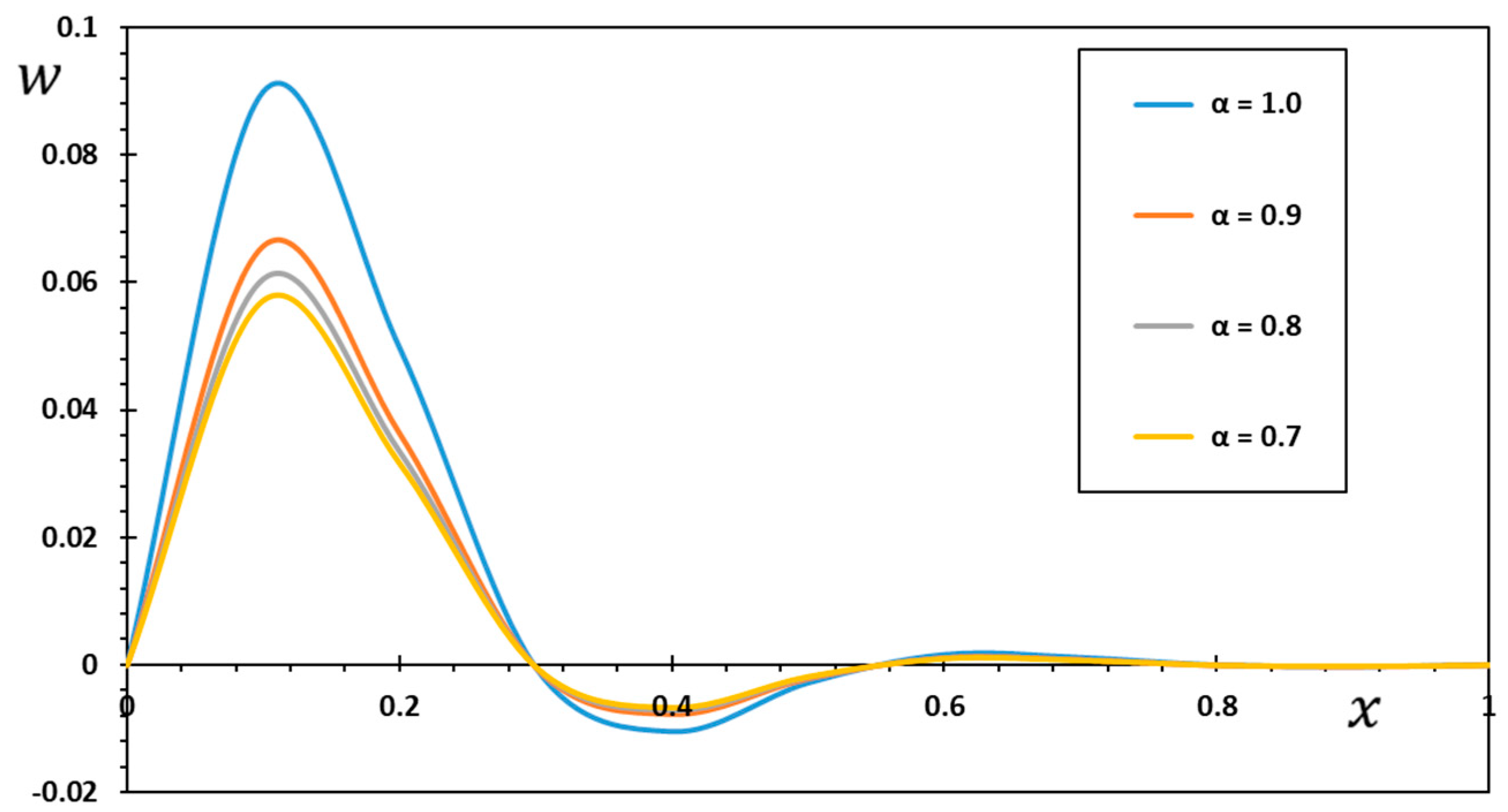
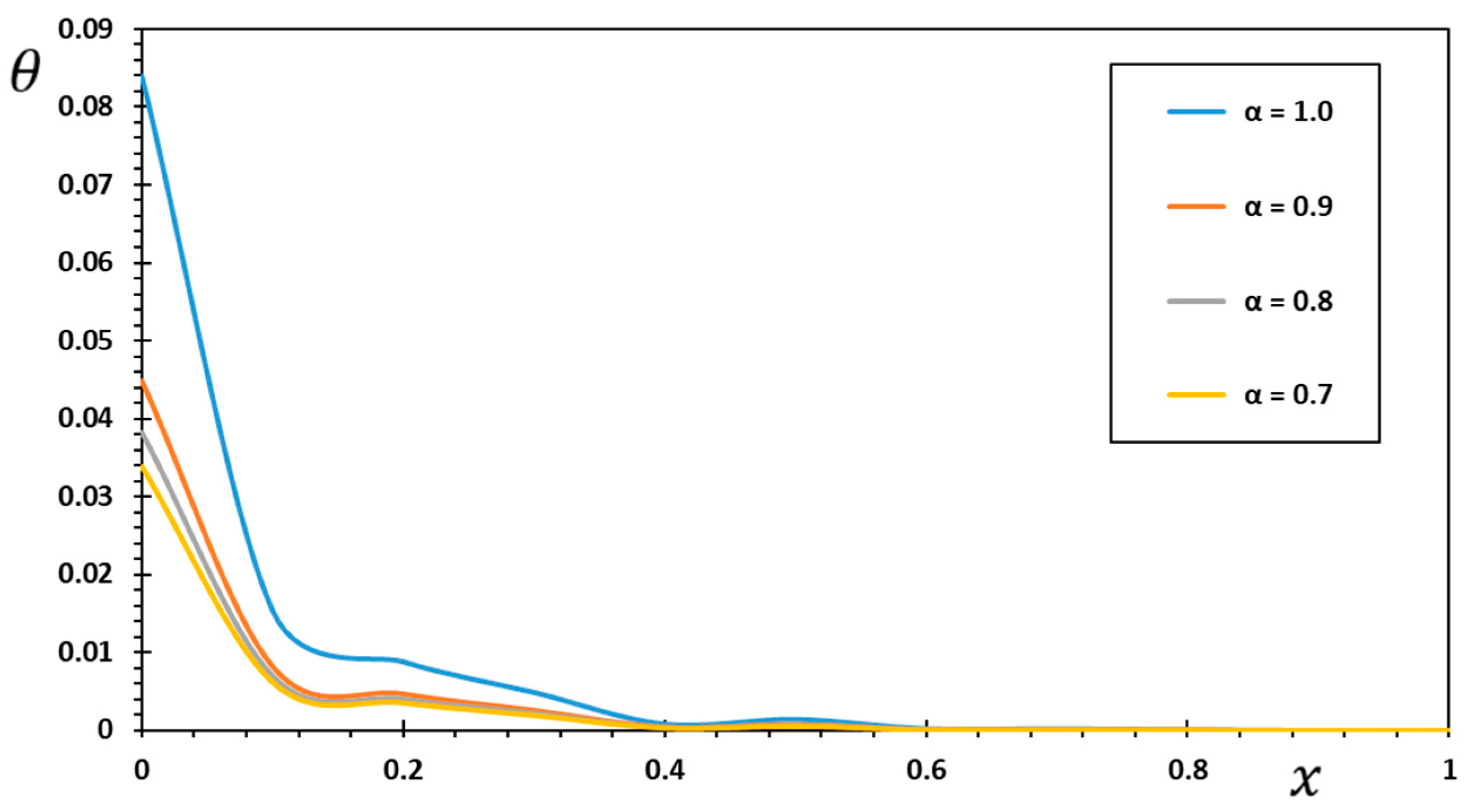
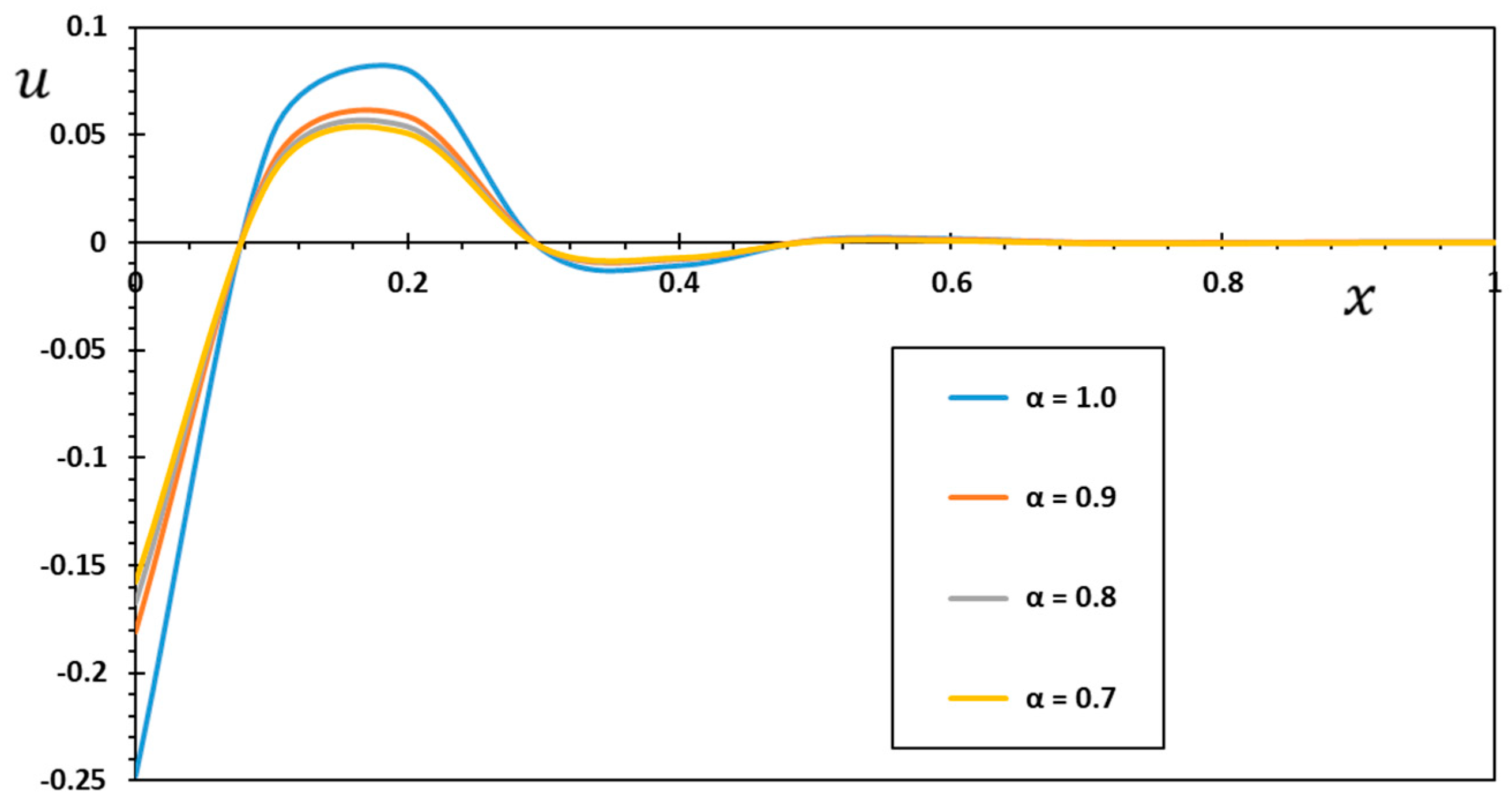
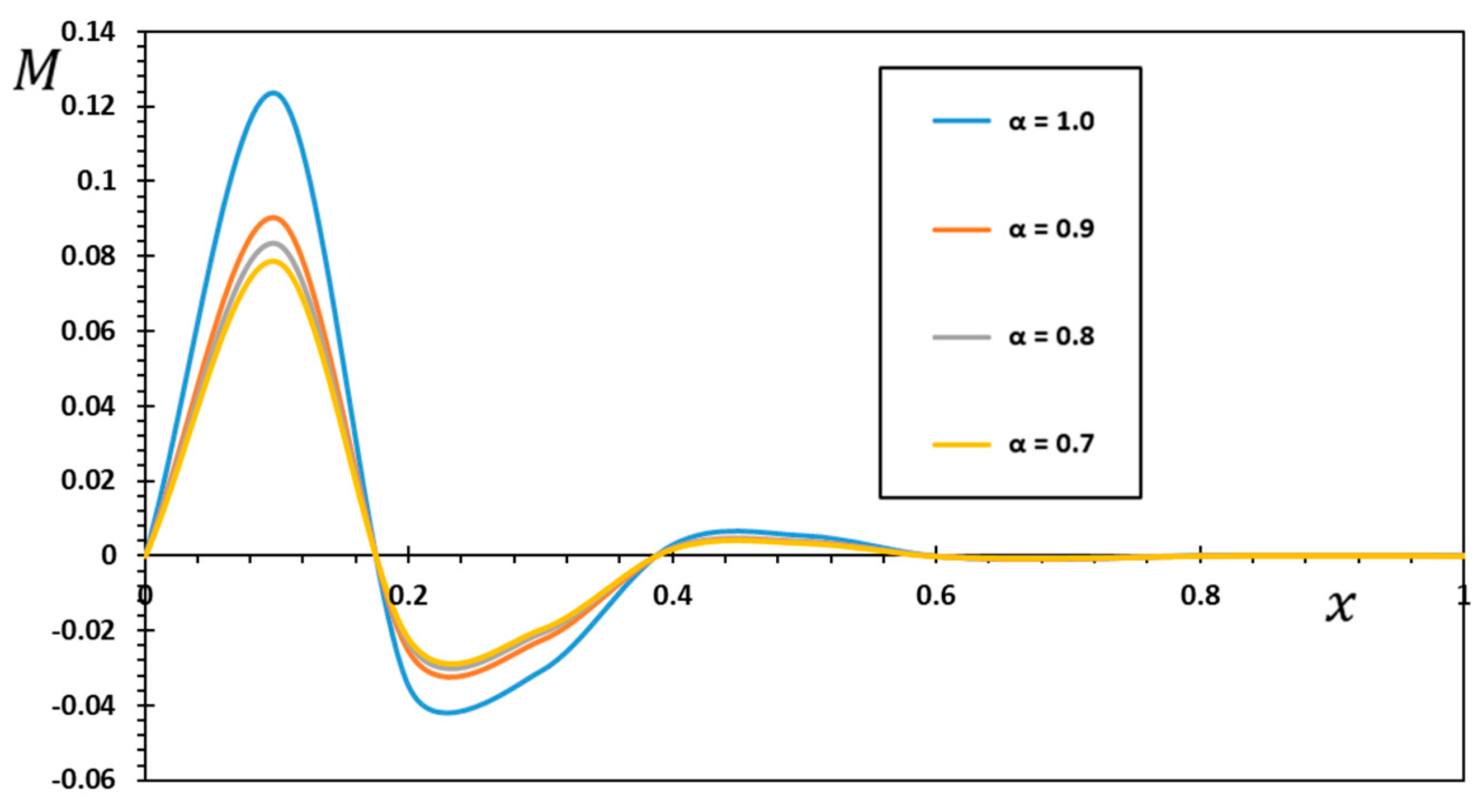
8.2. Impact of Fractional Derivative Parameter

In this work, we suggest an approximation to the solution of the fractional heat transfer equation defined by a non-singular fractional derivative. Our research employs the fractional derivative introduced by Atangana–Baleanu (AB) and Caputo. Fractional versions have a tremendous advantage over their conventional counterparts by having unlimited degrees of freedom for orders of derivatives and fully explaining the memory effect. To accomplish this, graphical illustrations have been developed to physically assess the consequences and compare the outcomes of the fractional derivatives for FGM nanoscale beams as compared to those of the classical approaches.

Due to the influence of fractional order, $\alpha$, in this subsection we will examine how the FG material reacts when subjected to a varying heat flux at regular intervals and how the reactions are distributed. The numerical solutions are computed for the situation when $\mathsf{\Omega }=3$, ${\tau }_0=0.02$, and $\xi =0.002$. The AB fractional derivative operator was used to graphically illustrate the temperature increment, $\theta$, the bending moment, $M$, the transverse vibration deviation, $w$, and the longitudinal displacement, $u$, in fractional thermoelastic for different fractional order values (see Figure 2, Figure 3, Figure 4 and Figure 5). When $\alpha =0.9, 0.8$, and $0.7$, the Atangana–Baleanu fractional derivative operator is utilized, and when $\alpha =1$, the classical nonfractional derivative is employed.

For various values of the fractional order parameter, $\alpha$, the relationship between the thermal deflection, $w$, and the distance, $x$, is shown in Figure 2. Figure 2 shows that the boundary requirements of the problem (48) are always satisfied by the zero values of the dispersed deflection, $w$, at the endpoints of the nanobeam. The nanobeam’s highest deflection occurs towards the first edge of the nanobeam due to the heat flow to which it is exposed, as opposed to other areas on the axial axis.

In Figure 3, we see how the fractional-order, $\alpha$, choices affect the temperature fluctuation, $\theta$, with distance, $x$, when subjected to an irregular thermal flow. Figure 3 demonstrates that as $x$ increases, the temperature, $\theta$, drops. Additionally, it is apparent from the nanobeam’s heat diffusion distribution curves that the most significant values of thermal diffusion are acquired near the beginning of the beam. The heat wave then weakens in its ability to reach the other side as $x$ is increased, and eventually, after a certain threshold has been passed, it vanishes altogether. In contrast to predictions based on traditional heat transfer models, the speed with which heat waves travel through the material is limited.

In comparison with the work of previous authors [67,68], these results are found to be compatible, and the conclusions are valid. In addition, this paper claims that theoretical models utilizing the Atangana–Baleanu fractional operator are superior at elucidating the true features of observed occurrences. To better explain complex situations in the real world, Atangana and Baleanu introduced the derivative using the Mittag–Leffler function. Thus, this new model of thermal conduction will definitely lead to understanding the new behavior of heat flow in nanobeams.

Figure 4 depicts the effect of the fractional-order parameter, $\alpha$, on a heterogeneous nanobeam to produce a range of displacement values, $u$, as a function of distance, $x$. We can see from the figure that the distortion, $u$, anisotropy increases as we move right on the beam axis. The magnitude of the displacement, $u$, gradually changes from positive to negative $x$ values. As the value of the fractional order parameter increases, the figure displays a more significant displacement away from the plane $x=0$. This is because the heat source experiences periodic and transient fluctuations. The axial displacement, $u$, of the nanobeam is reduced as the fractional parameters increase. Hence, it can be considered that the fractional derivative’s order affects the dynamics of thermal deformation in nanobeams at least in this present problem. By applying fractional-order derivatives in modeling techniques, a dynamic system aids in describing memory’s characteristics and efficacy (effectiveness, utility) as crucial elements in many nanostructured systems.

In Figure 5, we see how the fractional parameter affects the relationship between the thermal bending moment, $M$, and the distance, $x$. This image shows how the modulus can affect the bending moment of the nanobeam, $M$. It has also been shown that the peak bending moment grows under all conditions as the fractional parameter grows. The bending moments, $M$, calculated using the fractional derivative are offered as more minor in Figure 5 compared to those computed using the thermoelastic model with integer derivatives. The outcome of this investigation has shown that as the fractional order falls, the bending moment reduces. The fractional operator with the bending property developed by Atangana and Băleanu is responsible for this significant result.

The figures demonstrate how the rate at which waves travel can be affected by varying the value of the fractional-order parameter, $\alpha$. Therefore, it could be crucial to think about it while creating new materials for practical applications. In other words, when the values of the fractional order rise, it is possible to see the reduction of all curves in the different physical fields. This figure illustrates that when the current results are compared to those of [32], there is good agreement between the two data sets. As for the fractional case, it is noted that the different distributions in the case of using the fractional derivatives of AB are affected by the past more than the traditional derivative.

More practical recommendations are included in the current publication. It generally provides robust answers that converge rapidly on issues with an actual physical world component. The results can be helpful in cases where a perfect solution is not required and unnecessary complications must be avoided. However, it must be admitted that additional research on the topic may reveal hitherto unexplored possibilities, allowing for the development of more nuanced conclusions and extremely fruitful outcomes. As well as providing closed-form solutions to the specified issues, the detailed analysis has demonstrated the convergence of approximation results to precise answers. The convergence phenomena have proven that the suggested method is reliable. As a result, the fractional derivative of the Atangana–Baleanu in the Caputo concept can be used to describe fractional heat transfer equations.

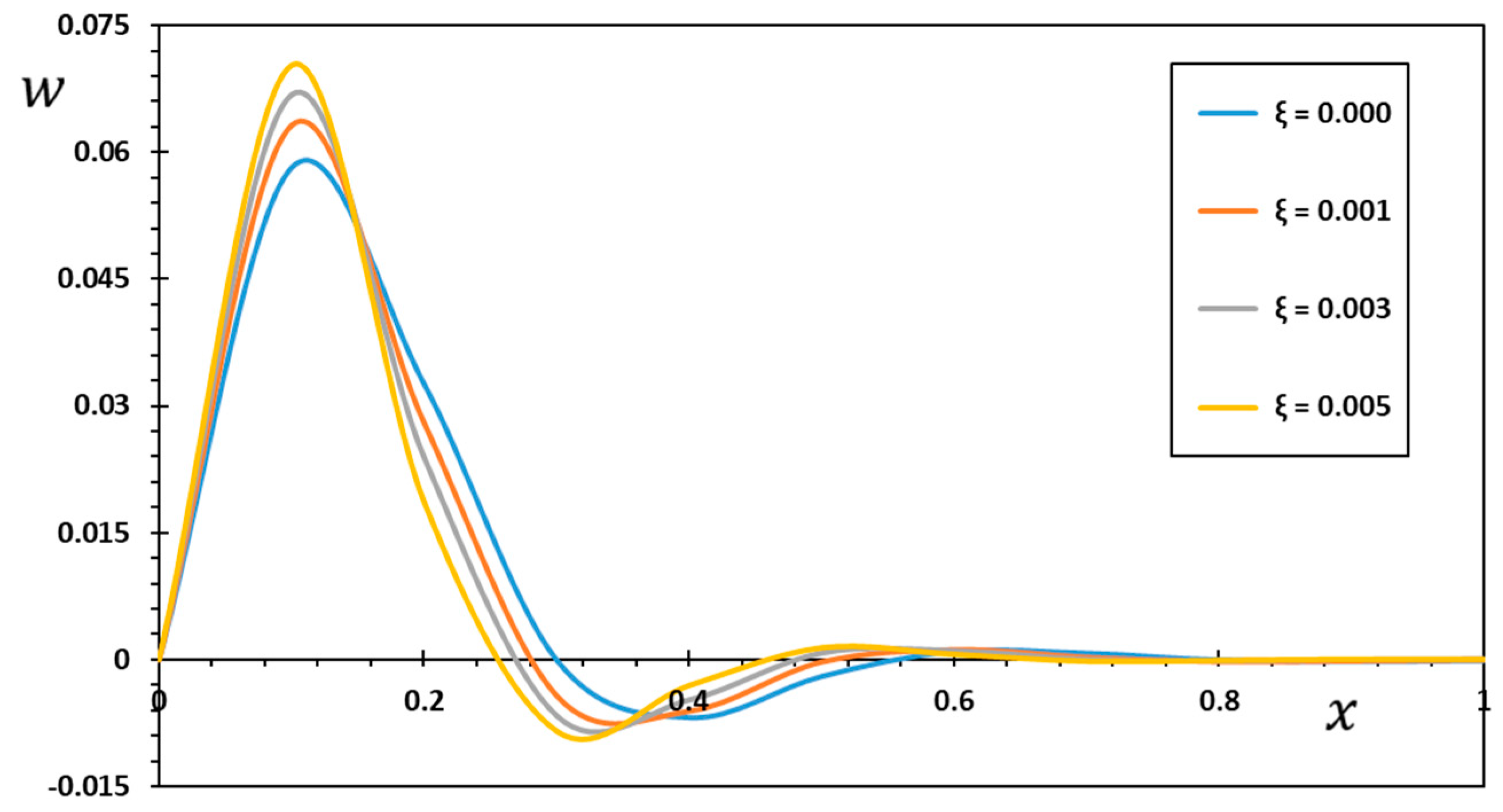
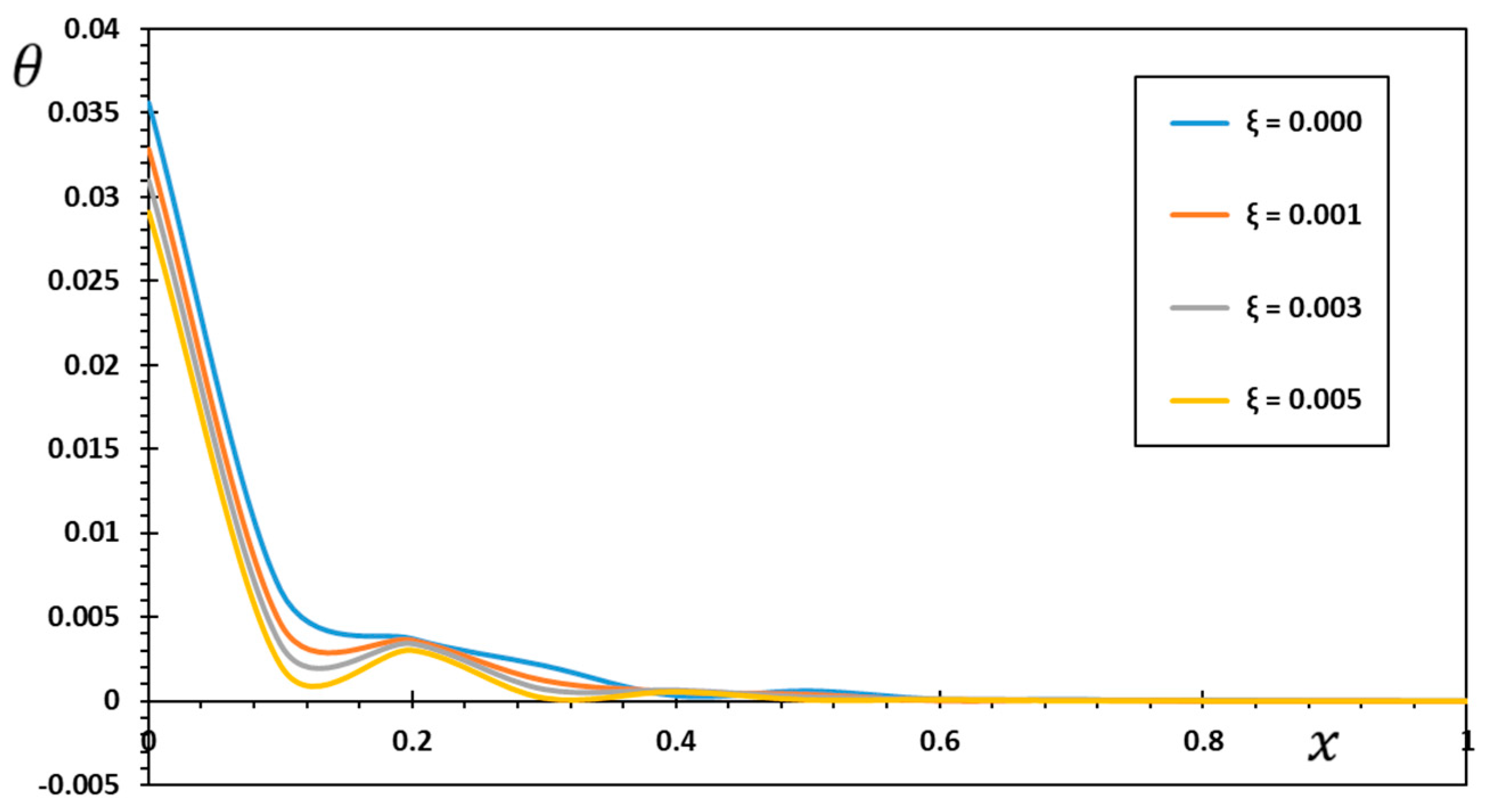
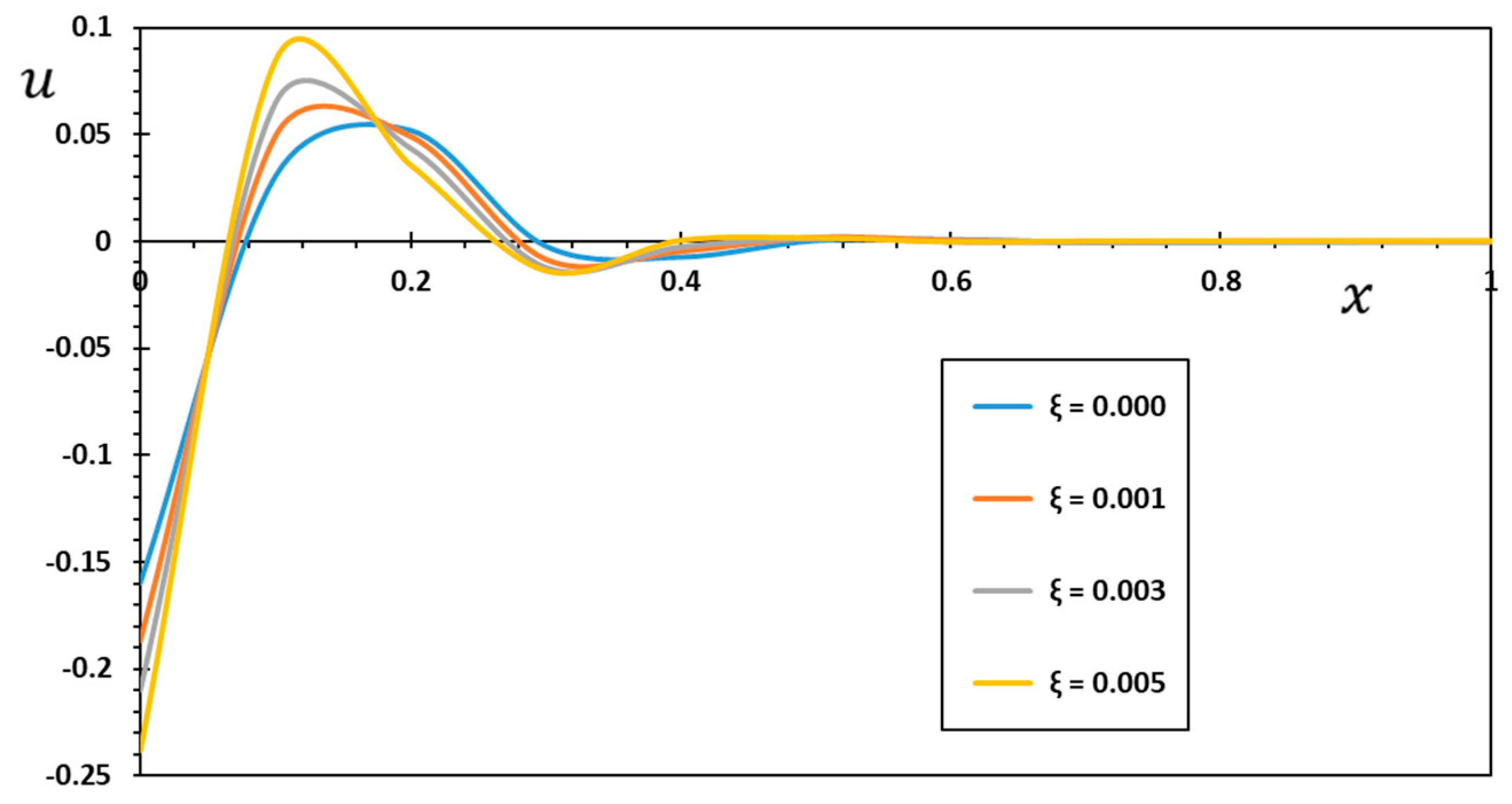
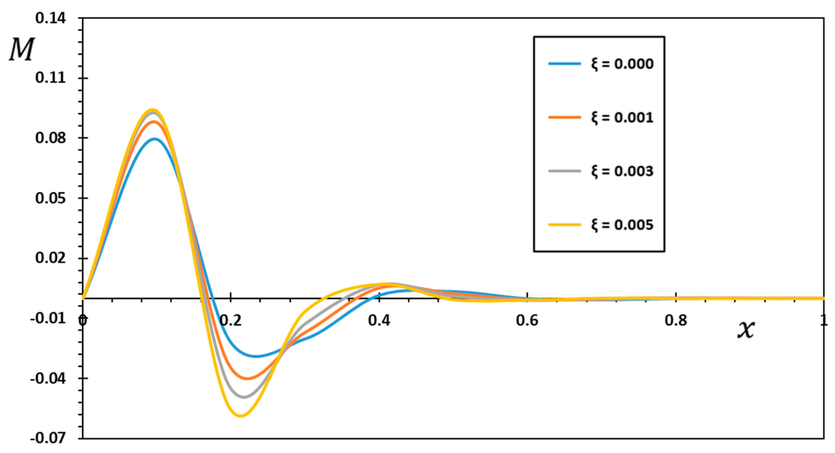
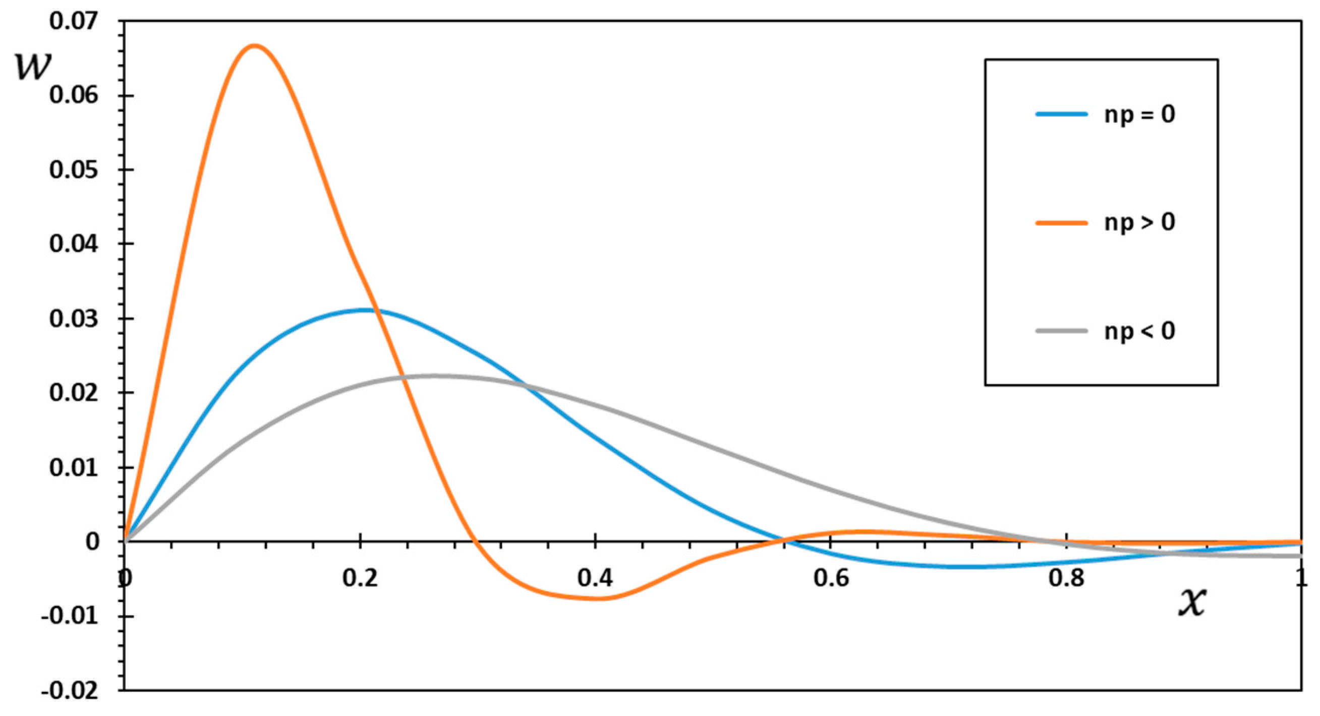
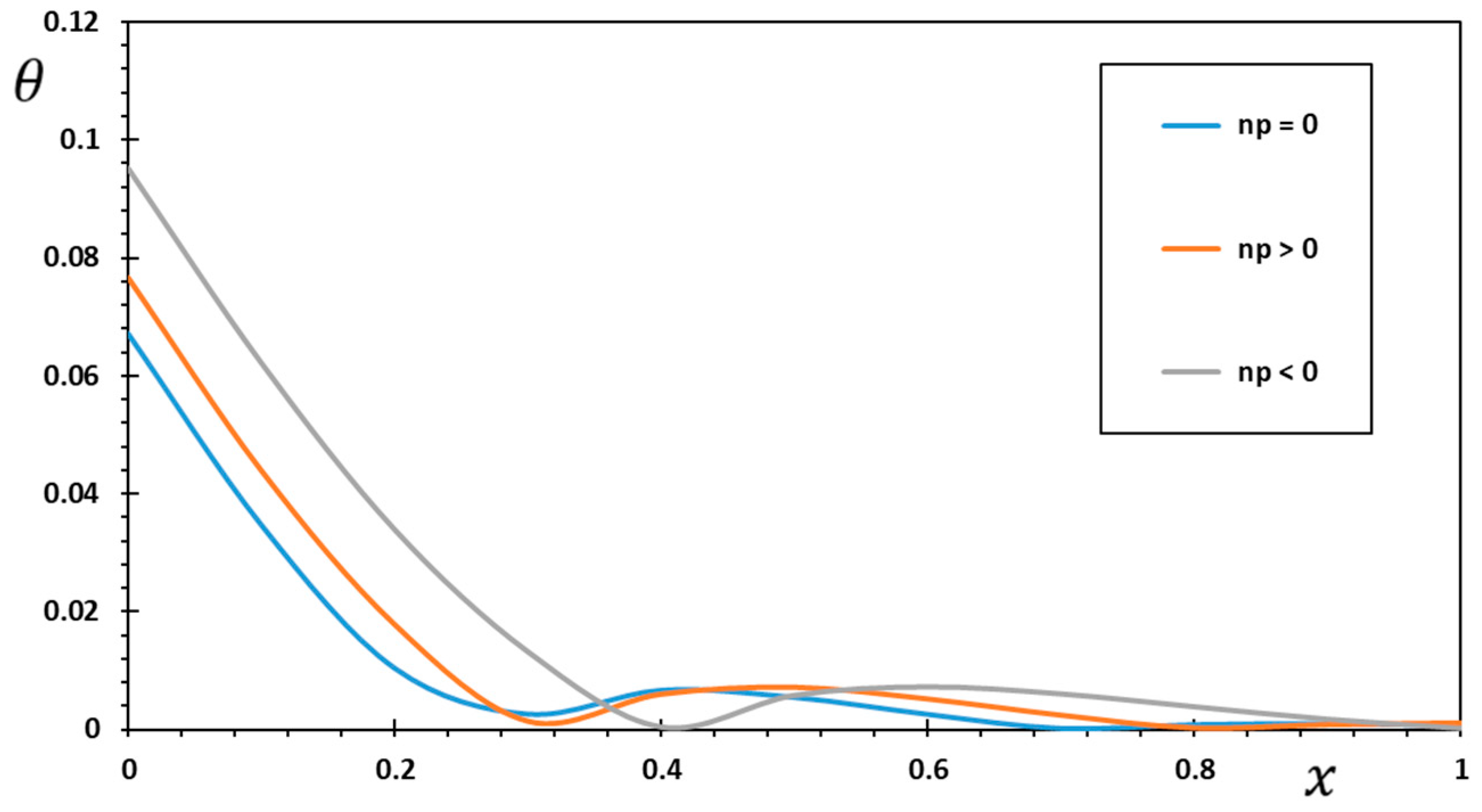
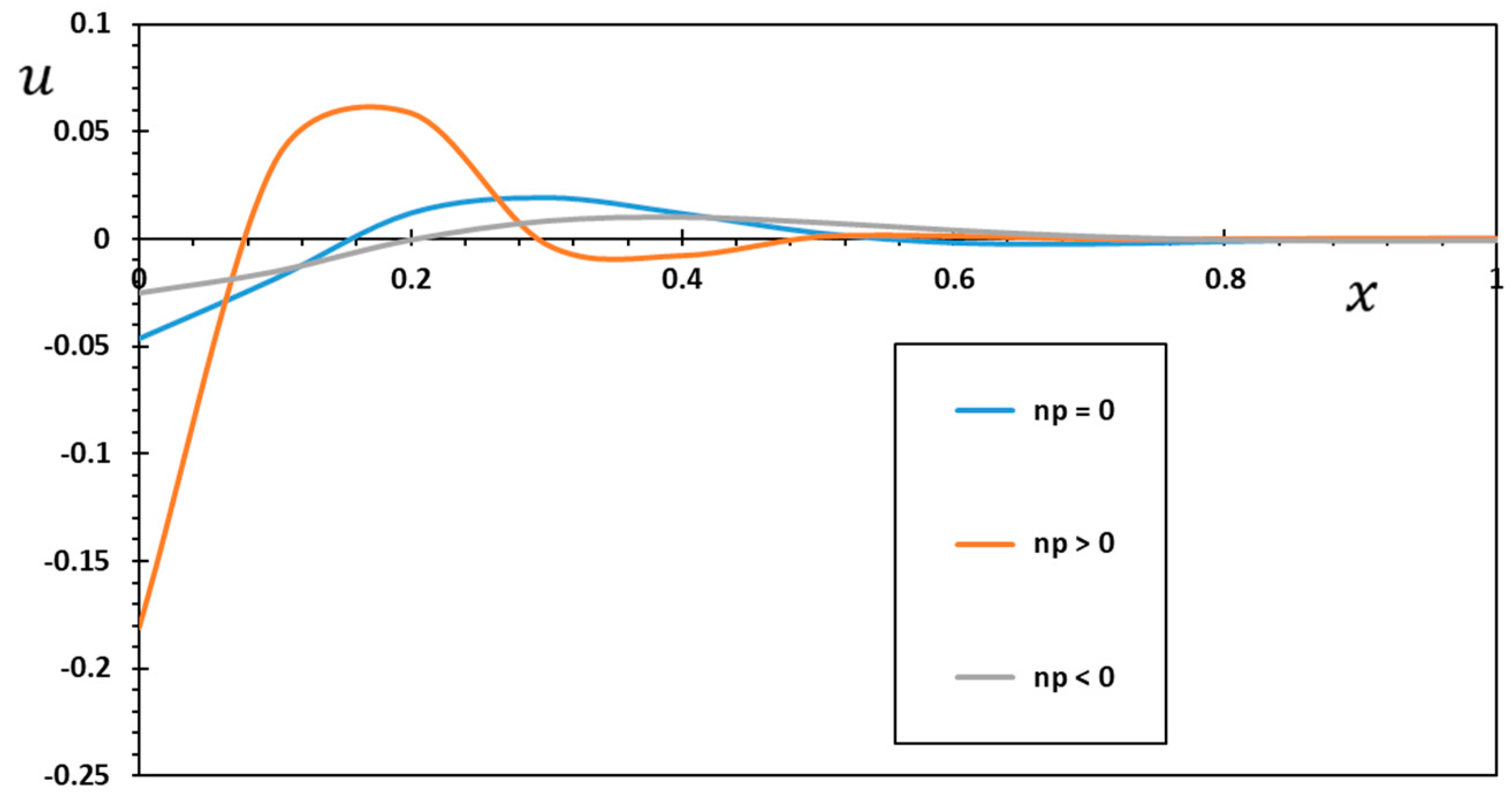
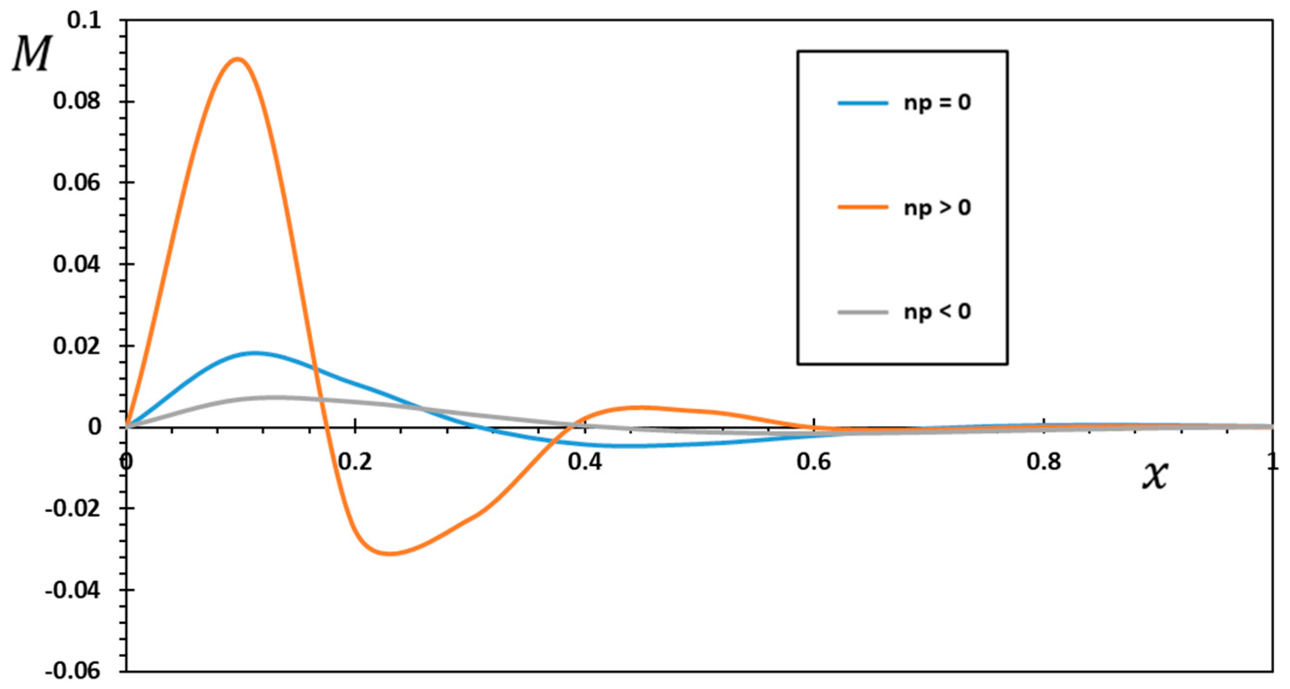
8.3. The Effect of Nonlocal Parameter

Nonlocal elasticity concepts have received much interest from researchers interested in designing or analyzing micro- or nanostructures. The models serve as models with bridging scales in the investigation of issues involving several scales because they extend the fundamental ideas in the classical theory of elasticity to approximate the behavior of particles as tiny as molecules or atoms. It is clear from the governing equations that these theories portray that they include one or more parameters in addition to the conventional constants. Because of these characteristics, also known as small-scale parameters, it is possible to investigate the size impact.

In contrast to earlier studies, the current study focuses on the extent to which nonlocal parameters affect the dynamic response of a functionally graded nanostructure in the context of physical and geometrical characteristics coupled with thermoelasticity theory involving differential operators of fractional orders. The nanostructure’s length is also considered because nonlocal events significantly affect how the nanostructure responds to vibrations. This study shows the variations in outcomes depending on conventional and non-conventional assumptions, in line with its intended purpose.

In this category, through Figure 6, Figure 7, Figure 8 and Figure 9, we have investigated how small-scale $\xi$ characteristics affect the fluctuations of several field variables ($w, \theta , u,$ and $M$). The remaining effective parameters ($\mathsf{\Omega }=3$, ${\tau }_0=0.02$, and $\alpha =0.8$) are assumed to remain unchanged in this case. When the value $\xi =0$ was present, the prior scenario (conventional beam theory) was suggested, but when $\xi =0.001$, $\xi =0.003$, and $\xi =0.005$ were present, the nonlocal elasticity theory (Eringen’s theory) was indicated. We show that the thermal deflection, temperature increment, bending moment, and axial displacement are very sensitive to the nonlocal parameter. The nonlocal parameter enhances the mechanical waves in all the fields examined. It can be explored that the influence of the nonlocal parameter on the axial changes of the nanobeam in different modes is prominent and, therefore, more significant. As shown in Figure 6, Figure 7, Figure 8 and Figure 9, as the value of the nonlocal parameter $\xi$ at given $x$ increases, the temperature curves decrease, and the amount of other physical fields increases. A softening impact was seen as the nonlocal parameter was increased. After the non-locality impact was introduced, the values of the major field variables under study decreased for both the mechanical and thermal systems.

In addition, it is clear from Figure 8 that throughout the axial direction of the beam, the axial displacement, $u$, increases with the nonlocal parameter at specific periods and decreases with it at others. Figure 6 shows that at $\xi =0.005$, the size of the deflection, $w$, is at its maximum. In Figure 9, it can be seen that the bending moment, $M$, profile grows in size when the nonlocal parameter values are raised. In addition, the displacement amount in the case of the local heat transfer model is less than the equivalent displacement curve for the nonlocal version (see Figure 8). As a result, to obtain trustworthy results, the nonlocal component of the motion equation must be taken into account, as it can change the results significantly. For this reason, future studies examining the mechanical behavior of micro- and nanostructures composed of FG materials may use the results of the proposed nonlocal theory as a valuable size-dependent framework. When the length-scale characteristics are considered, the curves demonstrate that we have a Stiffer nanosystem. So, considering nonclassical models will increase the system deflection and dynamic deformation. In addition, there are larger discrepancies between the nonlocal thermoelastic concept and traditional elasticity theory.

Researchers can use the results of this study to learn more about the instability of nanobeam-based tiny devices and make adjustments to their designs to boost their overall performance. As an added extra, this study’s results provide a rationale for why nonclassical frameworks, small-scale influences, and external dynamic and thermal force improvements to theoretical and experimental data provide different results when analyzing the reactions of the nano-system. Small-scale parameters are shown to be sensitive to the structure’s geometry, the qualities of the material it is made of, and the loads placed on it by means of the nonlocal interaction range factor. For this reason, ultra-small electronics based on nanostructures can only be modeled using nonlocal models.

8.4. The Effect of the Gradient Index

This subsection investigates the thermoelastic interaction of a functionally graded (FG) nanobeam using the nonlocal Euler–Bernoulli beam theory and the MGT heat transfer model. It is assumed that the FG nanobeam has material properties that change throughout its thickness. The length scale parameter (nonlocal parameter) is incorporated into this nonclassical (nonlocal) nanobeam framework to account for the small-scale effect.

It is investigated in Figure 10, Figure 11, Figure 12 and Figure 13 how the variability of the physically analyzed fields of the FG nanobeam is affected by the impact of the graded parameter $n_p$. Here, it is assumed that other parameters that often play a role remain unchanged ($\alpha =0.8,$ ${\tau }_0=0.02$ and $\xi =0.003$).

For three separate values of the graded parameter $n_p$, two values for the effective varying material properties ($n_p>0$ and $n_p<0$), and zero value $n_p=0$ for isotropic materials, the studied physical variables were calculated and investigated. The amplitudes of the nondimensional field variables examined are also shown to grow when the graded index $n_p>0$ (see Figure 10, Figure 11, Figure 12 and Figure 13). Once $n_p$ is specified, the nondimensional variables have their minimum values at $n_p=0$.

Increasing the gradient coefficient leads to an increase in the nondimensional deflections and a decrease in the dimensionless temperature. This is because the stiffness of the FG nanobeam increases as the gradient coefficient increases. When the gradient indicator is changed, there is a sudden shift in the responses, but once $n_p=0$ is reached, all the curves flatten out. In fact, FGMs are favored over conventional laminates because they offer uniformly smooth property variations throughout the whole surface, something that was not possible before when taking the interface between laminate plies into account [69]. In addition, while the individual plies of a composite laminate often behave in an anisotropic way, FGMs behave the same everywhere, even though they are made of different materials. The authors feel that the analyzed results will serve as a reference for other investigators to compare their findings because they are unaware of any previous work on the thermoelastic interactions in FG nanobeams.

9. Conclusions

This paper thoroughly studies a mathematical fractional thermoelastic framework for a functionally graded Euler–Bernoulli nanobeam subjected to a periodic heat flow. Variations in through-thickness features range from purely ceramic to purely metallic. The model employs both nonlocal elasticity theory and generalized MGT thermoelasticity with fractional derivative operators. The Atangana–Baleanu (AB) fractional derivative operator without singular kernels is a novel definition introduced by the revised heat conduction equation. Both analytical and numerical studies show that the nonhomogeneity parameter (gradient indicator), the nonlocal parameter, and the fractional differential operators significantly impact field variables. According to the results of the previous research:

• Thermomechanical responses of the FG nanobeam are shown to be significantly impacted by nonlocal effects, as demonstrated by numerical data.
• Magnitudes are bigger in the novel nonlocal beam model compared to the traditional (local) beam model. Therefore, the small-scale effects (also called nonlocal effects) must be considered when figuring out how nanostructures behave mechanically.
• The success of nonlocal beam models depends heavily on carefully selecting the nonlocal parameter’s value.
• The FG nanobeam’s responses can be adjusted by selecting appropriate values for the gradient indicator, which significantly impacts the responses.
• There were significant discrepancies between the variances of the thermoelastic models and the fractional thermoelastic models. Changes in the rate of change of the temperature variation depend strongly on the value of the fractional parameter of the Atangana–Baleanu fractional derivative operator. Therefore, the fractional parameter is becoming more effective as a measure of heat conduction.
• With fractional derivatives, the values of the fields under study are less than those predicted by standard thermoelastic models. Therefore, the fractional parameter should be chosen to reduce the medium’s effect on the elastic wave.
• Composite materials with FGM characteristics are superior to traditional homogenous materials in various contexts. The biomedical and defense industries also extensively use FGMs, most notably as medical implants and bulletproof vests. The automotive sector, the steel sector, the energy sector, etc., are just a few more areas where FGM has been found useful.
• With this new perspective on investigating thermal deformations in solid mechanics, we can understand the Atangana–Baleanu fractional derivative operator in heat and mass transfer systems. Application of the method and concepts given herein to other thermoelasticity and thermodynamic problems is possible.

References

1. Faghidian, S.A.; Żur, K.K.; Reddy, J.N.; Ferreira, A.J.M. On the wave dispersion in functionally graded porous Timoshenko-Ehrenfest nanobeams based on the higher-order nonlocal gradient elasticity. Compos. Struct. 2022, 279, 114819. [Google Scholar] [CrossRef]
2. Pham, Q.-H.; Tran, V.K.; Tran, T.T.; Nguyen, P.-C.; Malekzadeh, P. Dynamic instability of magnetically embedded functionally graded porous nanobeams using the strain gradient theory. Alex. Engin. J. 2022, 61, 10025–10044. [Google Scholar] [CrossRef]
3. Akgöz, B.; Civalek, Ö. Thermo-mechanical buckling behavior of functionally graded microbeams embedded in elastic medium. Int. J. Eng. Sci. 2014, 85, 90–104. [Google Scholar] [CrossRef]
4. Ghayesh, M.H.; Farokhi, H.; Amabili, M. Nonlinear behaviour of electrically actuated MEMS resonators. Int. J. Eng. Sci. 2013, 71, 137–155. [Google Scholar] [CrossRef]
5. Amiri Delouei, A.; Emamian, A.; Karimnejad, S.; Sajjadi, H. A closed-form solution for axisymmetric conduction in a finite functionally graded cylinder. Int. Communic. Heat Mass Trans. 2019, 108, 104280. [Google Scholar] [CrossRef]
6. Amiri Delouei, A.; Emamian, A.; Karimnejad, S.; Sajjadi, H.; Jing, D. Two-dimensional analytical solution for temperature distribution in FG hollow spheres: General thermal boundary conditions. Int. Communic. Heat Mass Trans. 2020, 113, 104531. [Google Scholar] [CrossRef]
7. Avey, M.; Fantuzzi, N.; Sofiyev, A. Mathematical modeling and analytical solution of thermoelastic stability problem of functionally graded nanocomposite cylinders within different theories. Mathematics 2022, 10, 1081. [Google Scholar] [CrossRef]
8. Kaur, I.; Singh, K.; Ghita, G.M.D.; Craciun, E.-M. Modeling of a magneto-electro-piezo-thermoelastic nanobeam with two temperature subjected to ramp type heating. Proc. Rom. Acad. Ser. A 2022, 23, 141–149. [Google Scholar]
9. Pinnola, F.P.; Barretta, R.; Marotti de Sciarra, F.; Pirrotta, A. Analytical solutions of viscoelastic nonlocal Timoshenko beams. Mathematics 2022, 10, 477. [Google Scholar] [CrossRef]
10. Wang, S.; Kang, W.; Yang, W.; Zhang, Z.; Li, Q.; Liu, M.; Wang, X. Hygrothermal effects on buckling behaviors of porous bi-directional functionally graded micro-/nanobeams using two-phase local/nonlocal strain gradient theory. Eur. J. Mech.-A/Solids 2022, 94, 104554. [Google Scholar] [CrossRef]
11. Civalek, Ö.; Uzun, B.; Yayl, M.Ö.; Akgöz, B. Size-dependent transverse and longitudinal vibrations of embedded carbon and silica carbide nanotubes by nonlocal finite element method. Eur. Phys. J. Plus 2020, 135, 381. [Google Scholar] [CrossRef]
12. Dangi, C.; Lal, R.; Sukavanam, N. Effect of surface stresses on the dynamic behavior of bi-directional functionally graded nonlocal strain gradient nanobeams via generalized differential quadrature rule. Eur. J. Mech.-A/Solids 2021, 90, 104376. [Google Scholar] [CrossRef]
13. Eringen, A.C. On differential equations of nonlocal elasticity and solutions of screw dislocation and surface waves. J. Appl. Phys. 1983, 54, 4703–4710. [Google Scholar] [CrossRef]
14. Eringen, A.C.; Edelen, D.G.B. On nonlocal elasticity. Int. J. Eng. Sci. 1972, 10, 233–248. [Google Scholar] [CrossRef]
15. Eringen, A.C. Linear theory of nonlocal elasticity and dispersion of plane waves. Int. J. Eng. Sci. 1972, 10, 425–435. [Google Scholar] [CrossRef]
16. Mindlin, R.D.; Eshel, N.N. On first strain-gradient theories in linear elasticity. Int. J. Solids Struct. 1968, 4, 109–124. [Google Scholar] [CrossRef]
17. Askes, H.; Aifantis, E.C. Gradient elasticity in statics and dynamics: An overview of formulations, length scale identification procedures, finite element implementations and new results. Int. J. Solids Struct. 2011, 48, 1962–1990. [Google Scholar] [CrossRef]
18. Lam, D.C.C.; Yang, F.; Chong, A.C.M.; Wang, J.; Tonga, P. Experiments and theory in strain gradient elasticity. J. Mech. Phys. Solids 2003, 51, 1477–1508. [Google Scholar] [CrossRef]
19. Grekova, E.F.; Porubov, A.V.; dell’Isola, F. Reduced linear constrained elastic and viscoelastic homogeneous Cosserat media as acoustic metamaterials. Symmetry 2020, 12, 521. [Google Scholar] [CrossRef] [Green Version]
20. Toupin, R.A. Elastic materials with couple-stresses. Arch. Ration Mech. Anal. 1962, 11, 385–414. [Google Scholar] [CrossRef] [Green Version]
21. Toupin, R.A. Theories of elasticity with couple-stress. Arch. Ration Mech. Anal. 1964, 17, 85–112. [Google Scholar] [CrossRef]
22. Atangana, A.; Secer, A. A note on fractional order derivatives and table of fractional derivatives of some special functions. Abst. Appl. Analy. 2013, 2013, 279681. [Google Scholar] [CrossRef] [Green Version]
23. Patnaik, S.; Hollkamp, J.P.; Semperlotti, F. Applications of variable-order fractional operators: A review. Proc. R. Soc. A Math. Phys. Eng. Sci. 2020, 476, 20190498. [Google Scholar] [CrossRef] [PubMed] [Green Version]
24. Caputo, M.; Fabrizio, M. A new definition of fractional derivative without singular kernel. Prog. Fract. Differ. Appl. 2015, 1, 73–85. [Google Scholar]
25. Atangana, A.; Baleanu, D. New fractional derivative with nonlocal and nonsingular kernel. Therm. Sci. 2016, 20, 757. [Google Scholar] [CrossRef] [Green Version]
26. Atangana, A.; Baleanu, D. New fractional derivatives with nonlocal and non-singular kernel: Theory and application to heat transfer model. Therm. Sci. 2016, 20, 763–769. [Google Scholar] [CrossRef] [Green Version]
27. Saad, K.M. New fractional derivative with non-singular kernel for deriving Legendre spectral collocation method, Alex. Eng. J. 2020, 59, 1909–1917. [Google Scholar]
28. Dokuyucu, M.A.; Dutta, H.; Yildirim, C. Application of nonlocal and non-singular kernel to an epidemiological model with fractional order. Math. Methods Appl. Sci. 2021, 44, 3468–3484. [Google Scholar] [CrossRef]
29. Sabatier, J. Non-Singular kernels for modelling power law type long memory behaviours and beyond. Cybern. Sys. 2020, 51, 383–401. [Google Scholar] [CrossRef]
30. Aljahdaly, N.H.; Agarwal, R.P.; Shah, R.; Botmart, T. Analysis of the time fractional-order coupled burgers equations with non-singular kernel operators. Mathematics 2021, 9, 2326. [Google Scholar] [CrossRef]
31. Anastassiou, G.A. Multiparameter fractional differentiation with non singular kernel. Probl. Anal.-Iss. Analy. 2021, 10, 15–30. [Google Scholar] [CrossRef]
32. Heydari, M.H.; Hosseininia, M. A new variable-order fractional derivative with non-singular Mittag–Leffler kernel: Application to variable-order fractional version of the 2D Richard equation. Engin. Comput. 2022, 38, 1759. [Google Scholar] [CrossRef]
33. Jena, R.M.; Chakraverty, S. Singular and Nonsingular Kernels Aspect of Time-Fractional Coupled Spring-Mass System. ASME J. Comput. Nonlinear Dynam. 2022, 17, 021001. [Google Scholar] [CrossRef]
34. Atangana, A.; Akgül, A.; Owolabi, K.M. Analysis of fractal fractional differential equations. Alex. Eng. J. 2020, 59, 1117–1134. [Google Scholar] [CrossRef]
35. Atangana, A.; Qureshi, S. Modeling attractors of chaotic dynamical systems with fractal-fractional operators. Chaos Solitons Fractals 2019, 123, 320–337. [Google Scholar] [CrossRef]
36. Saad, K.M.; Gómez-Aguilar, J.F. Analysis of reaction–diffusion system via a new fractional derivative with non-singular kernel. Phys. A Stat. Mech. Its Appl. 2018, 509, 703–716. [Google Scholar] [CrossRef]
37. Fernandez, A.; Baleanu, D. Classes of operators in fractional calculus: A case study. Math. Methods Appl. Sci. 2021, 44, 9143–9162. [Google Scholar] [CrossRef]
38. Lord, H.W.; Shulman, Y. A generalized dynamical theory of thermoelasticity. J. Mech. Phys. Solids 1967, 15, 299–309. [Google Scholar] [CrossRef]
39. Green, A.E.; Naghdi, P.M. Thermoelasticity without energy dissipation. J. Elast. 1993, 31, 189–208. [Google Scholar] [CrossRef]
40. Green, A.E.; Naghdi, P.M. On undamped heat waves in an elastic solid. J. Therm. Stress. 1992, 15, 253–264. [Google Scholar] [CrossRef]
41. Green, A.E.; Naghdi, P.M. A re-examination of the basic postulates of thermomechanics. Proc. R. Soc. Lond. A. 1991, 432, 171–194. [Google Scholar]
42. Quintanilla, R. Moore–Gibson–Thompson thermoelasticity. Math. Mech. Solids 2019, 24, 4020–4031. [Google Scholar] [CrossRef]
43. Quintanilla, R. Moore-Gibson-Thompson thermoelasticity with two temperatures. Appl. Eng. Sci. 2020, 1, 100006. [Google Scholar] [CrossRef]
44. Moaaz, O.; Abouelregal, A.E.; Alsharari, F. Analysis of a transversely isotropic annular circular cylinder immersed in a magnetic field using the Moore–Gibson–Thompson thermoelastic model and generalized Ohm’s law. Mathematics 2022, 10, 3816. [Google Scholar] [CrossRef]
45. Abouelregal, A.E.; Dassios, I.; Moaaz, O. Moore–Gibson–Thompson Thermoelastic Model Effect of Laser-Induced Microstructures of a Microbeam Sitting on Visco-Pasternak Foundations. Appl. Sci. 2022, 12, 9206. [Google Scholar] [CrossRef]
46. Abouelregal, A.E.; Mohammed, F.A.; Benhamed, M.; Zakria, A.; Ahmed, I.-E. Vibrations of axially excited rotating micro-beams heated by a high-intensity laser in light of a thermo-elastic model including the memory-dependent derivative. Math. Comp. Simul. 2022, 199, 81–99. [Google Scholar] [CrossRef]
47. Moaaz, O.; Abouelregal, A.E.; Alesemi, M. Moore–Gibson–Thompson Photothermal Model with a Proportional Caputo Fractional Derivative for a Rotating Magneto-Thermoelastic Semiconducting Material. Mathematics 2022, 10, 3087. [Google Scholar] [CrossRef]
48. Abouelregal, A.E. Generalized thermoelastic MGT model for a functionally graded heterogeneous unbounded medium containing a spherical hole. Eur. Phys. J. Plus 2022, 137, 953. [Google Scholar] [CrossRef]
49. Abouelregal, A.E.; Mohammad-Sedighi, H.; Shirazi, A.H.; Malikan, M.; Eremeyev, V.A. Computational analysis of an infinite magneto-thermoelastic solid periodically dispersed with varying heat flow based on nonlocal Moore–Gibson–Thompson approach. Contin. Mech. Thermodyn. 2022, 34, 1067–1085. [Google Scholar] [CrossRef]
50. Abouelregal, A.E.; Moustapha, M.V.; Nofal, T.A.; Rashid, S.; Ahmad, H. Generalized thermoelasticity based on higher-order memory-dependent derivative with time delay. Results Phys. 2021, 20, 103705. [Google Scholar] [CrossRef]
51. Eringen, A.C.; Wegner, J. Nonlocal Continuum Field Theories. ASME Appl. Mech. Rev. March. 2003, 56, B20–B22. [Google Scholar] [CrossRef]
52. Miller, K.S.; Ross, B. An introduction to the Fractional Integrals and Derivatives, Theory and Applications; John Wiley and Sons Inc.: New York, NY, USA, 1993. [Google Scholar]
53. Atangana, A.; Baleanu, D. Caputo-Fabrizio derivative applied to groundwater flow within confined aquifer. J. Eng. Mech. 2017, 143, D4016005. [Google Scholar] [CrossRef]
54. Zhang, N.; Khan, T.; Guo, H.; Shi, S.; Zhong, W.; Zhang, W. Functionally graded materials: An overview of stability, buckling, and free vibration analysis. Advan. Mater. Sci. Eng. 2019, 2019, 1354150. [Google Scholar] [CrossRef] [Green Version]
55. Gupta, A.; Talha, M. Recent development in modeling and analysis of functionally graded materials and structures. Prog. Aero. Sci. 2015, 79, 1–14. [Google Scholar] [CrossRef]
56. Abouelregal, A.E.; Mohammed, W.W.; Mohammad-Sedighi, H. Vibration analysis of functionally graded microbeam under initial stress via a generalized thermoelastic model with dual-phase lags. Arch. Appl. Mech. 2021, 91, 2127–2142. [Google Scholar] [CrossRef]
57. Abouelregal, A.E.; Ahmad, H.; Yao, S.-W. Functionally graded piezoelectric medium exposed to a movable heat flow based on a heat equation with a memory-dependent derivative. Materials 2020, 13, 3953. [Google Scholar] [CrossRef] [PubMed]
58. Oden, J.T.; Ripperger, E.A. Mechanics of Elastic Structures; Hemisphere/McGraw-Hill: New York, NY, USA, 1981. [Google Scholar]
59. Peng, W.; Chen, L.; He, T. Nonlocal thermoelastic analysis of a functionally graded material microbeam. Appl. Math. Mech.-Engl. Ed. 2021, 42, 855. [Google Scholar] [CrossRef]
60. Honig, G.; Hirdes, U. A method for the numerical inversion of the Laplace transform. J. Comp. Appl. Math. 1984, 10, 113–132. [Google Scholar] [CrossRef] [Green Version]
61. Abbas, I.; Hobiny, A.; Alshehri, H.; Vlase, S.; Marin, M. Analysis of Thermoelastic Interaction in a Polymeric Orthotropic Medium Using the Finite Element Method. Polymers 2022, 14, 2112. [Google Scholar] [CrossRef]
62. Abbas, I.; Marin, M.; Hobiny, A.; Vlase, S. Thermal Conductivity Study of an Orthotropic Medium Containing a Cylindrical Cavity. Symmetry 2022, 14, 2387. [Google Scholar] [CrossRef]
63. Hobiny, A.; Abbas, I. Generalized Thermo-Diffusion Interaction in an Elastic Medium under Temperature Dependent Diffusivity and Thermal Conductivity. Mathematics 2022, 10, 2773. [Google Scholar] [CrossRef]
64. Abouelregal, A.E.; Marin, M. The size-dependent thermoelastic vibrations of nanobeams subjected to harmonic excitation and rectified sine wave heating. Mathematics 2020, 8, 1128. [Google Scholar] [CrossRef]
65. Abouelregal, A.E.; Marin, M. The response of nanobeams with temperature-dependent properties using state-space method via modified couple stress theory. Symmetry 2020, 12, 1276. [Google Scholar] [CrossRef]
66. Kaur, I.; Singh, K. Functionally graded nonlocal thermoelastic nanobeam with memory-dependent derivatives. SN Appl. Sci. 2022, 4, 329. [Google Scholar] [CrossRef]
67. Sene, N. Fractional diffusion equation described by the Atangana-Baleanu fractional derivative and its approximate solution. J. Frac. Calc. Nonlinear Sys. 2021, 2, 60–75. [Google Scholar] [CrossRef]
68. Mittal, G.; Kulkarni, V.S. Two temperature fractional order thermoelasticity theory in a spherical domain. J. Therm. Stress. 2019, 42, 1136–1152. [Google Scholar] [CrossRef]
69. Abouelregal, A.E. Mathematical modeling of functionally graded nanobeams via fractional heat Conduction model with non-singular kernels. Arch. Appl. Mech. 2022. [Google Scholar] [CrossRef]
Figure 1. Configuration of FG thermoelastic nanobeam.
Mathematics 10 04718 g001
Figure 2. Effect of fractional order, α , on the deflection, w .
Mathematics 10 04718 g002
Figure 3. Effect of fractional order, α , on the temperature, θ .
Mathematics 10 04718 g003
Figure 4. Effect of fractional order, α , on the displacement, u .
Mathematics 10 04718 g004
Figure 5. Effect of fractional order, α , on the bending moment, M .
Mathematics 10 04718 g005
Figure 6. The thermal deflection, w , under various nonlocal parameter ξ values.
Mathematics 10 04718 g006
Figure 7. The dimensionless temperature, θ , under various nonlocal parameter ξ values.
Mathematics 10 04718 g007
Figure 8. The axial displacement, u , under various nonlocal parameter ξ values.
Mathematics 10 04718 g008
Figure 9. The bending moment, M , under various nonlocal parameter ξ values.
Mathematics 10 04718 g009
Figure 10. Effect of the gradient indicator on the dimensionless deflection, w .
Mathematics 10 04718 g010
Figure 11. Effect of the gradient indicator on the dimensionless temperature, θ .
Mathematics 10 04718 g011
Figure 12. Effect of the gradient indicator on the dimensionless displacement, u .
Mathematics 10 04718 g012
Figure 13. Effect of the gradient indicator on the dimensionless bending moment, M .
Mathematics 10 04718 g013