Article

A Branch-and-Bound Algorithm for the Bi-Objective Quay Crane Scheduling Problem Based on Efficiency and Energy

1
College of Management and Economics, Tianjin University, Tianjin 300072, China
2
Zhou Enlai School of Government, Nankai University, Tianjin 300350, China
3
Chinese Government and Policy Joint Research Center, Nankai University, Tianjin 300350, China
*
Author to whom correspondence should be addressed.
Mathematics 2022, 10(24), 4705; https://doi.org/10.3390/math10244705
Submission received: 24 October 2022 / Revised: 29 November 2022 / Accepted: 8 December 2022 / Published: 11 December 2022

Abstract

:
Motivated by the call of the International Maritime Organization to meet the emission targets of 2030, this study considers two important practical aspects of quay crane scheduling: efficiency and energy consumption. More precisely, we introduce the bi-objective quay crane scheduling problem where the objective is to minimize the vessel’s completion time and the crane’s energy consumption. This is done by formulating a bi-objective mixed-integer programming model. A branch-and-bound algorithm was developed as the exact solution approach to find the full set of Pareto-optimal solutions. We consider (i) various lower bounds for both objectives, (ii) specific upper bounds, (iii) additional branching criteria, and (iv) fathoming criteria to detect Pareto-optimal solutions. Numerical experiments on benchmark instances show that the branch-and-bound algorithm can efficiently solve small- and medium-sized problems.

1. Introduction

Container ports, as key players in international trade and logistics, continue to underpin global supply chain operations. In 2021, world container ports throughput stood at 897 million TEUs (twenty-foot equivalent units), reflecting an additional 10.1% as the global economy and trade recover [1]. Hence, the topic of operations management for container terminals has attracted considerable interest. Among them, various scheduling decisions play important roles in seaside operations, which typically include cranes [2], vehicles [3], and manpower [4].
The general scheduling problem consists of the assignment of tasks to equipment and the temporal arrangement of the tasks subject to precedence relationships and sequence-dependent setup times [5]. Most studies of single-objective scheduling problems result in a schedule to minimize the time required to complete all tasks (i.e., makespan). For the decision-maker in container terminals; however, this type of problem often consists of finding trade-offs between, e.g., time and energy consumption. Therefore, the single-objective problem needs to be extended to a multi-objective version.
With the Paris Agreement on global climate change in 2015, and the publishing of the UN Sustainable Development Goals (SDGs) in the same year, it is only natural that container ports are increasingly becoming involved in sustainable practices and how they can adopt these to align with the SDGs. According to the estimates of the International Maritime Organization (IMO), greenhouse gas (GHG) emissions from international shipping accounts for 2.2% of anthropogenic carbon dioxide emissions, and its share could increase to between 50% and 250% by 2050 [6].
Container handling operations, especially crane operations, have significant impacts on global GHG emissions. It is estimated that electricity contributes to approximately 18% of total GHG emissions at the Barcelona port [7]. Among them, a significant share of GHG emissions from electricity is derived from cranes. In the Port of Los Angeles, for example, the total GHG emissions of quay cranes for cargo handling is 1594.5 tons, accounting for 48.03% of the GHG emissions of equipment during cargo handling [8]. Thus, reducing GHG emissions by saving energy during the loading and unloading of cranes is critical for port operations, management, planning, as well as for meeting globally established sustainability benchmarks and objectives.
In this paper, we study the quay crane scheduling problem with energy consumption (QCSPEC) to balance time-savings and energy-savings (and, thereby, emission-reducing). We formulate a bi-objective mixed integer programming model with the objective of minimizing the vessel completion time and the total handling energy consumption of cranes. Due to the difficulty in solving the mathematical formulation using the solver (e.g., CPLEX, GUROBI, and X-PRESS MP), we developed a branch-and-bound algorithm to find the full set of Pareto-optimal solutions. Numerical experiments were conducted to validate the effectiveness of the proposed model and solution method. To the best of our knowledge, our work is the first in the literature to provide a systematic approach for identifying the Pareto-optimal front for the bi-objective quay crane scheduling problem by an exact method.

2. Literature Review

In this section, we first review the relevant literature on QCSP. In particular, we restrict ourselves to the unidirectional QCSP, which requires that all cranes move in the same direction, from bow to stern or vice versa. After that, we present studies that focused on energy savings and emission reductions of container terminals. We then review the literature related to the Pareto-optimization approach. Finally, we conclude our contribution.

2.1. Quay Crane Scheduling at Container Terminals

The QCSP has been researched for more than 30 years, as first introduced by Daganzo [9]. Subsequently, many scholars conducted extensive research on the QCSP. Comprehensive overviews on applications and optimization models in this field are given by Bierwirth and Meisel [10,11]. In this paper, we research a special counterpart of QCSP known as unidirectional QCSP, which requires that all cranes move along the bow to the stern or in the opposite direction throughout the working period after initial repositioning. The unidirectional QCSP was first incorporated by Liu et al. [12]; the authors developed a two-level framework that covers a wide variety of problem constraints. They formulated a mixed integer linear programming (MILP) model for unidirectional QCSP at the vessel level that finds the minimum completion time of a vessel for a given number of cranes assigned to it. Bierwirth and Meisel [13] designed a branch-and-bound heuristic algorithm to solve the unidirectional QCSP with interference constraints. The basic idea of the proposed heuristic is to exhaustively search for the space of unidirectional schedules, and finally obtain the optimal solution among the unidirectional ones. Based on this study, Meisel [14] further studied the unidirectional QCSP with time windows; the author proposed a new problem-oriented algorithm that limits the search to the unidirectional ones. Later, Legato et al. [15] formulated a MILP model for the unidirectional QCSP, which considered the non-uniform service rate of cranes. They extended the algorithm proposed by Bierwirth and Meisel [13] to find optimal unidirectional schedules in a shorter time. Legato and Trunfio [16] developed a precise framework for solving unidirectional QCSP, which incorporates the local branching method into a branch-and-bound algorithm. This method further improves the method proposed by Bierwirth and Meisel [13] and Legato et al. [15] and shows a higher solution performance. Chen et al. [17] considered the blocking phenomena in the initial stage of the scheduling and proposed an enhanced unidirectional QCSP model that reinforces the MILP model proposed by Liu et al. [12], and the strengthened model can be easily solved by a standard optimization solver. Further, Chen and Bierlaire [18] analyzed the computational complexity of the unidirectional QCSP and showed that the unidirectional QCSP is NP-hard. Recently, Ma et al. [19] further extended the deterministic unidirectional QCSP to a stochastic version. Overall, most of the existing research studies are focused on improving the throughput of terminals and shortening ship turnaround times by lifting loading and unloading efficiency. Nevertheless, energy saving and emission reduction at container terminals also need to be considered.

2.2. Energy Saving and Emission Reduction at Container Terminals

For energy saving or emission reduction of container terminals, most studies focus on the fuel consumption or emissions from vessels sailing or berthing (see, for instance, [20,21]). For a comprehensive overview of energy saving and emission reduction for vessels, we refer the reader to Psaraftis and Kontovas [22]. In addition, energy consumption or emissions on container terminal operations are mainly concentrated at the macro level, such as policies, planning, and environmental impact assessment. For further details, we refer the reader to the review work given by Mansouri et al. [23]. A few studies have focused on energy-saving or GHG emissions from port operations. In the scarce literature on energy saving or emission reduction at the operational level, Chang et al. [24] proposed an integrated model for berth allocation and quay crane assignments, which simultaneously optimize three objectives, including the energy consumption of cranes. However, when solving, three non-comparable objectives were scalarized to a single objective that can then be easily evaluated. Esmemr et al. [25] used a simulation model to determine the optimum number of container handling equipment to reduce damage to the environment of the Turkish port. Chen et al. [26] proposed a bi-objective model to minimize truck waiting times (related to emissions) and truck arrival pattern changes via a queuing network. He et al. [27] studied the yard crane scheduling problem, which considered the efficiency and energy consumption of yard cranes. The two proposed optimization objectives were solved by integrating them into one. He et al. [28] studied the integrated scheduling problem of three types of handling equipment and proposed a bi-objective model to reduce the total departure delay of all vessels and the total transportation energy consumption of all tasks. Similar to the method used by Chang et al. [24], the authors also unified these two non-comparable goals into one to solve. Subsequently, He [29] considered the trade-off between efficiency and energy consumption in the berth allocation and quay crane assignment problem by normalizing the two objectives into one. Sha et al. [30] refined the movement process of the yard crane by analyzing some data collected from Shanghai’s port and proposed a yard crane scheduling model with minimum energy consumption. Liu and Ge [8] used the queuing theory to analyze the quay crane assignment problem and minimized the GHG emission generated during container unloading from cranes to automatic-guided vehicles by optimizing the number of quay cranes. Recently, [31] investigated the automated quay crane scheduling problem by integrating the operational efficiency and energy consumption objective into a single objective. Based on the review above, a summary of energy saving and emission reduction at the port’s operation level in terms of the model objective and algorithm is provided in Table 1.

2.3. Pareto-Optimization Approach

Pareto-optimization is a popular framework for optimization problems dealing with non-comparable objectives. For a comprehensive overview of Pareto-optimization, we refer readers to Ehrgott and Wiecek [32]. Recently, bi-objective mixed integer programming has attracted considerable interest (see, e.g., [33,34,35,36]). The general bi-objective mixed integer model is given as follows:
min x f ( x ) = ( f 1 ( x ) , f 2 ( x ) ) s . t . A x b x Z n 1 × R n 2 ,
where we seek to find a set of optimal solutions in the Pareto-optimal sense. Here, a solution is called Pareto-optimal if there does not exist any feasible solution that dominates it. The current methods to solve bi-objective mixed integer programming problems fall into two broad categories: (1) objective-based search methods and (2) decision-based search methods. In category (1), the research solves a sequence of single-objective optimization subproblems for the set of Pareto-optimal solutions, e.g., ε -constraint method [37]. Following this direction, several variants have been extended, such as the augmented ε -constraint method [38], and the flexible constraint method [39]. For category (2), Mavrotas and Diakoulaki [40] proposed a generalization of the branch-and-bound algorithm for multi-objective mixed binary linear programming. Later, a number of correcting and improving steps were added (see, e.g., [41,42]). Stidsen et al. [43] developed a branch-and-bound algorithm for bi-objective mixed binary problems, where only one objective function involves continuous variables. Recently, Parragh and Tricoire [35] presented a generic branch-and-bound algorithm that efficiently utilizes that fact for bi-objective problems. We refer to Halffmann et al. [44] for detailed discussions of existing algorithms for multi-objective mixed integer programming problems.

2.4. Contribution

In the existing literature, the objective of quay crane scheduling optimization is generally to minimize the ship’s completion time, called makespan. However, during the loading and unloading process of the quay crane, each movement of the quay crane is directly related to time and energy consumption. Therefore, the operational efficiency and energy consumption of quay cranes need to be considered simultaneously. Many studies apply the weighted sum method to combine all objectives into a single objective that can then be handled by standard methods, while such objectives are often non-comparable or even conflicting with each other. In this paper, we formulate a bi-objective mixed integer optimization problem for QCSP that considers time-saving and energy-saving simultaneously. Mathematically, we develop an exact approach (i.e., branch-and-bound algorithm) for such a problem to find the Pareto-optimal solutions.

3. Problem Formulation

In this section, we shall first provide a detailed statement of the quay crane scheduling problem with energy consumption (QCSPEC). Then, we describe a bi-objective mixed-integer programming model that generates a crane schedule for the QCSPEC.

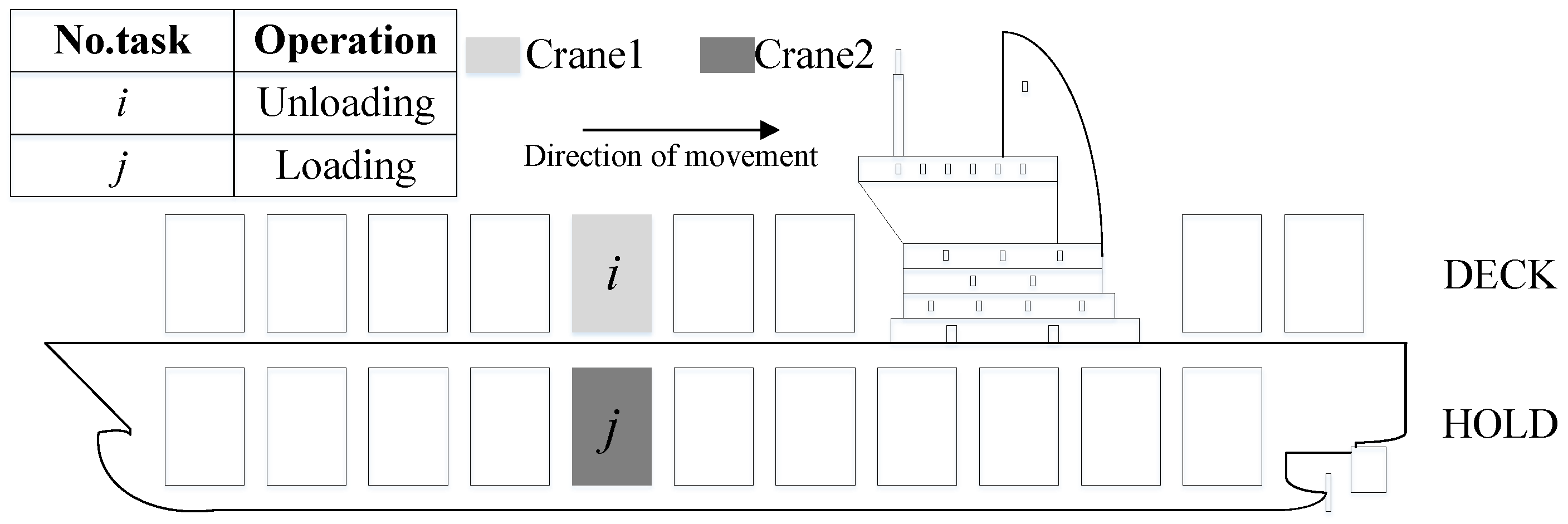
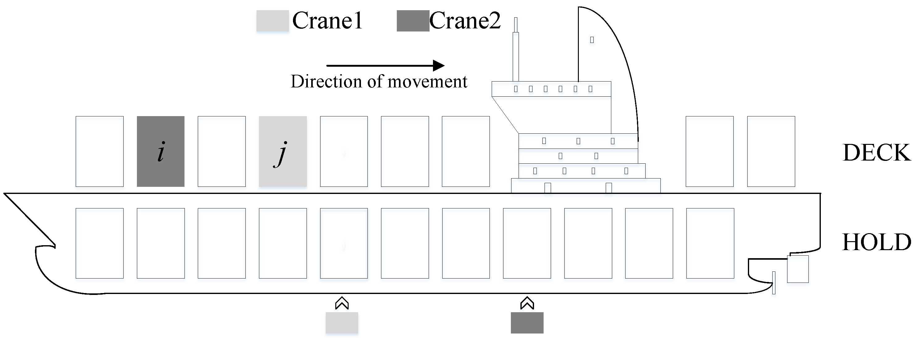
3.1. Quay Crane Scheduling with Energy Consumption

The QCSPEC considers the energy consumption of quay cranes based on the traditional QCSP. It can be defined as follows. Given a set of tasks, Ω = { 1 , 2 , , n } , which locates in the bay B = { 1 , 2 , , m } , and a set of cranes Q = { 1 , 2 , , q } , find a series of Pareto-optimal schedules, such that the vessel completion time (makespan) is shorter and the energy consumption is more economical. Each task i Q denotes a loading or unloading operation of a certain container group, which locates in the bay position b i . Let p i k and e i k , respectively, represent the processing time and energy consumption when task i is operated by the crane k. Let μ k be the energy consumption per unit time of the crane k in a non-working state (waiting or travel). Tasks must be performed by a crane without preemption. In addition, dummy tasks 0 and T with a processing time of 0 and energy consumption (0) are given to indicate the beginning and end of the service of the vessel. Further task sets are defined by Ω 0 = Ω { 0 } , Ω T = Ω { T } , and Ω ¯ = Ω { 0 , T } . Let Φ denote the set of precedence-constrained task pairs, i.e., for each ( i , j ) Φ , task i must be complete before task j starts. Similarly, Let Ψ denote the set of task pairs that cannot be performed at the same time, i.e., for each ( i , j ) Ψ , task i has to precede task j, or task j has to be complete before task i starts. Regarding the cranes, let r k denote the earliest available time of the crane k, and b 0 k denote the starting positions, which are expressed by ship bay numbers. The travel time of crane k between bay positions b i and b j is defined as t i j k = t k × | b i b j | , where t k denotes the travel time of crane k between two adjacent bays.
For safety reasons, adjacent cranes have to keep a safety margin δ , measured in units of bays, at all times. Then, δ v w is the smallest allowed difference between the bay positions of cranes v and w. Furthermore, let Δ i j v w denote the minimum time span to elapse between the processing of two tasks i and j, when processed by cranes v and w, respectively. Let Θ denote the set of all combinations of tasks and cranes that potentially lead to crane interference. Δ i j v w and Θ are defined as follows [13]:
Δ i j v w = ( b i b j + δ v w ) × max { t v , t w } , i j , v < w , b i > b j δ v w ( b j b i + δ v w ) × max { t v , t w } , i j , v > w , b i < b j δ v w 0 , o t h e r w i s e
Θ = { ( i , j , v , w ) Ω 2 × Q 2 | i < j , Δ i j v w > 0 }
As unidirectional scheduling is the preferred strategy for container terminal operations (see, for instance, [15,18]), we also restrict ourselves to the unidirectional QCSP. Furthermore, it is assumed that no two cranes can operate at the same bay at the same time. Meanwhile, as all the cranes travel on the same track, a crane can only serve the next bay without crossing the others. If a crane is needed to cross others, then it must wait until the other crane finishes its tasks and moves away. The parameters and decision variables for the model are summarized in Table 2.

3.2. A Bi-Objective Model

The two objectives are described as OBJ 1 and OBJ 2 below. Among them, the first objective is to minimize the vessel completion time (makespan), and the second one is to minimize the total handling energy consumption of quay cranes.
( QCSPEC ) OBJ 1 = min c m a x
OBJ 2 = k Q i Ω e i k · y i k + k Q ( i , j ) Ω ¯ μ k · ( ϖ i j k + τ i j k )
s . t . j Ω T x 0 j k = 1 k Q
j Ω 0 x i T k = 1 k Q
j Ω T x i j k = y i k k Q , i Ω
j Ω 0 x j i k = y i k k Q , i Ω
k Q y i k = 1 i Ω
y i v 2 y j w d v , w Q , v < w , ( i , j ) Φ
y i w 1 + d y j v v , w Q , v < w , ( i , j ) Φ
z i j y i k + y j k + d 2 k Q , i , j Ω , i < j
z j i 3 y i k y j k d k Q , i , j Ω , i < j
z j i y i k + y j k d 1 k Q , i , j Ω , i < j
z i j 2 + d y i k y j k k Q , i , j Ω , i < j
z i j 3 y i v y j w d v , w Q , v < w , i , j Ω
z j i 2 y i v y j w + d v , w Q , v < w , i , j Ω
y i v + y j w 1 + z i j + z j i ( i , j , v , w ) Θ
c i + k Q p j k · y j k c j 0 ( i , j ) Φ
z i j + z j i = 1 ( i , j ) Ψ
c i + t i j k + p j k c j M ( 1 x i j k ) k Q , i , j Ω
c i + k Q p j k · y j k c j M ( 1 z i j ) i , j Ω
c i + Δ i j v w + p j w · y j w c j M ( 3 z i j y i v y j w ) ( i , j , v , w ) Θ
c j + Δ i j v w + p i v · y i v c i M ( 3 z j i y i v y j w ) ( i , j , v , w ) Θ
ϖ i j k c j p j k · y j k t i j k c i M ( 1 x i j k ) k Q , i , j Ω
τ i j k t i j k M ( 1 x i j k ) k Q , i , j Ω
τ 0 j k t 0 j k M ( 1 x 0 j k ) k Q , j Ω
r k + t 0 j k + p j k · y j k c j M ( 1 x 0 j k ) k Q , j Ω
c i + t i T k c k M ( 1 x i T k ) k Q , i Ω
c k c m a x k Q
The objective function (3) minimizes the completion time of the ship (makespan). The objective function (4) minimizes the cost of total handling energy consumption of cranes during work and idle (waiting and travel) periods. Constraints (5) and (6) ensure, respectively, where each crane k leaves its initial state 0 and ends at its final state T. Constraints (7) and (8) define variables y i k . Constraints (9) ensure that each task is assigned to exactly one crane and constraints (7)–(9) define the flow balance for each task. Constraints (10) and (11) ensure the precedence relationship between tasks and maintain the unidirectional scheduling of cranes. Constraints (12)–(17) define the decision variable z i j . If task i and j ( i < j ) are assigned to crane k, and crane k moves to the right( d = 1 ), then z i j = 1 and z j i = 0 . Conversely, if d = 0 and y i k = 1 and y j k = 1 , then z j i = 1 and z i j = 0 . Constraints (16) and (17) ensure that when two tasks cannot be processed at the same time (task i and j belong to the disjunctive set), a unidirectional scheduling generation scheme gives priority to the crane located in the moving direction. Constraints (18) define the non-crossing requirement among cranes. Constraints (19) guarantee that task i will be processed before task j if there is a precedence relationship between them. Constraints (20) ensure that tasks i and j are not processed simultaneously if ( i , j ) belongs to the non-simultaneous task set. Constraints (21) determine the completion time for each task and eliminate sub-tours. (22) guarantee that task i will be complete before task j if there is a precedent relationship between them. Constraints (23) and (24) avoid crane collisions by inserting the required temporal distance Δ i j v w between the processing of two tasks, considering their processing sequence defined by variables z i j . Constraints (25) determine the waiting time that occurs when a crane has completed task i and will process task j. Constraints (26) define the travel time between task i and task j. Constraints (27) define the travel time of the crane between its initial position and the position of the first task assigned. Constraints (28) restrict the earliest starting time of the operations by each crane. Constraints (29) define the completion time of each crane. Constraints (30) evaluate the makespan.

3.3. A Reinforcement Model

The values of M in QCSPEC can be enforced according to specific constraints. To do so, we first give some notations. Let Φ ( j ) = { i Ω : ( i , j ) Φ } denote a set of tasks that must precede task j, and p i = min k Q { p i k } denote the minimum processing time of cranes for task i. The lower bound on the starting time of a task j can be estimated by
a j = max min k Q { r k + t 0 j k } , max i Φ ( j ) { a i + p i } .
Moreover, let u denote the upper bound for the makespan if only one crane performs all loading and unloading operations:
u = min k Q r k + i Ω p i k + t 0 T k .
With these notations in hand, we can present a reinforcement model for QCSPEC, where it has the same objective functions (3)–(4) and is subject to the following constraints:
   (5)–(20), (30)
c i + t i j k + p j k c j M i j k 1 ( 1 x i j k ) k Q , i , j Ω
c i + k Q p j k · y j k c j M i j 2 ( 1 z i j ) i , j Ω
c i + Δ i j v w + p j w · y j w c j M i j v w 3 ( 3 z i j y i v y j w ) ( i , j , v , w ) Θ
c j + Δ i j v w + p i v · y i v c i M i j v w 4 ( 3 z j i y i v y j w ) ( i , j , v , w ) Θ
ϖ i j k c j p j k · y j k t i j k c i M i j k 5 ( 1 x i j k ) k Q , i , j Ω
τ i j k t i j k M i j k 6 ( 1 x i j k ) k Q , i , j Ω
τ 0 j k t 0 j k M j k 7 ( 1 x 0 j k ) k Q , j Ω
r k + t 0 j k + p j k · y j k c j M j k 8 ( 1 x 0 j k ) k Q , j Ω
c i + t i T k c k M i k 9 ( 1 x i T k ) k Q , i Ω
where M i j k 1 = u + t i j k a j , M i j 2 = u a j , M i j v w 3 = u + Δ i j v w a j , M i j v w 4 = u + Δ i j v w a i , M i j k 5 = u p j t i j k a i , M i j k 6 = t i j k , M j k 7 = t 0 j k , M j k 8 = r k + t 0 j k a j , M i k 9 = u + t i T k r k .

4. Solution Method

The QCSPEC is a complicated bi-objective optimization problem. To tackle this issue, a branch-and-bound algorithm (BaB) is presented to find the Pareto-optimal solutions. In the following, we describe all necessary problem-dependent parts of the algorithm.

4.1. Lexicographical Sorting

For convenience, we assume that all cranes are indexed sequentially according to increasing positions alongside the quay. Similarly, we assume that the tasks are ordered lexicographically in increasing bay positions, and for tasks within the same bay, the order is determined by considering the precedence relationship between tasks. In the following sections, a unique lexicographical sorting of tasks is supposed to be given.

4.2. Lower Bounds

We present several lower bounds for BaB to decide whether the current node in the search tree is pruned or not. Because QCSPEC involves the comparison of two dimensions, we propose different lower bounds for makespan and energy consumption, respectively. If the current node is dominated, the corresponding subtree connected to that node is no longer explored. It should be pointed out that some of the lower bounds related to the makespan have been refined from previous papers (see, for instance, [13,15,16,45]).

4.2.1. Lower Bounds for OBJ 1

(Lower Bound 1). The first lower bound evaluates the estimated crane completion time and the minimum completion time that can be achieved if the unassigned tasks are perfectly assigned to cranes. This is an ideal assignment and, therefore, can be used as a reasonable lower bound:
L B ( t ) 1 = max max k Q c ˜ k , k Q c ˜ k + i Ω u min k Q p i k / q ,
where c ˜ k is the earliest estimated completion time of crane k and Ω u is the set of so far unassigned tasks in the enumeration tree. Specifically, c ˜ k is computed as:
c ˜ k = r k + i Ω k p i k + b 0 k b l o k + b u p k b l 0 k · t k ,
where b l o k and b u p k are the lowest bay and utmost bay visited by crane k of the current node in the enumeration tree, respectively, and Ω k is the set of tasks currently assigned to crane k, i.e., Ω k = { i Ω | y i k = 1 } . In particular, for unidirectional schedules, the total travel time of a crane is given by its initial bay position b l 0 k , the lowest bay b l o k , and the utmost bay b u p k it had visited in the current search tree. Note that L B ( t ) 1 gives a most relaxed form of the lower bound function.
(Lower Bound 2). The second lower bound contains the estimated minimum travel time required for the crane to move from its current position to all unassigned tasks.
L B ( t ) 2 = max max k Q c ˜ k , k Q c ˜ k + i Ω u min k Q p i k + L B T T / q ,
where the term L B T T denotes the estimated minimum travel time required to perform unassigned tasks. Let B = { b 1 , b 2 , . . . ; b m } donates the set of bay locations and contains the current positions of cranes in the search tree and the positions of unassigned tasks (i.e., l i B , i Ω u ). Without loss of generality, the elements in B are sorted in lexicographical order. The term L B T T can be obtained by:
L B T T = t l + t r + t b
where the term t l is the minimum travel time required by the left-most crane to perform the left-most task, t r is that required to handle the unassigned right-most task by the current right-most crane, and t b is the lower bound on the travel time of all adjacent cranes. Moreover, B can be divided into q 1 partitions based on the bay index of cranes. For an interval [ l k , l k + 1 ] , if there is at least one unassigned task i Ω u in this interval, we can derive the term t b by:
t b = k = 1 k = q 1 l k + 1 l k max i [ l k , l k + 1 ] l i + 1 l i · max { t k , t k + 1 } .
Note that L B ( t ) 2 takes into account the travel time between unassigned tasks. Therefore, L B ( t ) 2 is more powerful than L B ( t ) 1 , while additional computational effort is required.
(Lower Bound 3). The third lower bound takes into account the non-working weight of the crane, which is restricted by non-crossing and safe distance constraints.
L B ( t ) 3 = max max v Q c ˜ v + max k = v + 1 , . . . , q { b v k } , max k Q v Q c ˜ v + v = 1 k 1 b v k + j Ω u min v Q { p j v } + L B T T / q ,
where b v k is the blockage time of crane v by crane k (with v < k ). For a node at level n of the search tree, b v k is the minimum blockage period of crane v provided by crane k. Therefore, the first term in (47) is a lower bound on the completion of crane v. The second term in (47) considers the block time. To be precise, let c ˜ k and c ˜ v denote the earliest estimated completion times of cranes k and v, respectively. If the completion time of crane v is earlier than the ready time of crane k, crane v will be blocked for a length of time r k c ˜ v . If crane v’s earliest estimated completion time is earlier than crane k but later than the ready time of crane k ( r k < c ˜ v < c ˜ k ), crane v has to wait until crane k finishes its service. Considering the above two situations, the blockage time of crane v by crane k is given by:
b v k = c ˜ k c ˜ v , i f r k c ˜ v c ˜ k c ˜ k r k , i f c ˜ v < r k < c ˜ k 0 , o t h e r w i s e
Remark that L B ( t ) 3 makes good use of the lexicographical sorting of tasks, ensuring that the unassigned tasks are above the assigned tasks, so they can provide tighter lower bounds than L B ( t ) 2 .

4.2.2. Lower Bounds for
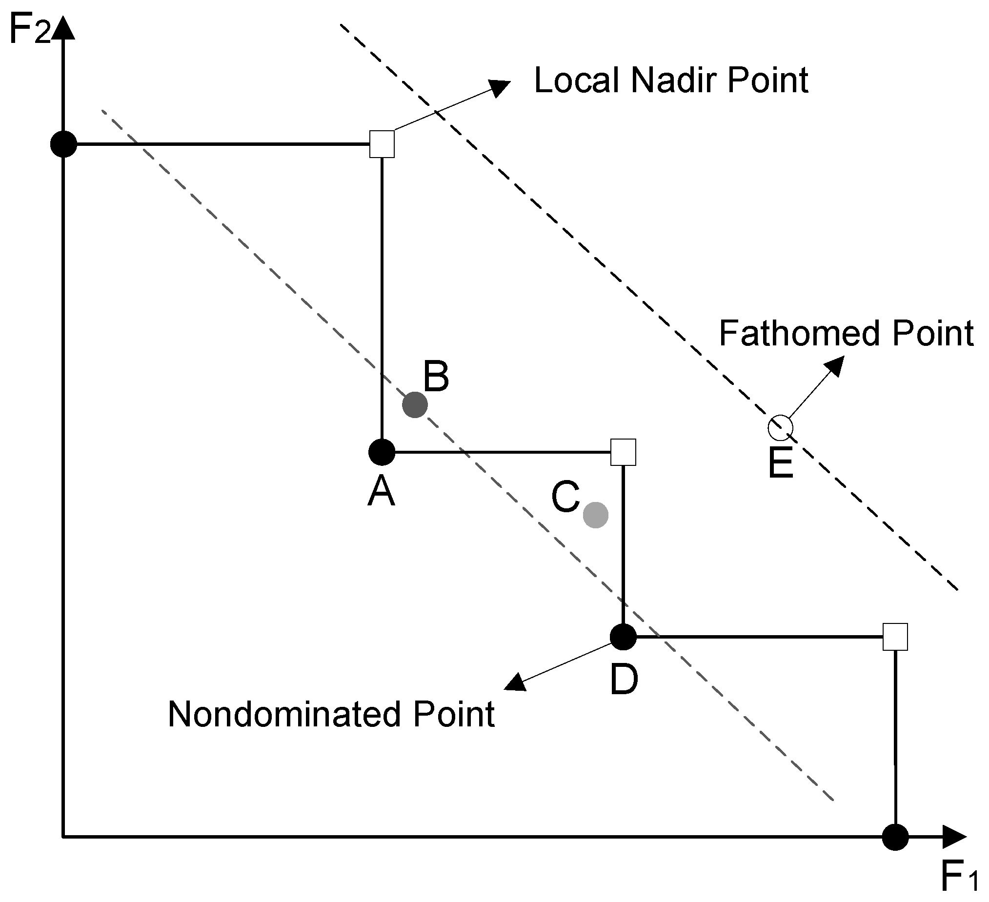
 OBJ 2

In QCSPEC, each task has two attributes, namely time and energy. In the following, we introduce how to obtain the lower bounds on energy consumption.
(Lower Bound 1). The first lower bound for energy consumption corresponds to L B ( t ) 1 , under the assumption that no extra energy is consumed during handling operations. The energy consumption of crane k can be estimated by
g ˜ k = i Ω k e i k + | b 0 k b l o k | + | b u p k b l 0 k | · μ k .
Then, the first lower bound for energy consumption is
L B ( e ) 1 = k Q g ˜ k + i Ω u min k Q e i k .
Note that L B ( e ) 1 describes an ideal condition in which unassigned tasks are processed with minimal energy, regardless of the energy consumption of the blockage. It can quickly give a lower bound on energy consumption with a small amount of computation.
(Lower Bound 2). This bound takes into account the travel energy of cranes that service unassigned tasks. Similar to L B T T , we propose a term called L B T E to describe this part of energy consumption. Based on the definition of L B T T , we can easily derive L B T E by
L B T E = g l + g r + g b ,
where g l and g r are the minimal energy consumption of cranes to move to the left- and right-most tasks and g b represents the minimum energy required to service tasks located between all adjacent cranes:
g b = k = 1 k = q 1 l k + 1 l k max i [ l k , l k + 1 ] l i + 1 l i · μ k .
We can then derive the second lower bound by
L B ( e ) 2 = k Q g ˜ k + i U min k Q e i k + L B T E .
(Lower Bound 3). A further condition to enhance the lower bound is obtained from considering the possible blocking of the cranes. The energy consumption when the crane is blocked is related to the blocking time, so we can directly obtain the energy consumption during this period after deriving the blocking time, i.e., b v k × μ v . Therefore, the third lower bound can be expressed as:
L B ( e ) 3 = max v Q g ˜ v + max k = v + 1 , . . . , q b v k · μ v , max k Q v Q g ˜ v + v = 1 k 1 b v k · μ v + j U min v Q e j v + L B T E .

4.3. Upper Bounds

To obtain a tight upper bound at the root node, we used three initial solution strategies, namely S-TASKS, S-LOAD, and SCD, which were proposed by Sammarra et al. [46] and Legato and Trunfio [16]. S-TASKS constructs an initial solution by dividing the tasks Ω into | Q | parts to ensure that the number of tasks assigned to each crane is approximately the same. S-LOAD constructs an initial solution by assigning approximately the same amount of workload (in terms of task processing time) to each crane. SCD considers the safety distance and non-crossing requirements of the crane when constructing the initial solution, the goal of which is to minimize the delay (waiting) of the crane. For the QCSPEC, the initial solution with the shortest makespan among the three strategies will be the best initial solution for the first goal, while the initial solution for the second goal selects the one with the lowest energy consumption.

4.4. Branching Criteria

If a solution cannot be dominated, the BaB algorithm applies two branching criteria, ensuring the construction of a unidirectional schedule by restricting the inspection of search tree.
(Branching Criterion 1). The first branching criterion is the one proposed by Bierwirth and Meisel [13]. Consider two tasks, i and j, which have a precedence relationship (i.e., ( i , j ) Φ ). In order to guarantee the unidirectional movements of cranes, the following constraints need to be satisfied:
q i q j ( i , j ) Φ
In Figure 1, we give a situation where constraint (55) may be violated. It can be found that task j can only be assigned to crane 1 if task i is assigned to crane 1, otherwise the constraints of the unidirectional movements of cranes cannot be guaranteed. Similarly, if crane 2 operates task i, then task j will be able to be assigned to crane 1 or to crane 2.
This branching criterion avoids considering branches that would cause the crane to change the direction of motion. In addition, the number of branches in the search tree can be greatly reduced due to the existence of the precedence relationship.
(Branching criterion 2). The second branching criterion considers how to assign the first task to cranes. Consider two adjacent cranes v and w ( v < w ), which have not been assigned tasks yet. Task i cannot be assigned to crane w if the following branching criterion holds:
r v + t 0 i v < r w + t 0 i w .
This branching criterion means that we should assign tasks to a crane that can start as soon as possible, which is more in line with the actual operation and will enable task i to be completed earlier, and avoid the idle of cranes. This branching rule also reduces the number of branches in the search tree, especially at the first few nodes. Figure 2 depicts the effectiveness of this branching criterion. In this case, if task i is assigned to crane 2, crane 1 must move downward to stay idle.

4.5. Fathoming Criterion

Given the feasible schedule, such as the classical branch-and-bound algorithm, the BaB algorithm attempts to fathom the solution. The difference is that the incumbent in the BaB algorithm is not one solution but a set of non-dominated points. Following this idea, we now consider a solution B (shown in Figure 3) with two objective function values, f 1 and f 2 , respectively. Even if it is actually dominated by an existing solution A in the current set of non-dominant points, solution B cannot be fathomed because there could be another later solution (solution C) that is dominated by solution B, but is a part of the non-dominant points (see Figure 3). In the BaB algorithm, we determine whether the solution is fathomed by comparing the two objective function values of the current solution with the objective function values of all local nadir points (see Definition 1 for details). Specifically, the set of non-dominated points is depicted in Figure 3. Intuitively, solution B cannot be fathomed, but solution E can.
Definition 1. 
(Local Nadir point). Given a set of non-dominated points Z , a point is called local nadir point between each pair of points F ( σ i ) and F ( σ i + 1 ) in Z , such that F l o c a l   n a d i r = ( F 1 ( σ i + 1 ) , F 2 ( σ i ) ) , where F 1 ( · ) and F 2 ( · ) denote the first and second objective values of a given schedule, respectively.
In BaB, given a feasible schedule σ , which we need to check whether it can be bounded, if F 1 ( σ ) + F 2 ( σ ) > max i Z ( F 1 ( σ i + 1 ) + F 2 ( σ i ) ) , then we can fathom point F ( σ ) . Note that this fathoming criterion requires normalizing the two objective function values; see Definition 2.
Definition 2. 
(Normalization). Let F U L and F L R denote the upper left and the lower right points, respectively. Given the two corner points F U L and F L R , we can easily derive the ideal point F i d e a l and the nadir point F n a d i r . Further, we can normalize the points in the non-dominated set Z by:
F 1 ( σ ) = F 1 ( σ ) F 1 U L F 1 L R F 1 U L , F 2 ( σ ) = F 2 ( σ ) F 2 L R F 2 U L F 2 L R .

5. Results

In this section, we first show how the model and algorithm work on an illustrative example. We then conduct a series of simulation experiments to compare the proposed branch-and-bound algorithm with other approaches.

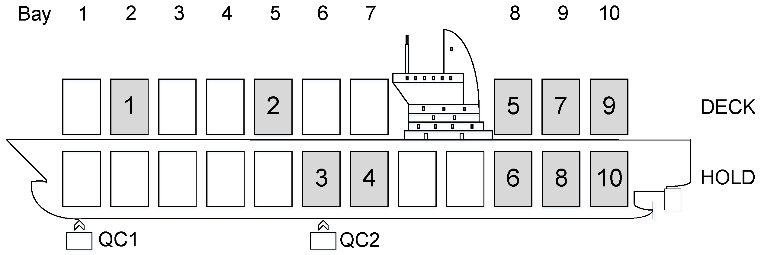
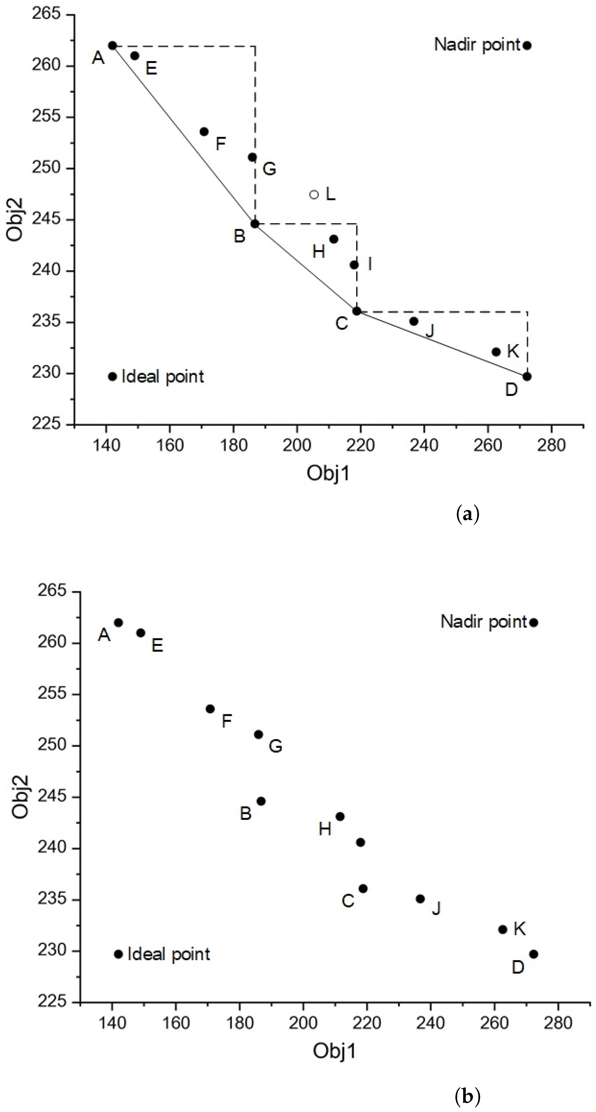
5.1. An Illustrative Case Study

We now demonstrate the usefulness of our bi-objective quay crane scheduling model with time-saving and energy-saving on an illustrative example problem. We use the simulated data presented in Table 3. In this example, n = 10 container groups have to be processed for a ship of size m = 10 bays, which is operated by q = 2 cranes. The safety margin between cranes is set to δ = 1 , and the cranes can move from one bay to an adjacent bay. Furthermore, Figure 4 shows the discharge/loading workloads for quay crane operations.
We solve the above example by our bi-objective branch-and-bound method and illiterate the non-dominated points and Pareto-optimal front in Figure 5. Note that there are 11 non-dominated points. The container terminal operator can choose one of the scheduled plans based on the operational targets. Specifically, if the operator prefers a time-efficient plan, she/he could apply the schedule corresponding to point A, which is able to achieve the shortest makespan. On the other hand, when energy and emission reductions dominate, they can take option D. As a result, they can minimize the total energy consumption (thereby leading to emission reduction). Moreover, our proposed bi-objective branch-and-bound method for the quay crane scheduling problem has access to all non-dominated points in the criterion space.
One may argue that such a Pareto-optimal front can also be obtained by a weighted sum version. More precisely, one can adjust the weight of each objective and keep the weighted sum equal to one. We would like to clarify that the application of the weighted sum method depends on the setting of the weights, which is difficult for port operation practice. In general, time-saving and energy-saving are usually not of an order of magnitude, so it is difficult to compare to determine weights. The bi-objective branch-and-bound method, however, gives a global view of the full Pareto-optimal front, where every point is non-dominated. Therefore, decision-makers can make a choice from the Pareto-optimal front based on their decision preference, while they also know the performances of other scheduling schemes.
After obtaining the Pareto-optimal front, we can use the non-numerical ranking preferences method (NRPM) [47] for the post-Pareto analysis. To do so, instead of using weights, the decision-maker only needs to perform a non-numerical ordering of the objectives. Finally, by combining the branch-and-bound algorithm with the NRPM method, we can obtain a decision support tool for quay crane scheduling considering the time- and energy-savings at the container terminals.

5.2. Simulation Experiment

5.2.1. Generation of the Test Instances

We generated four instance sets of different sizes with 10 instances, each to examine the computational efficiency of the proposed branch-and-bound algorithm. Specifically, the number of tasks was set to n = { 10 , 15 , 20 , 25 } , the total number of cranes was equal to q = { 2 , 3 } , and the number of ship-bays was the same as the number of tasks, i.e., m = { 10 , 15 , 20 , 25 } . Moreover, the processing time and energy consumption for a task were randomly generated from uniform distributions U(3,100) and U(10,100), respectively. It was assumed that the initial positions of the cranes were equally spaced on the ship, and the ready times of all cranes were set to zero. The travel time and non-working energy consumption of cranes were assumed to follow uniform distributions U(0.5,1.5), and the safety distance was set to one bay in all instances. The parameters used to generate the instances are listed in Table 4.

5.2.2. Quality of Lower Bounds

In this section, our goal is to demonstrate the computational effectiveness of the lower bounds for the branch-and-bound algorithm in Section 4.2. We denote BaB [ i ] to be the branch-and-bound algorithm with lower bounds up to i { i , 2 , 3 } . For example, BaB [ 3 ] represents the branch-and-bound algorithm with lower bounds 1, 2, and 3. The mean and standard deviations of the solution times of the corresponding three algorithms over the test instances are reported in Figure 6. We notice several advantages of the branch-and-bound algorithm with more lower bounds: (1) The lower bounds can bring about a reduction in the computation time. (2) The fluctuations in computation times generally decrease as more lower-bound functions are used.

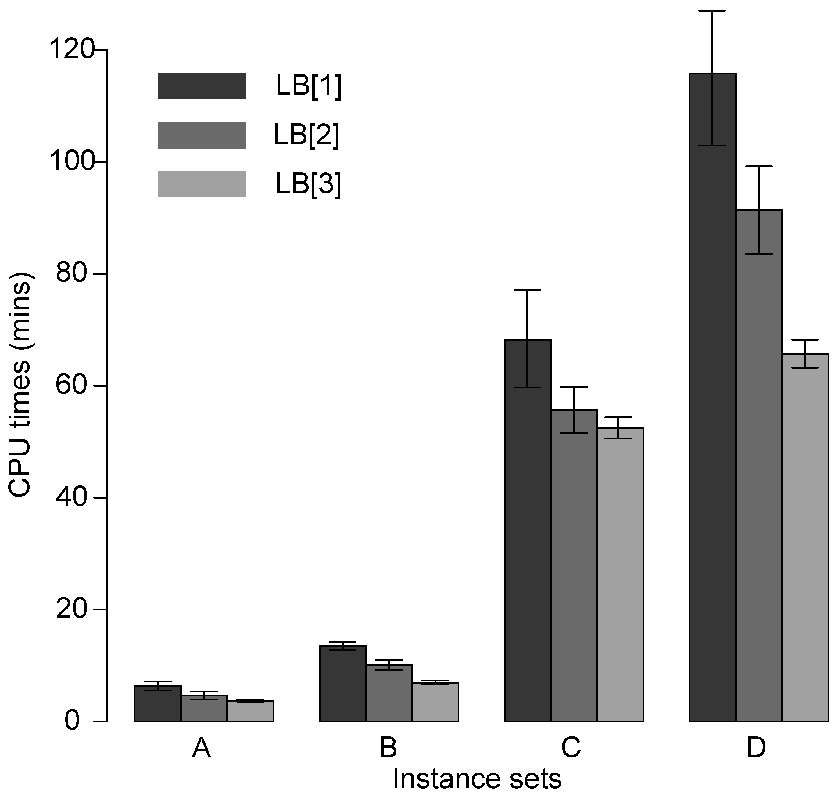
5.2.3. Performance Comparison

We examine the performance of the branch-and-bound algorithm in terms of solution quality and computational tractability. Specifically, we benchmark the branch-and-bound algorithm against two approaches that solve bi-objective problems: (1) the ϵ -constraint method by Chankong and Haimes [48] that is an exact solution approach, and (2) multi-objective particle swarm optimization (MOPSO) by Coello et al. [49], which is a heuristics-based solution methodology. We refer interested readers to these references for more details. In our implementation, we applied CPLEX for the exact solution processes required in the ϵ -constraint, and an open-source MATLAB package [50] for MOPSO. We set the time limit to solve bi-objective problems to two hours (120 min).
To evaluate the performance of different bi-objective solution approaches, we defined a metric “ratio of Pareto-front” (RoP) by the number of non-dominated solutions found in the percentage, from the whole set of Pareto-optimal solutions. In Table 5, we summarize the RoP and computation time under the following approaches: the branch-and-bound algorithm (BaB), the ϵ -constraint method, and the MOPSO. Our numerical experiments on test instances suggest that the BaB outperforms the ϵ -constraint and MOPSO in terms of solution quality. Specifically, the BaB brings significant RoP, greater than or equal to the other two approaches, while the ϵ -constraint becomes intractable as the problem size increases (e.g., n 20 ). Moreover, the ability of the MOPSO to explore the Pareto-optimal front decreases as it deals with larger instances. When it comes to computational time, heuristics-based MOPSO takes the least amount of time, followed by BaB, and finally the ϵ -constraint. The reason is that the BaB and the ϵ -constraint focus on identifying the whole set of Pareto-optimal solutions for bi-objective problems. We do believe that there is still room to improve the BaB by developing additional acceleration schemes. This constitutes a natural direction for future research.

6. Conclusions

This study focused on the quay crane scheduling problem, which addresses the transshipment of containers between ships and cranes. Specifically, QCSP consists of determining the sequence of operations of cranes assigned to a ship, with respect to a given objective function. The objective of QCSP is to minimize the ship’s completion time. However, the container terminal also needs to pay attention to other goals, such as energy consumption while improving handling efficiency. To deal with the trade-off between efficiency and energy consumption (and, thereby reducing emissions), we formulated a bi-objective mixed-integer programming model with the objective of minimizing the service time of vessels and the energy consumption of cranes. Mathematically, we designed a branch-and-bound algorithm to identify the full set of Pareto-optimal solutions. We also proposed various lower/upper bounds and branching/fathoming criteria to make the algorithm more efficient. We showed how the model and algorithm work on an illustrative example, which demonstrates the value of using the proposed branch-and-bound algorithm for the bi-objective QCSP. A comparison with other algorithms on an extensive set of simulation instances illustrated the effectiveness of the proposed algorithm in terms of computational tractability and solution quality. Empirically, our branch-and-bound algorithm can handle small- and medium-sized problems efficiently, which can provide the benchmarking of heuristics. Hence, developing metaheuristics for large problems would constitute a natural direction for future research.

Author Contributions

Writing—original draft preparation, H.L.; writing—review and editing, X.L. and H.L.; funding acquisition, X.L.; formal analysis, H.L. All authors have read and agreed to the published version of the manuscript.

Funding

This research was funded by the National Social Science Foundation of China, grant no. 21CZZ007, the Tianjin Social Science Foundation of China, grant no. TJGLQN20-001, China Postdoctoral Science Foundation, grant no. 2020M670636, and the Liberal Arts Development Foundation of Nankai University, grant no. ZB22BZ0332.

Institutional Review Board Statement

Not applicable.

Informed Consent Statement

Not applicable.

Data Availability Statement

Not applicable.

Acknowledgments

The authors thank Ning Zhu and Shoufeng Ma for the helpful discussions and feedback.

Conflicts of Interest

The authors declare no conflict of interest.

Abbreviations

The following abbreviations are used in this manuscript:
BaBbranch-and-bound
GHGgreenhouse gas
IMOInternational Maritime Organization
MILPmixed integer linear programming
MOPSOmulti-objective particle swarm optimization
NRPMnon-numerical ranking preferences method
QCSPquay crane scheduling problem
QCSPECquay crane scheduling problem with energy consumption
TEUtwenty-foot equivalent unit

References

  1. UNCTAD. Review of Maritime Transport 2021. 2021. Available online: https://unctad.org/system/files/official-document/rmt2021_en_0.pdf (accessed on 1 January 2022).
  2. Kong, L.; Ji, M.; Gao, Z. An exact algorithm for scheduling tandem quay crane operations in container terminals. Transp. Res. Part E Logist. Transp. Rev. 2022, 168, 102949. [Google Scholar] [CrossRef]
  3. Yue, L.; Fan, H. Dynamic Scheduling and Path Planning of Automated Guided Vehicles in Automatic Container Terminal. IEEE/CAA J. Autom. Sin. 2022, 9, 2005–2019. [Google Scholar] [CrossRef]
  4. Yan, S.y.; Wang, C.Y.; Wei, C.S. Manpower supply planning for routine policing duties. J. Chin. Inst. Eng. 2022, 45, 669–678. [Google Scholar] [CrossRef]
  5. Pinedo, M.L. Scheduling; Springer: Berlin/Heidelberg, Germany, 2012; Volume 29. [Google Scholar]
  6. UNCTAD. Third IMO Greenhouse Gas Study 2014. 2014. Available online: https://www.escholar.manchester.ac.uk/api/datastream?publicationPid=uk-ac-man-scw:266097&datastreamId=FULL-TEXT.PDF (accessed on 1 January 2022).
  7. Villalba, G.; Gemechu, E.D. Estimating GHG emissions of marine ports—The case of Barcelona. Energy Policy 2011, 39, 1363–1368. [Google Scholar] [CrossRef]
  8. Liu, D.; Ge, Y.E. Modeling assignment of quay cranes using queueing theory for minimizing CO2 emission at a container terminal. Transp. Res. Part D Transp. Environ. 2018, 61, 140–151. [Google Scholar] [CrossRef]
  9. Daganzo, C.F. The crane scheduling problem. Transp. Res. Part B Methodol. 1989, 23, 159–175. [Google Scholar] [CrossRef]
  10. Bierwirth, C.; Meisel, F. A survey of berth allocation and quay crane scheduling problems in container terminals. Eur. J. Oper. Res. 2010, 202, 615–627. [Google Scholar] [CrossRef]
  11. Bierwirth, C.; Meisel, F. A follow-up survey of berth allocation and quay crane scheduling problems in container terminals. Eur. J. Oper. Res. 2015, 244, 675–689. [Google Scholar] [CrossRef]
  12. Liu, J.; Wan, Y.w.; Wang, L. Quay crane scheduling at container terminals to minimize the maximum relative tardiness of vessel departures. Nav. Res. Logist. (NRL) 2006, 53, 60–74. [Google Scholar] [CrossRef]
  13. Bierwirth, C.; Meisel, F. A fast heuristic for quay crane scheduling with interference constraints. J. Sched. 2009, 12, 345–360. [Google Scholar] [CrossRef]
  14. Meisel, F. The quay crane scheduling problem with time windows. Nav. Res. Logist. (NRL) 2011, 58, 619–636. [Google Scholar] [CrossRef]
  15. Legato, P.; Trunfio, R.; Meisel, F. Modeling and solving rich quay crane scheduling problems. Comput. Oper. Res. 2012, 39, 2063–2078. [Google Scholar] [CrossRef]
  16. Legato, P.; Trunfio, R. A local branching-based algorithm for the quay crane scheduling problem under unidirectional schedules. 4OR 2014, 12, 123–156. [Google Scholar] [CrossRef]
  17. Chen, J.H.; Lee, D.H.; Goh, M. An effective mathematical formulation for the unidirectional cluster-based quay crane scheduling problem. Eur. J. Oper. Res. 2014, 232, 198–208. [Google Scholar] [CrossRef]
  18. Chen, J.H.; Bierlaire, M. The study of the unidirectional quay crane scheduling problem: Complexity and risk-aversion. Eur. J. Oper. Res. 2017, 260, 613–624. [Google Scholar] [CrossRef]
  19. Ma, S.; Li, H.; Zhu, N.; Fu, C. Stochastic programming approach for unidirectional quay crane scheduling problem with uncertainty. J. Sched. 2021, 24, 137–174. [Google Scholar] [CrossRef]
  20. Xia, J.; Wang, K.; Wang, S. Drone scheduling to monitor vessels in emission control areas. Transp. Res. Part B Methodol. 2019, 119, 174–196. [Google Scholar] [CrossRef]
  21. Lai, X.; Ng, C.T.; Wan, C.L.J. Bi-objective evacuation problem in ships or buildings. Int. J. Shipp. Transp. Logist. 2022, 14, 172–192. [Google Scholar] [CrossRef]
  22. Psaraftis, H.N.; Kontovas, C.A. Speed models for energy-efficient maritime transportation: A taxonomy and survey. Transp. Res. Part C Emerg. Technol. 2013, 26, 331–351. [Google Scholar] [CrossRef]
  23. Mansouri, S.A.; Lee, H.; Aluko, O. Multi-objective decision support to enhance environmental sustainability in maritime shipping: A review and future directions. Transp. Res. Part E Logist. Transp. Rev. 2015, 78, 3–18. [Google Scholar] [CrossRef]
  24. Chang, D.; Jiang, Z.; Yan, W.; He, J. Integrating berth allocation and quay crane assignments. Transp. Res. Part E Logist. Transp. Rev. 2010, 46, 975–990. [Google Scholar] [CrossRef]
  25. Esmemr, S.; Ceti, I.B.; Tuna, O. A Simulation for Optimum Terminal Truck Number in a Turkish Port Based on Lean and Green Concept. Asian J. Shipp. Logist. 2010, 26, 277–296. [Google Scholar] [CrossRef] [Green Version]
  26. Chen, G.; Govindan, K.; Golias, M.M. Reducing truck emissions at container terminals in a low carbon economy: Proposal of a queueing-based bi-objective model for optimizing truck arrival pattern. Transp. Res. Part E Logist. Transp. Rev. 2013, 55, 3–22. [Google Scholar] [CrossRef]
  27. He, J.; Huang, Y.; Yan, W. Yard crane scheduling in a container terminal for the trade-off between efficiency and energy consumption. Adv. Eng. Inform. 2015, 29, 59–75. [Google Scholar] [CrossRef]
  28. He, J.; Huang, Y.; Yan, W.; Wang, S. Integrated internal truck, yard crane and quay crane scheduling in a container terminal considering energy consumption. Expert Syst. Appl. 2015, 42, 2464–2487. [Google Scholar] [CrossRef]
  29. He, J. Berth allocation and quay crane assignment in a container terminal for the trade-off between time-saving and energy-saving. Adv. Eng. Inform. 2016, 30, 390–405. [Google Scholar] [CrossRef]
  30. Sha, M.; Zhang, T.; Lan, Y.; Zhou, X.; Qin, T.; Yu, D.; Chen, K. Scheduling optimization of yard cranes with minimal energy consumption at container terminals. Comput. Ind. Eng. 2017, 113, 704–713. [Google Scholar] [CrossRef]
  31. Tan, C.; Yan, W.; Yue, J. Quay crane scheduling in automated container terminal for the trade-off between operation efficiency and energy consumption. Adv. Eng. Inform. 2021, 48, 101285. [Google Scholar] [CrossRef]
  32. Ehrgott, M.; Wiecek, M.M. Mutiobjective Programming. In Multiple Criteria Decision Analysis: State of the Art Surveys; Springer New York: New York, NY, USA, 2005; pp. 667–708. [Google Scholar]
  33. Leitner, M.; Ljubić, I.; Sinnl, M. A Computational Study of Exact Approaches for the Bi-Objective Prize-Collecting Steiner Tree Problem. INFORMS J. Comput. 2015, 27, 118–134. [Google Scholar] [CrossRef]
  34. Boland, N.; Charkhgard, H.; Savelsbergh, M. A criterion space search algorithm for biobjective integer programming: The balanced box method. INFORMS J. Comput. 2015, 27, 735–754. [Google Scholar] [CrossRef]
  35. Parragh, S.N.; Tricoire, F. Branch-and-bound for bi-objective integer programming. INFORMS J. Comput. 2019, 31, 805–822. [Google Scholar] [CrossRef]
  36. Glize, E.; Jozefowiez, N.; Ngueveu, S.U. An ε-constraint column generation-and-enumeration algorithm for Bi-Objective Vehicle Routing Problems. Comput. Oper. Res. 2022, 138, 105570. [Google Scholar] [CrossRef]
  37. Haimes, Y. On a bicriterion formulation of the problems of integrated system identification and system optimization. IEEE Trans. Syst. Man Cybern. 1971, 1, 296–297. [Google Scholar]
  38. Mavrotas, G. Effective implementation of the ε-constraint method in multi-objective mathematical programming problems. Appl. Math. Comput. 2009, 213, 455–465. [Google Scholar] [CrossRef]
  39. Ehrgott, M.; Ruzika, S. Improved ε-constraint method for multiobjective programming. J. Optim. Theory Appl. 2008, 138, 375–396. [Google Scholar] [CrossRef]
  40. Mavrotas, G.; Diakoulaki, D. A branch and bound algorithm for mixed zero-one multiple objective linear programming. Eur. J. Oper. Res. 1998, 107, 530–541. [Google Scholar] [CrossRef]
  41. Mavrotas, G.; Diakoulaki, D. Multi-criteria branch and bound: A vector maximization algorithm for mixed 0-1 multiple objective linear programming. Appl. Math. Comput. 2005, 171, 53–71. [Google Scholar] [CrossRef]
  42. Vincent, T.; Seipp, F.; Ruzika, S.; Przybylski, A.; Gandibleux, X. Multiple objective branch and bound for mixed 0-1 linear programming: Corrections and improvements for the biobjective case. Comput. Oper. Res. 2013, 40, 498–509. [Google Scholar] [CrossRef]
  43. Stidsen, T.; Andersen, K.A.; Dammann, B. A Branch and Bound Algorithm for a Class of Biobjective Mixed Integer Programs. Manag. Sci. 2014, 60, 1009–1032. [Google Scholar] [CrossRef]
  44. Halffmann, P.; Schäfer, L.E.; Dächert, K.; Klamroth, K.; Ruzika, S. Exact algorithms for multiobjective linear optimization problems with integer variables: A state of the art survey. J.-Multi-Criteria Decis. Anal. 2022, 29, 341–363. [Google Scholar] [CrossRef]
  45. Kim, K.H.; Park, Y.M. A crane scheduling method for port container terminals. Eur. J. Oper. Res. 2004, 156, 752–768. [Google Scholar] [CrossRef]
  46. Sammarra, M.; Cordeau, J.F.; Laporte, G.; Monaco, M.F. A tabu search heuristic for the quay crane scheduling problem. J. Sched. 2007, 10, 327–336. [Google Scholar] [CrossRef]
  47. Taboada, H.A.; Coit, D.W. Multi-objective scheduling problems: Determination of pruned Pareto sets. IIE Trans. 2008, 40, 552–564. [Google Scholar] [CrossRef]
  48. Chankong, V.; Haimes, Y.Y. Multiobjective Decision Making: Theory and Methodology; Courier Dover Publications: Mineola, NY, USA, 2008. [Google Scholar]
  49. Coello, C.A.C.; Pulido, G.T.; Lechuga, M.S. Handling multiple objectives with particle swarm optimization. IEEE Trans. Evol. Comput. 2004, 8, 256–279. [Google Scholar] [CrossRef]
  50. Yarpiz. Mostapha Kalami Heris, Multi-Objective PSO in MATLAB. 2015. Available online: https://yarpiz.com/59/ypea121-mopso (accessed on 1 January 2022).
Figure 1. Example of the violation of branching criterion 1.
Mathematics 10 04705 g001
Figure 2. Example of the violation of the branching criterion 2.
Mathematics 10 04705 g002
Figure 3. An example of fathoming criterion.
Mathematics 10 04705 g003
Figure 4. Distribution of quay crane scheduling workload.
Mathematics 10 04705 g004
Figure 5. Optimal solution for the example instance. (a) Nondominated points. (b) Pareto-optimal front.
Mathematics 10 04705 g005
Figure 6. Average computational time of the BaB algorithm with different lower bounds.
Mathematics 10 04705 g006
Table 1. Summary of the literature on energy saving and emission reduction at the port’s operation level 1.
LiteratureProblemObjectiveMethod
Chang et al. [24]BAP & QCAPTime & EnergyWeighted sum
Chen et al. [26]TAPTime & EmissionsHeuristics
He et al. [27]YCSPTime & EnergyWeighted sum
He et al. [28]ISPTime & EnergyWeighted sum
He [29]BAP & QCAPTime & EnergyWeighted sum
Sha et al. [30]YCSPEnergyData fitting
Liu and Ge [8]QCAPEmissionsQueuing
Tan et al. [31]AQCSPTime & EnergyWeighted sum
This paperQCSPTime & EnergyBaB
1 Abbreviations used in this table: BAP—berth allocation problem, QCAP—quay crane assignment problem, TAP—truck arrival pattern, YCSP—yard crane scheduling problem, ISP—integrated scheduling problem, AQCSP—automated quay crane scheduling problem, QCSP—quay crane scheduling problem, BaB—branch-and-bound.
Table 2. Notation.
Table 2. Notation.
Indices
i , j Indices of tasks, which are ordered in increasing order of their relative locations in the direction of ship bay indices
k , v , w Index of quay cranes, which are also ordered in increasing order of their relative locations
Sets of Indices
Ω Set of all tasks
QSet of all quay cranes
BSet of all ship-bays
Φ Set of all pairs of tasks with a precedence relationship
Ψ Set of all pairs of tasks that cannot be performed simultaneously
Parameters
b i Location of task i (in ship-bay number)
p i k Processing time of task i if it is processed by crane k
e i k Energy consumption of task i if it is processed by crane k
r k Earliest available time of quay crane k
t k Travel time of crane k between two adjacent ship bays
t i j k Travel time of crane k from the location of task i to the location of task j; t i j k = t k × | b i b j |
δ Safety distance to be maintained between adjacent cranes
δ v w Smallest allowed difference between bay positions of cranes v and w; δ v w = ( δ + 1 ) × | v w |
Δ i j v w Time span when handling two tasks i and j by two cranes v and w that must be separated
μ k Energy consumption per unit time of crane k in a non-working state (waiting or travel)
Decision Variables
x i j k Binary variables: 1 if crane k performs task j immediately after performing task i; 0 otherwise
y i k Binary variables: 1 if task i is assigned to crane k; 0 otherwise
z i j Binary variables: 1 if task j starts later than the completion time of task i; 0 otherwise
dBinary variable: 1 if all cranes move in the direction of bay increase; 0 otherwise
ϖ i j k Continuous variables: Waiting time that occurs when crane k has completed task i and will perform task j
τ i j k Continuous variables: Travel time of crane k between task i and task j
c i Continuous variables: Completion time of task i
c k Continuous variables: Completion time of crane k
c m a x Continuous variables: Completion time of the ship
Table 3. Data for the case study.
Number of Tasks n = 10 ; Number of Bays m = 10
Task index i12345678910
Bay location b i 256788991010
Processing time p i 1 13250133326554307
Processing time p i 2 7256010392050142515
Energy consumption e i 1 5206025133040142017
Energy consumption e i 2 717552020265052510
Precedence relations Φ = { ( 5 , 6 ) , ( 7 , 8 ) , ( 9 , 10 ) }
Non-simultaneous relations Ψ = { ( 2 , 3 ) , ( 3 , 4 ) , ( 4 , 5 ) , ( 4 , 6 ) , ( 5 , 6 ) , ( 5 , 7 ) , ( 5 , 8 ) , ( 6 , 7 ) , ( 6 , 8 ) ,
( 7 , 8 ) , ( 7 , 9 ) , ( 7 , 10 ) , ( 8 , 9 ) , ( 8 , 10 ) , ( 9 , 10 ) }
Number of Cranes q = 2 ; Safety Margin δ = 1
Crane index k12
Ready time r k 010
Initial position b 0 k 16
Movement speed t k 10.9
Unit energy consumption μ k 0.91
Table 4. Instance parameters.
SetNumber of
Tasks n
Number of
Bays m
Number of
Cranes q
Number of
Instances
A1010210
B1515210
C2020310
D2525310
Table 5. Comparisons among three methods from RoP and computation times (minutes).
BaB ϵ -ConstraintMOPSO
SetSize ( n × m × q )StatisticesRoPTimeRoPTimeRoPTime
A 10 × 10 × 2 mean100.00%2.49100.00%3.6282.11%0.95
median100.00%2.41100.00%3.7183.91%1.02
max100.00%2.94100.00%3.9892.95%1.27
B 15 × 15 × 2 mean100.00%7.06100.00%23.5057.85%1.70
median100.00%6.96100.00%23.6756.58%1.68
max100.00%8.23100.00%25.8966.96%1.99
C 20 × 20 × 3 mean100.00%55.070.00%120.0038.52%2.54
median100.00%54.860.00%120.0037.36%2.60
max100.00%59.140.00%120.0044.86%2.76
D 25 × 25 × 3 mean100.00%70.310.00%120.009.71%3.06
median100.00%70.150.00%120.0010.15%3.12
max100.00%75.740.00%120.0013.95%3.51
Publisher’s Note: MDPI stays neutral with regard to jurisdictional claims in published maps and institutional affiliations.

