Intelligent Generation of Cross Sections Using a Conditional Generative Adversarial Network and Application to Regional 3D Geological Modeling

Abstract

The cross section is the basic data for building 3D geological models. It is inefficient to draw a large number of cross sections to build an accurate model. This paper reports the use of multi-source and heterogeneous geological data, such as geological maps, gravity and aeromagnetic data, by a conditional generative adversarial network (CGAN) and implements an intelligent generation method of cross sections to overcome the problem of inefficient modeling data based on CGAN. Intelligent generation of cross sections and 3D geological modeling are carried out in three different areas in Liaoning Province. The results show that: (a) the accuracy of the proposed method is higher than the GAN and Variational AutoEncoder (VAE) models, achieving 87%, 45% and 68%, respectively; (b) the 3D geological model constructed by the generated cross sections in our study is consistent with manual creation in terms of stratum continuity and thickness. This study suggests that the proposed method is significant for surmounting the difficulty in data processing involved in regional 3D geological modeling.

1. Introduction

Since its convenience as a three-dimensional system [1,2,3], 3D geological modeling has been a hot issue for the prospecting and engineering fields [2,3,4,5,6]. The methods for establishing 3D geological models differ based on the modeling data [4,5,7,8,9], such as GIS-based [6], multi-source data-based [9], borehole-based [8,10], section-based [4,7,11,12] or geophysical data-based [3]. Section maps, integrating the experience of geologists [11,12], are widely used in the areas with sparse borehole data due to their relatively low-cost [13,14,15], playing an important role in the modeling. However, the drawing of cross sections, heavily relies on the experiences of geological expertise [13,16], limiting its quantity in the modeling dataset [17,18], it is necessary to determine the stratum thickness or rock mass morphology through gravity and aeromagnetic inversion [3,19,20]. This process is often inefficient and imposes a heavy workload [21,22].

To improve the efficiency of drawing cross sections, Ming et al. [23] developed GSIS software based on the core method of 3D geological multi-body modeling from netty cross sections with topology to interpolate the cross sections and build a 3D geological model automatically. Although this study can generate interpolated sections, the influence of geological factors is not considered, and the generated sections lack geological constraints. Automatic section generation remains a challenge, despite considerable progress [24].

With the development of artificial intelligence (AI) [25,26], deep learning methods have been demonstrated to be an effective path for inversing underground geological bodies and thereby modeling [27,28,29]. Convolutional neural networks (CNNs), graph neural networks, generative adversarial networks and other models are used in prospecting [30], mapping [31] and modeling [32,33]. Thus far, it has not been possible to realize intelligent generation of cross sections with AI technology.

Here, we report a method of intelligent generation of cross sections based on the CGAN model using geological, gravity and aeromagnetic data. The method can automatically generate cross sections at any position with few manual interventions. The results show that: (a) the accuracy of the proposed method is higher than the GAN and Variational AutoEncoder (VAE) models, achieving 87%, 45% and 68%, respectively. The 3D geological model constructed by the generated cross sections in our study is consistent with manual creation in terms of stratum continuity and thickness.

2. Conditional Generative Adversarial Network

The generative adversarial network (GAN) is a deep learning model that was first proposed by Goodfellow [34]. It is primarily used for unsupervised learning of data characteristics, and it can generate new data after training. The network has received extensive attention since it was proposed, and it has been widely studied and applied in the fields of image and vision. It can generate handwritten instances, natural landscape transformation, facial expression generation, target map switching, and super resolution images. In the fields of voice generation, virus sample generation and other applications, the GAN neural network provides enough simulated sample data to improve the recognition accuracy of the discriminator.

Different from AlexNet [35], VGG [36], GoogLeNet [37], and other single model neural networks, GAN is a neural network model that can generate target data and includes two modules: a generator (G) and a discriminator (D) (see Figure 1). Each module separately constitutes a network. Generator G constantly generates samples that obey the distribution of real data based on random noise, and the discriminator D is used to judge whether the input data are real data. Therefore, the discriminator is essentially a binary classification network. Through continuous iteration and optimization, the final generator G can produce false target data.

Generator G in the GAN network extracts the feature space of the input data by using the convolution operation and then generates the specified size data by using the deconvolution operation based on the feature space. Therefore, the network G is composed of a series of convolution and deconvolution layers. The network model of the generator G is shown in Figure 1.

$$\begin{array}{c}\min \\ G\end{array}\begin{array}{c}\max \\ D\end{array}V(D,G)=E_{x~Pdata(x)}[\log D(x)]+E_{z~Pz(z)}[\log (1-D(G(z)))]$$

(1)

The GAN neural network uses Equation (1) to train generator G and discriminator D [37]. In Equation (1), x represents the real sample, and D(x) represents the probability that x judges it as a real sample through the discrimination network; z represents the noise of the input-generated sample; G(z) represents the sample generated by the noise z of the generated network, and D(G(z)) represents the probability of judging the generated sample as a real sample after passing the discrimination network.

The original GAN neural network generates pseudo data based on random noise, and has the disadvantages of instability, mode collapse, and non-convergence, it is often unable to generate data with specific constraints. Therefore, many researchers have proposed different GAN models with constraint information based on the original GAN neural network, among which conditional generative adversarial network (CGAN) has been the most successful [38]. CGAN uses a condition variable c in the generator G(z, c). When training, x and z both add the condition c to participate in the training.

The objective function of CGAN after adding constraint data c on the basis of the original GAN network can be shown in Equation (2):

$$\begin{array}{c}\min \\ G\end{array}\begin{array}{c}\max \\ D\end{array}V(D,G)=E_{x~Pdata(x)}[\log D(x|c)]+E_{z~Pz(z)}[\log (1-D(G(z|c)))]$$

(2)

The structure of the CGAN model can be shown in Figure 2.

2.1. Convolution Layer

The convolution layer extracts the features of the input image through convolution calculation (Figure 3) and outputs the feature map. The convolution layer consists of a series of fixed size filters (called convolution kernels) that are used to perform convolution operations on image data to generate feature maps [39]. Generally, the calculation of a characteristic diagram can be realized by Equation (3):

$$h_{ij}^k={\displaystyle {\sum }_{i\in M_j}((w^k\times x_{ij})+b_k)}$$

(3)

In Equation (3), k represents the kth layer; h represents the eigenvalue; (i, j) represents the coordinates of pixels in the image; w^k represents the convolution kernel of the current layer, and b_k is the offset. Parameters in convolutional neural networks such as bias (b_k) and the convolution kernel (w^k) are usually trained without supervision [40].

2.2. Leaky-ReLU Activation

After the convolution operation, the Leaky-ReLU activation function is often added to activate neurons by non-linear mapping the characteristic map of the convolution layer output to avoid overfitting and improve the learning ability [41]. This function was originally introduced in the AlexNet model [42]. The Leaky-ReLU activation function (Equation (4)) is used for the output feature mapping of each convolution layer. Compared with the RELU function, Leaky-ReLU keeps negative data in the feature map to activate neurons for the next step of the calculation, and this can improve the robustness of the noise value.

$$f(x)=\{\begin{array}{cc}x& x>0\\ 0.1x& x\le 0\end{array}$$

(4)

2.3. Deconvolution

Deconvolution is a special convolution operation. It first expands the size of the input data by adding 0 according to certain rules, and then generates data with a larger size according to the convolution operation. In fact, the deconvolution operation is implemented by Equation (3) too.

3. Materials and Methods

The methodology of intelligent generation of cross sections is introduced in this section. The architecture of the model, data preparation and data augmentation are described in turn.

3.1. Intelligent Generation of Cross Sections Based on CGAN

In this paper, the intelligent generating algorithm for cross sections based on the CGAN is studied by constructing a training dataset, training model, adjusting the parameters, and other steps. When building the training dataset, the algorithm takes the existing sections as the label data, employs the geological, gravity and aeromagnetic data as the input data to build the dataset for network training. By adjusting the depth and super parameters of the model through experiments, when the generated cross section matches the known section, the model is considered to have converged and can be applied to intelligent generate the cross sections in an unknown area.

Based on the CGAN model, an intelligent generation network model for cross sections was designed (see Figure 4). The model, including two modules, namely, a generator G and a discriminator D, uses Equation (2) to train. The G module is primarily used to generate label samples, while the D module is used to judge whether the generated label samples are real to continuously improve the authenticity of the generated label samples.

In Figure 4, G is trained by continuous input of training data and labels, and can generate false cross sections (S_f). The false cross section and the true cross section (S_t) are input into D to judge whether S_f is true. After the iteration of the specified epochs, the generated cross sections S_f and S_t will converge, and thus G can be used to generate the cross section.

After training, the generator model can be used in the section generation task at the specified location. The geological map, gravity and continuation data, aeromagnetic and continuation data of the known sections are fed into the generator model to generate the modeling sections.

3.2. Data Preparation

The training of the model depends on a large number of training data. To generate sections intelligently, preparation and processing operations are necessary.

For regional 3D geological modeling, the data used for section generation are composed of geological, gravity and aeromagnetic anomaly data for each location point on the section.

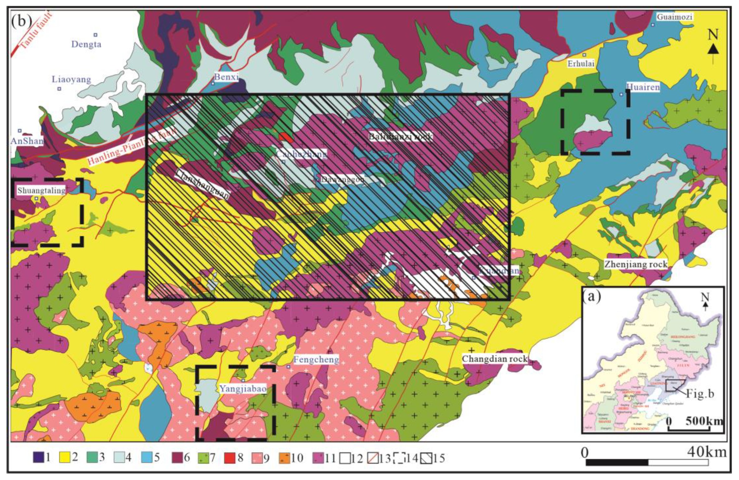
3.2.1. Geological Data

Geological data include mineral geological maps and borehole histograms. The stratigraphic units and occurrences in the mineral geological map are used as input data. Stratigraphic units are encoded in one-hot. For example, the stratigraphic sequence developed in a region from top to bottom might be Gaixian (Pt₁gx), Dashiqiao (Pt₁d), Gaojiayu (Pt₁g), Lieryu (Pt₁lr), and Langzishan (Pt₁l). When the exposed stratum on the surface is the Dashiqiao formation, the input stratigraphic unit code is 01000. The occurrence of the stratigraphic unit only considers the dip angle during input, and the dip angle is expressed in radians. Borehole histograms are used for stratum constraints and are encoded in the same way as the stratigraphic unit. If the area has no borehole data, the channel datum is set to 0 for processing.

3.2.2. Geophysical Data

Generally, gravity and aeromagnetic anomaly data are the common geophysical data. Geological surveys and geophysical exploration have been carried out in the area where 3D geological modeling is to be performed. A number of geophysical sections can be collected, or a certain number of geophysical comprehensive interpretation sections can be compiled on the basis of the measured data. These sections should reflect various underground geological conditions in a region. These geophysical data cannot be used in the networks, unless a data gridding operation is performed.

3.2.3. Data Gridding

In order to grid the geophysical data, an interpolation algorithm is needed. In the geology filed, Kriging interpolation is the most used algorithm. According to the sparse degree of the geophysical data and the scale of the study area, a grid size needs to be determined. For example, in the 1:250,000 area, a 300 m × 300 m grid interval can meet the needs of geological research. After interpolation, the geophysical data are transformed into regular data.

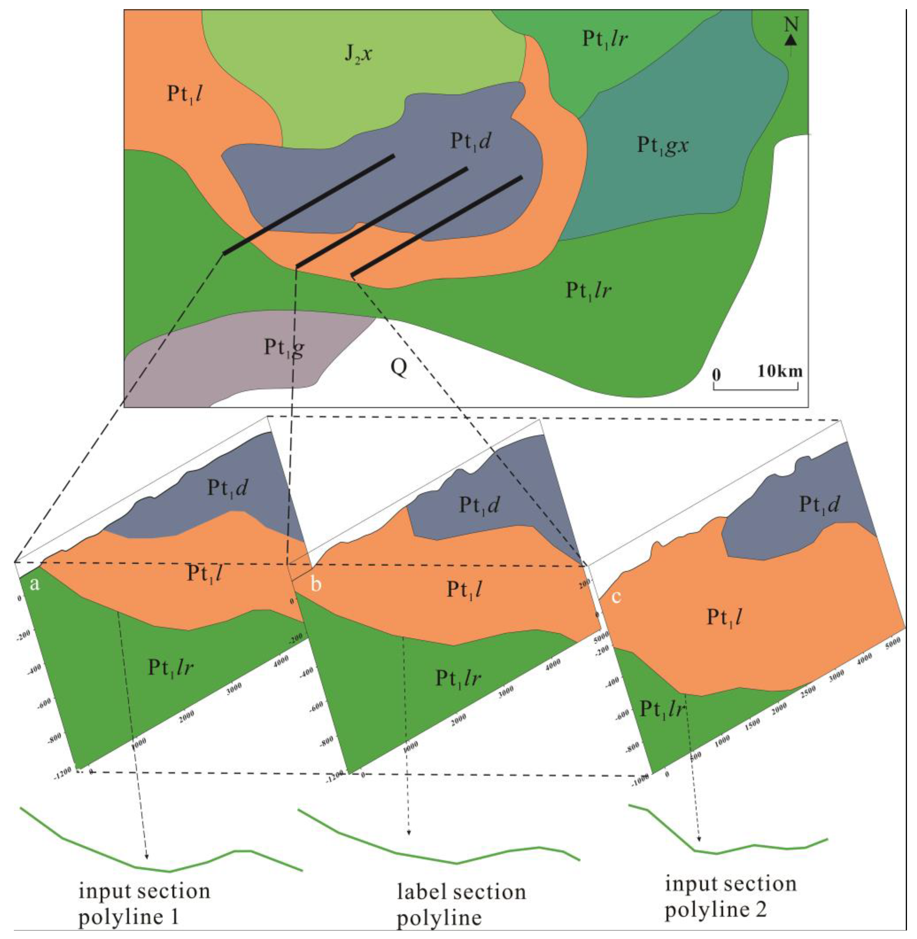
3.2.4. Construction of the Input Dataset

We assume that the data vectors of two adjacent sections are a₁ and a₂. The gravity anomaly data corresponding to these two sections are g₁ and g₂. Anomaly data from the aeromagnetic method are denoted by m₁ and m₂. The sections a₁ and a₂ contain multiple section polylines, set as al_1i and al_2j, i 1, 2, …, n, j ∈ 1, 2, …, m. According to the stratigraphic age of the polyline in the section, we take section polylines with the same stratigraphic age P, that is, P_1i==P_2j, to form a section polyline pair (al_1i, al_2j) from top to bottom. When there is a pinch out, the missing section polyline datum is set to 0.

Every section polyline pair (al_1i, al_2j) is interpolated to form 256 points, and then each section polyline is copied 256 times to form a 256 × 256 matrix, recorded as AL_1i and AL_2j.

Then, the same operation is applied to g₁, g₂, m₁ and m₂, and a channel of a 256 × 256 matrix is formed, marked as G₁, G₂, M₁ and M₂.

While generating the modeling section with the input sections of a₁ and a₂, the distance between the generated section and the two input sections will also affect the shape of the section polylines in the modeling. Therefore, this method introduces the distance factor d as a parameter.

$$\{\begin{array}{c}d=\frac{d_1}{d_2}\\ d_1=\sqrt{{(p_{1x}-p_{mx})}^2+{(p_{1y}-p_{my})}^2}\\ d_2=\sqrt{{(p_{1x}-p_{2x})}^2+{(p_{1y}-p_{2y})}^2}\end{array}$$

(5)

The parameter d is calculated as follows (Equation (5)).

The middle points p₁ of section a₁ and p₂ of section a₂ are calculated.

Points p₁ and p₂ are connected, where upon the line p₁p₂ intersects the generated section a_m at p_m.

Length d₁ of p₁p_m and length d₂ of p₁p₂ are calculated.

It is assumed that d = d₁/d₂.

A 256 × 256 matrix D is filled with the value of d as an input channel.

For the interpolated section, once the section line a_m (see Figure 5) is determined, the gravity data g_m corresponding to the section line and aeromagnetic data m_m are known. After the interpolation of gravity and aeromagnetic data formed as a 2 × 256 matrix, the matrix is padded to form a 256 × 256 matrix, marked as G_m and M_m, where m × 1, 2, …, 256. Therefore, G_m, M_m and the previously generated AL_1i, AL_2j, G₁, G₂, M₁ M₂ and D are stacked as input matrices with the shape of 256 × 256 × 9 and recorded as input.

3.2.5. Label Data

In the training stage, a label is required. Different with the classification model, the generation model needs section data as a label. Similar to the preparation process of input data, the section polyline al_mi, corresponding to stratigraphic age in section a_m, is interpolated into 256 points, then padded into a 256 × 256 matrix forming the label data and marked as label.

3.3. Data Augmentation

Since each section contains multiple section polylines, and the data used for training in this method is a single section polyline, polylines of the section map can be extracted as training data (see Figure 6), thus enhancing the data volume and avoiding overfitting.

Figure 6 shows the method of data augment in this study. In each section, the interface of two different geological bodies decides the top or the bottom. So, section polylines are the objects of this method. Every interface in the section is used for the training process, thus augmenting the dataset.

4. Results and Discussion

To verify the generating ability of the proposed method, we conducted experiments in the Benxi–Huanren area in eastern Liaoning Province, China (see Figure 7). This area has been surveyed by certain geological survey projects. The geological, gravity and aeromagnetic data are available.

In this section, the data of training is described firstly, and then the environment of the experiment is listed. Finally, the results are discussed.

4.1. Data and Data Processing

In the study area, we collected 1650 section pairs, including 467 simple stratum sections, 332 complex stratum sections, 420 rock mass sections and 431 fault sections (see

Table 1. The amount of collected data for training.

Type	Section Pairs	Samples
Simple strata	467	4281
Complex strata	332	1672
Rock masses	420	420
Faults	431	431
Total	1650	6804

) in the location of dataset area (see Figure 7). According to the data augment method, the section polylines are extracted from the section pairs. Finally, 6804 samples are prepared. Correspondently, the gravity data, aeromagnetic data, and other data for the 6804 samples are calculated with the instruction of Section 3.2.

In order to evaluate the proposed method, we divided the samples into training, validating and testing datasets with the proportion of 8:2. Here, 20% of the training dataset are used for validation during the training process. Thus, 5443 samples are used for training, 1088 samples of the training dataset are used for validating, and 1361 samples are used for testing.

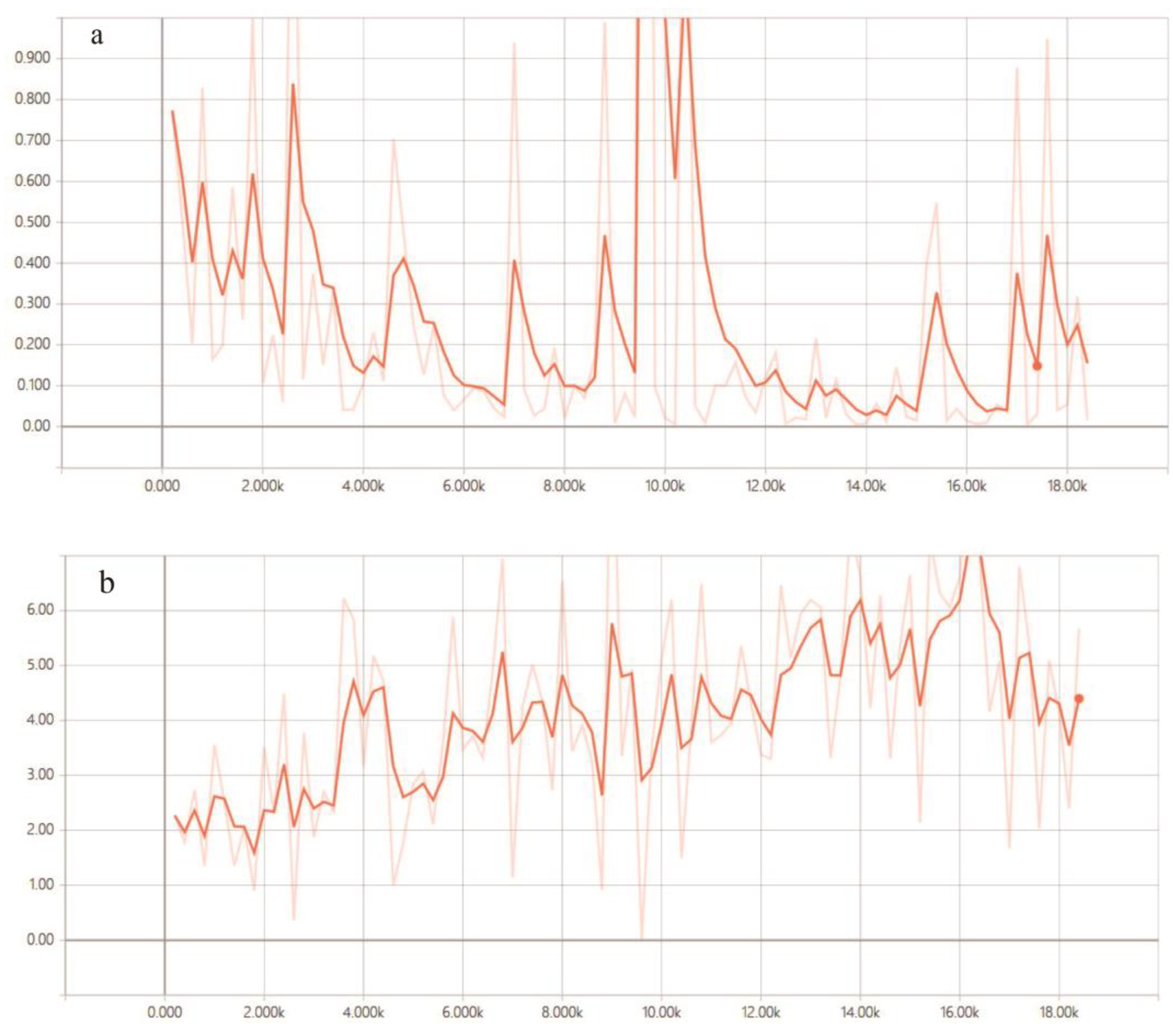
4.2. Experiments and Results

In order to quantify the difference between the generated section and the real section, this study used the arithmetic mean deviation of section (AMDoS, Equation (6)) as the evaluation standard, where (x_i, y_i) is the coordinates of the ith point on the label section polyline, and (x_i’, y_i’) are the coordinates of the ith point in the generated section polyline.

$$AMDoS={\displaystyle {\sum }_{i=1}^{11}(\sqrt{{(x_i-x_i^{\prime })}^2+{(y_i-y_i^{\prime })}^2}}$$

(6)

Since the number of points in the real section is inconsistent with the number of points in the generated section, when calculating the error value, we calculate the length of the curve, divide the curve into 10 equal parts on average from the starting point of the curve, and calculate the end point of each curve as the error calculation point, including the starting point of the overall curve for 11 points (Equation (6)).

Simultaneously, the coincidence rate of point coordinates (CRoPC, Equation (7)) is calculated, where TP is the point number with the deviation being less than AMDoS, and on the other hand, FP is the deviation more than AMDoS.

$$CR\mathrm{o}PC=\frac{TP}{TP+FP}$$

(7)

If the CRoPC value is more than 0.5, the generated section polyline is considered a positive sample, otherwise a negative sample. So, with this method, we can obtain an accuracy of the proposed model.

The experiments described here run on a computer with the configuration listed in

Table 2. Hardware and software configurations used in the experiment.

Configuration	Value
CPU	Intel Core i5-7300HQ 2.5 GHz
GPU	NVIDIA GeForce GTX 1050Ti with 4GB RAM
Memory	8 GB
Hard disk	1 TB
Operating System	Windows 10
Python Version	3.6.5
Tensorflow Version	Tensorflow-GPU 1.5.0

.

Different super parameters, such as epochs, initial learning rate (ILR), decay rate and batch size, play an important role in the learning effect. Therefore, it is necessary to test the impact of different super parameters on the generator to obtain a relative optimal solution (see Discussion for specific experiments). Finally, with an initial learning rate of 10⁻⁴, two samples in a batch, 10⁻³ decay of learning rate, the model ran 18,000 epochs of training and validating, and achieved a validating accuracy of 92%. The correspondent curves of cross-entropy losses are shown in Figure 8.

Figure 8 shows that at the beginning of training, the loss curve of the discriminator fluctuated, indicating that the training parameters were being adjusted frequently and that this had a significant impact on the generator. When the number of training steps reached 6000, the loss of the discriminator decreased steadily. After a large shock with 10,000 training steps, the loss value of the D dropped to the lowest point after 14,000 steps, and the loss curve of G was relatively stable at this time. Then, the curves of the generator and discriminator began to fluctuate again. Therefore, the trained model after 14,000 steps can be taken for generating modeling sections.

Part of the cross sections generated by the trained CGAN model are shown in Figure 9. It can be seen from the comparison of label section polylines that those generated using the proposed method (Figure 9b,d) are smoother than the label section polylines (Figure 9a,c).

4.3. Influence of Different Super Parameters on the Results

The super parameters affect the performance and accuracy of the proposed model.

Table 3. Performance on different super parameter settings of the proposed method.

Experiments	Epochs	ILR	Batch	Decay	Validation Accuracy
1	18,000	10−3	2	10−3	86%
2	18,000	10−3	2	10−4	87.2%
3	18,000	10−3	2	10−5	85%
4	18,000	10−4	2	10−3	92%
5	18,000	10−4	2	10−4	88%
6	18,000	10−4	2	10−5	89%
7	18,000	10−5	2	10−3	91%
8	18,000	10−5	2	10−4	86%
9	18,000	10−5	2	10−5	85%

compares the accuracy when using different super parameter settings to train the model.

The experimental results show that different super parameters will exhibit different validation accuracies. Due to the limits of the configuration of the executing computer, the batch size is set to 2, and in consideration of the run time, the epoch value is set to 18,000. When the ILR is 10⁻⁴, and decay is 10⁻³, the proposed model achieved an overall accuracy of 92%.

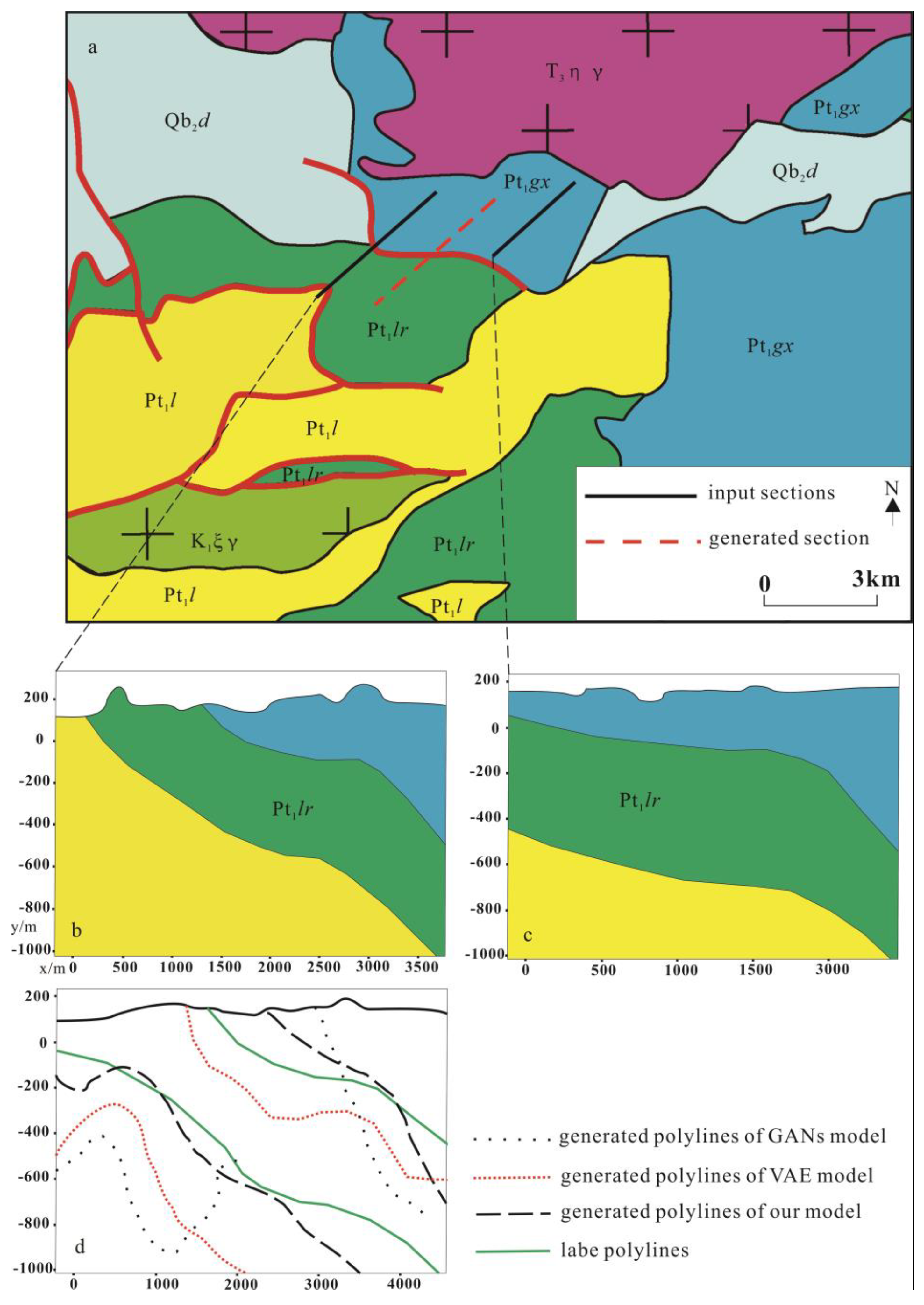
4.4. Comparison with Other Deep Learning Algorithms

In order to test the superiority of the proposed method, the VAE model and the common GAN model are also used for generating cross sections, and the sections generated by the three models are compared (see Figure 10).

AutoEncoder is a generative model [25]. It is suitable for image editing using concept vectors. It maps the input data to a potential vector space through an encoder module, and then decodes it to an output with the same size as the original input through a decoder.

By adding statistical operations to the AutoEncoder network, VAE [44] enables the AutoEncoder network to learn a continuous and highly structured potential space, thus becoming a powerful tool in the field of image generation. The traditional VAE includes two parts: the encoder and decoder. The encoder module is used to collect and train the features of the input data and generate the feature distribution of the training data, and then the decoder module is used to generate the section data to be interpolated based on the feature distribution.

The encoder module is implemented through a convolution operation. After three consecutive convolution operations, a dropout operation is added to discard some data, improve the generalization ability of the model, and finally produce a full connection layer as the output of the encoder module.

The decoder module was created through a four-layer deconvolution operation. Through the deconvolution operation, the potential feature space data extracted by the encoder module is dimensionally restored to finally achieve the purpose of generating the data.

Using the same training and validating dataset, we trained the VAE and GAN models. The statistics of AMDoS, CRoPC and validation accuracy are calculated (see

Table 4. Effect evaluation of different models.

Methods	VAE	GAN	Our Work
Max AMDoS	1568.49	3351.65	1021.61
Min AMDoS	352.84	2015.68	154.23
Max CRoPC	83%	65%	92%
Min CRoPC	37%	32%	44%
Validation accuracy	68%	45%	87%

). A generated section by the three models is compared (see Figure 10).

Table 4 gives the statistical information of the three models’ training processes. The AMDoS value and CRoPC are quite different with the VAE, GAN and our model. The deviations of the GAN model are bigger than those of the other two models. Consequently, the GAN model has the worst performance and 45% validation accuracy. In contrast, our work performs well, both in the deviation value and the validation accuracy of 87%, and the VAE model performs better than the GAN model, but worse than our work.

It can be seen from Figure 10 that the section generated by the GAN model is quite different from the labeled section, seriously deviating from the label. The polylines generated by the VAE and our model are consistent with the label.

5. 3D Geological Modeling and Application

After the training is completed, the network parameters are frozen. Three different application tests (see Figure 7), Yangjiabao, Shuangtaling and Huanren, are carried out in the study area.

The geological, gravity and aeromagnetic data, and few main sections [13] of the test areas are provided. Using the frozen network parameters, cross sections are generated every 50 m from left to right in the test areas, and finally 29 horizontal cross sections in each test area are obtained. Similarly, 24 vertical cross sections in each test area are obtained from top to bottom. The 3D geological models are established on the basis of the generated sections using the modeling method based on cross sections (see Figure 11).

The test results show that, the 3D geological models as illustrated in Figure 11 basically conforms to the geological principles of the study areas, and the model is relatively smooth. Compared with the Yangjiabao area, the geology of the Huanren and Shuangtaling areas are more complex, with structures such fold and fault growing in these two areas. These 3D models also prove that the proposed method can generate section data intelligently, with good stability and practicality.

6. Conclusions

In this study, we considered the key problem of inefficiency of drawing cross sections, and an intelligent method for generating cross sections based on the CGAN model using multi-source and heterogeneous geological data, such as geological, gravity and aeromagnetic anomaly data. After the proposed model was trained, this method achieved an overall accuracy of 87%. Cross sections at the specified location can be generated using the trained model. We tested the method via the establishment of three different 3D geological models in the areas of Yangjiabao, Shuangtaling and Huanren, Liaoning Province. The experimental results show the proposed method can improve the drawing efficiency of the cross sections significantly.

At present, the problem remains that the generated cross sections may not conform to the actual situation when the trained model is used to build a complex section, which has multiple structures and intrusions. To solve this problem, we will try improving the method from two aspects in the following research. First, we can increase the size of the training dataset. The more training data there are, the better the model can update the corresponding model parameters so when applied to new areas, it can generate relatively more accurate sections. Second, the super parameters in the model (such as batch size and the gradient descent algorithm) can be tested to find the optimal network parameters in order to train a more accurate network model.

References

1. Pan, M.; Li, Z.; Gao, Z.; Yang, Y.; Wu, G. 3-D geological modeling-concept, methods and key techniques. Acta Geol. Sin. (Engl. Ed.) 2012, 86, 1031–1036. [Google Scholar]
2. Wang, G.; Li, R.; Carranza, E.J.M.; Zhang, S.; Yan, C.; Zhu, Y.; Qu, J.; Hong, D.; Song, Y.; Han, J.; et al. 3D geological modeling for prediction of subsurface Mo targets in the Luanchuan district, China. Ore Geol. Rev. 2015, 71, 592–610. [Google Scholar] [CrossRef]
3. Wang, G.; Zhu, Y.; Zhang, S.; Yan, C.; Song, Y.; Ma, Z.; Hong, D.; Chen, T. 3D geological modeling based on gravitational and magnetic data inversion in the Luanchuan ore region, Henan Province, China. J. Appl. Geophys. 2012, 80, 1–11. [Google Scholar] [CrossRef]
4. Ming, J.; Pan, M.; Qu, H.; Ge, Z. GSIS: A 3D geological multi-body modeling system from netty cross-sections with topology. Comput. Geosci. 2010, 36, 756–767. [Google Scholar] [CrossRef]
5. Bistacchi, A.; Massironi, M.; Dal Piaz, G.V.; Dal Piaz, G.; Monopoli, B.; Schiavo, A.; Toffolon, G. 3D fold and fault reconstruction with an uncertainty model: An example from an Alpine tunnel case study. Comput. Geosci. 2008, 34, 351–372. [Google Scholar] [CrossRef]
6. Whiteaker, T.L.; Jones, N.; Strassberg, G.; Lemon, A.; Gallup, D. GIS-based data model and tools for creating and managing two-dimensional cross sections. Comput. Geosci. 2012, 39, 42–49. [Google Scholar] [CrossRef]
7. Lemon, A.M.; Jones, N.L. Building solid models from boreholes and user-defined cross-sections. Comput. Geosci. 2003, 29, 547–555. [Google Scholar] [CrossRef]
8. Zhu, L.F.; Wu, X.C.; Liu, X.G.; Shang, J.G. Reconstruction of 3D strata model based on borehole data. Geogr. Geo-Inf. Sci. 2004, 20, 26–30. [Google Scholar]
9. Wu, Q.; Xu, H.; Zou, X. An effective method for 3D geological modeling with multi-source data integration. Comput. Geosci. 2005, 31, 35–43. [Google Scholar] [CrossRef]
10. Ming, J. Quick construction and update of three-dimensional geological models based on boreholes. Geogr. Geo-Inf. Sci. 2012, 28, 55–59, 113. [Google Scholar]
11. Chen, G.L.; Liu, X.G.; Sheng, Q.; Zhang, Y.H. A modeling method based on intersected geological sections. Rock Soil Mech. 2011, 32, 2409–2415. [Google Scholar]
12. Guo, Y.J.; Pan, M.; Wang, Z.; Wang, Y.; Wu, Z.X.; Qu, H.G.; Ming, J. Research on three-dimensional geological modeling method based on drilling data and constraints of intersected folded cross-sections. Geogr. Geo-Inf. Sci. 2009, 25, 23–26. [Google Scholar]
13. Xue, L.F.; Li, W.Q.; Zhang, W.; Chai, S.L.; Liu, Z.H. A method of block-divided 3D geologic modeling in regional scale. J. Jilin Univ. Earth Sci. Ed. 2014, 44, 2051–2058. [Google Scholar]
14. Zhang, W.; Xue, L.F.; Peng, C.; Chai, Y.; Cheng, W. The 3D modeling method based on profiles and its application in Benxi, Liaoning province. Geol. Resour. 2013, 22, 403–408. [Google Scholar]
15. Qu, H.G.; Pan, M.; Ming, J.; Wu, Z.X.; Sun, Z.D. An efficient method for high-precision 3D geological modeling from intersected folded cross-sections. Acta Sci. Nat. Univ. Pekin. 2008, 44, 84–89. [Google Scholar]
16. Pan, M.; Fang, Y.; Qu, H.G. Discussion on several foundational issues in three-dimensional geological modeling. Geogr. Geo-Inf. Sci. 2007, 23, 1–5. [Google Scholar]
17. Wang, G.; Huang, L. 3D geological modeling for mineral resource assessment of the Tongshan Cu deposit, Heilongjiang Province, China. Geosci. Front. 2012, 3, 483–491. [Google Scholar] [CrossRef] [Green Version]
18. Qi, G.; Lv, Q.T.; Yan, J.Y.; Wu, M.A.; Liu, Y. Geologic constrained 3D gravity and magnetic modeling of Nihe deposit-A case study. Chin. J. Geophys. 2012, 55, 4194–4206. [Google Scholar]
19. Jia, R.; Wang, H.R.; Wang, G.W.; Wang, H.; Xu, R.D.; Feng, Z.K.; Song, Y.W.; Wang, X.L.; Pang, Z. Three-dimensional geological modeling and deep prospectivity of the Xigou Pb-Zn-Ag-Au deposit, Henan Province. Earth Sci. Front. 2021, 28, 156–169. [Google Scholar]
20. Wang, G.W.; Zhang, T.S.; Yan, C.H.; Song, Y.W.; Chen, T.Z.; Li, D.; Ma, Z.B. 3D geological modeling based on geological and gravity-magnetic data integration in the Luanchuan Molybdenum Polymetallic deposit, China. Earth Sci. -J. China Univ. Geosci. 2011, 36, 360–366. [Google Scholar]
21. Zhu, L.F.; Pan, X. Reconstruction of 3D stratigraphic model for fluvial erosion and aggrading action. Rock Soil Mech. 2005, 26 (Suppl. S1), 65–68. [Google Scholar]
22. Zhong, D.H.; Li, M.C.; Song, L.G.; Wang, G. Enhanced NURBS modeling and visualization for large 3D geoengineering applications: An example from the Jinping first-level hydropower engineering project, China. Comput. Geosci. 2006, 32, 1270–1282. [Google Scholar] [CrossRef]
23. Ming, J.; Yan, M. Three-dimensional geological surface creation based on morphing. Geogr. Geo-Inf. Sci. 2014, 30, 37–40. [Google Scholar]
24. Wu, Z.C.; Guo, F.S.; Zhang, W.L.; Ying, Y.G.; Zhou, W.P.; Li, C. 3D geological modeling based on multi-source data merging of Xiangshan volcanic basin in Le’an of Jiangxi. J. Guilin Univ. Technol. 2020, 40, 310–322. [Google Scholar]
25. Ackley, D.H.; Hinton, G.E.; Sejnowski, T.J. A learning algorithm for Boltzmann machines. Cogn. Sci. 1985, 9, 147–169. [Google Scholar] [CrossRef]
26. Yang, M.L.; Xue, L.F.; Ran, X.J.; Sang, X.J.; Yan, Q.; Dai, J.H. Intelligent mineral geological survey method: Daqiao-Yawan area in Gansu Province as an example. Acta Petrol. Sin. 2021, 37, 3880–3892. [Google Scholar]
27. Guo, J.; Li, Y.; Jessell, M.W.; Giraud, J.; Li, C.; Wu, L.; Li, F.; Liu, S. 3D geological structure inversion from Noddy-generated magnetic data using deep learning methods. Comput. Geosci. 2021, 149, 104701. [Google Scholar] [CrossRef]
28. Hillier, M.; Wellmann, F.; Brodaric, B.; de Kemp, E.; Schetselaar, E. Three-dimensional structural geological modeling using graph neural networks. Math. Geosci. 2021, 53, 1725–1749. [Google Scholar] [CrossRef]
29. Liu, Q.; Liu, W.; Yao, J.; Liu, Y.; Pan, M. An improved method of reservoir facies modeling based on generative adversarial networks. Energies 2021, 14, 3873. [Google Scholar] [CrossRef]
30. Li, S.; Chen, J.; Liu, C.; Wang, Y. Mineral prospectivity prediction via convolutional neural networks based on geological big data. J. Earth Sci. 2021, 32, 327–347. [Google Scholar] [CrossRef]
31. Guo, M.; Bei, W.; Huang, Y.; Chen, Z.; Zhao, X. Deep learning framework for geological symbol detection on geological maps. Comput. Geosci. 2021, 157, 104943. [Google Scholar] [CrossRef]
32. Tang, M.; Liu, Y.; Durlofsky, L.J. Deep-learning-based surrogate flow modeling and geological parameterization for data assimilation in 3D subsurface flow. Comput. Methods Appl. Mech. Eng. 2020, 376, 113636. [Google Scholar] [CrossRef]
33. Zhang, T.F.; Tilke, P.; Dupont, E.; Zhu, L.; Liang, L.; Bailey, W. Generating geologically realistic 3D reservoir facies models using deep learning of sedimentary architecture with generative adversarial networks. Pet. Sci. 2019, 16, 541–549. [Google Scholar] [CrossRef] [Green Version]
34. Goodfellow, I.; Pouget-Abadie, J.; Mirza, M.; Xu, B.; Warde-Farley, D.; Ozair, S.; Courville, A.; Bengio, Y. Generative adversarial nets. In Proceedings of the Advances in Neural Information Processing Systems, Montreal, QC, Canada, 8–13 December 2014; pp. 2672–2680. [Google Scholar]
35. Krizhevsky, A.; Sutskever, I.; Hinton, G. ImageNet classification with deep convolutional neural networks. In Proceedings of the 25th International Conference on Neural Information Processing Systems, Lake Tahoe, NV, USA, 3–6 December 2012; pp. 1097–1105. [Google Scholar]
36. Simonyan, K.; Zisserman, A. Very deep convolutional networks for large-scale image recognition. arXiv 2014, arXiv:1409.1556. [Google Scholar]
37. Szegedy, C.; Liu, W.; Jia, Y.; Sermanet, P.; Rabinovich, A. Going deeper with convolutions. In Proceedings of the 2015 IEEE Conference on Computer Vision and Pattern Recognition (CVPR 2015), Boston, MA, USA, 8–10 June 2015; pp. 1–9. [Google Scholar]
38. Mirza, M.; Osindero, S. Conditional Generative Adversarial Nets. arXiv 2014, arXiv:1411.1784. [Google Scholar]
39. Ferreira, A.; Giraldi, G. Convolutional neural network approaches to granite tiles classification. Expert Syst. Appl. 2017, 84, 1–11. [Google Scholar] [CrossRef]
40. Liu, B.; Zhang, Y.; He, D.; Li, Y. Identification of apple leaf diseases based on deep convolutional neural networks. Symmetry 2017, 10, 11. [Google Scholar] [CrossRef] [Green Version]
41. Ran, X.J.; Xue, L.F.; Zhang, Y.Y.; Liu, Z.Y.; Sang, X.J.; He, J.X. Rock classification from field image patches analyzed using a deep convolutional neural network. Mathematics 2019, 7, 755. [Google Scholar] [CrossRef]
42. Zhang, Y.Y.; Ran, X.J. A step-based deep learning approach for network intrusion detection. Comput. Model. Eng. Sci. 2021, 128, 1231–1245. [Google Scholar] [CrossRef]
43. Peng, C.; Xue, L.F.; Liu, Z.H.; Liu, H.Y. Application of the Non-seismic Geophysical method in the Deep Geological Structure Study of Benxi-Huanren Area. Arab. J. Geosci. 2016, 9, 1–15. [Google Scholar] [CrossRef]
44. Diederik, P.K.; Max, W. Auto-Encoding Variational Bayes. arXiv 2013, arXiv:1312.6114. [Google Scholar]
Figure 1. Flow chart of the GAN model.
Mathematics 10 04677 g001
Figure 2. CGAN network structure.
Mathematics 10 04677 g002
Figure 3. The operation of the convolution layer.
Mathematics 10 04677 g003
Figure 4. Intelligent generating model for cross sections. I: Geological coding data. II: Gravity anomaly and continuation data. III: Aeromagnetic anomaly and continuation data. IV: Points of the known section polyline. V: Distance coefficient. VI: Points of generated section polyline.
Mathematics 10 04677 g004
Figure 5. Section interpolation and parameters diagram.
Mathematics 10 04677 g005
Figure 6. Examples of training dataset. (a) input Section 1; (b) label section; (c) input Section 2.
Mathematics 10 04677 g006
Figure 7. Simplified geological map of the study area (after the 1:500,000 geological map produced by the Geological Survey of China, modified from [43]). 1. Archean. 2. Paleoproterozoic. 3. Mesoproterozoic- Neoproterozoic. 4. Paleozoic. 5. Mesozoic. 6. Archean granitic gneiss. 7. Paleoproterozoic granite. 8. Early Triassic basic-ultrabasic complex. 9. Triassic granite. 10. Late Triassic granite. 11. Yanshanian granite. 12. Other geological units. 13. Fault. 14. Location of test area. 15. Location of dataset. (a) The Benxi–Huanren area in eastern Liaoning Province, China; (b) the close-up of the area in (a).
Mathematics 10 04677 g007
Figure 8. Loss curves during CGAN training. (a) Discriminator D loss curve; (b) generator G loss curve.
Mathematics 10 04677 g008
Figure 9. Comparison between the label and the generated section polyline in our work. (a) Label of complex stratum; (b) generated section polyline of complex stratum; (c) label of rock mass; (d) generated section polyline of rock mass.
Mathematics 10 04677 g009
Figure 10. Comparison with the model of VAE, GANs and our work. (a) Geological background of the selected result; (b,c) input sections; (d) comparison of the sections generated by the three models and label.
Mathematics 10 04677 g010
Figure 11. 3D geological models built from the generated sections. (a) Huanren area; (b) Shuangtaling area; (c) Yangjiabao area.
Mathematics 10 04677 g011