Article

Adaptive Fuzzy Command Filtered Finite-Time Tracking Control for Uncertain Nonlinear Multi-Agent Systems with Unknown Input Saturation and Unknown Control Directions

1
Key Laboratory of Electric Drive and Control of Anhui Higher Education Institutes, Anhui Polytechnic University, Wuhu 241000, China
2
Key Laboratory of Advanced Perception and Intelligent Control of High-End Equipment, Ministry of Education, Anhui Polytechnic University, Wuhu 241000, China
*
Author to whom correspondence should be addressed.
Mathematics 2022, 10(24), 4656; https://doi.org/10.3390/math10244656
Submission received: 16 November 2022 / Revised: 3 December 2022 / Accepted: 6 December 2022 / Published: 8 December 2022
(This article belongs to the Topic Dynamical Systems: Theory and Applications)

Abstract

:
This paper investigates the finite-time consensus tracking control problem of uncertain nonlinear multi-agent systems with unknown input saturation and unknown control directions. An adaptive fuzzy finite-time consensus control law is proposed by combining the fuzzy logic system, command filter, and finite-time control theory. Using the fuzzy logic systems, the uncertain nonlinear dynamics are approximated. Considering the command filter and backstepping control technique, the problem of the so-called “explosion of complexity” in the design of virtual control laws and adaptive updating laws is avoided. Meanwhile, the Nussbaum gain function method is applied to handle the unknown control directions and unknown input saturation problems. Based on the finite-time control theory and Lyapunov stability theory, it was found that all signals in the closed-loop system remained semi-global practical finite-time stable, and the tracking error could converge to a sufficiently small neighborhood of the origin in the finite time. In the end, simulation results were provided to verify the validity of the designed control law.

1. Introduction

The consensus problem for multi-agent systems has been widely investigated over the past few decades due to its applications in aircraft formation control [1], autonomous unmanned systems [2], wireless sensor networks [3], and other fields. Many remarkable research findings, such as the adaptive cooperative control of nonlinear multi-agent systems [4], adaptive distributed control of non-affine multi-agent systems [5], iterative learning control of nonlinear multi-agent systems [6], distributed optimization control of linear multi-agent systems [7,8], adaptive event-triggered control of multi-agent systems [9,10], and so on, have been extensively reported. It is not difficult to find that in many existing achievements on multi-agent systems, the fuzzy logic system and neural network approach have been successfully applied to approximate the unknown nonlinear dynamics by many researchers; see [11,12,13,14] and references therein. Meanwhile, to obtain the final control law, the backstepping control technique and dynamic surface control technique have been considered by researchers [15,16]. Moreover, in [17,18], an improved command filter control method is addressed, where the compensating signal that does not need to take the derivative of the filtering error is applied, and the so-called “explosion of complexity” problem caused by the traditional backstepping control method is solved. However, it should be noted that in many practical systems, the control directions of these systems may not be known a priori or may be affected by actuator faults. Therefore, it is of more practical significance to consider these cases.
For the issue of control direction, the sign of control gain may not always be known when considering the existence of unmeasurable state variables and unknown uncertainties. Fortunately, the Nussbaum gain function method is presented and is usually used to deal with the unknown control direction, which was first reported in [19]. Subsequently, the method has been widely utilized for the adaptive control problems of kinds of systems under unknown control directions [20,21,22], to name only a few. More recently, the unknown control direction problems for multi-agent systems have been discussed in many references. In [23], the authors studied a class of multi-agent systems with second-order nonlinear dynamics, where the unknown control directions and position constraints are simultaneously considered and the designed position-constrained consensus control law ensured that the consensus errors could converge to zero. In [24,25], high-order nonlinear multi-agent systems with unknown control directions were investigated, where the output-constrained control law and distributed consensus control law have been presented, respectively. Furthermore, the leaderless consensus control for a class of nonlinear multi-agent systems with unknown control directions and strict-feedback form was developed in [26,27], where the designed adaptive control laws ensured that the error surfaces remained bounded and asymptotically converged to zero. However, it should be pointed out that the finite-time control problem was rarely discussed in the above results. Actually, in practical engineering, such as in the chemical reaction process and spacecraft attitude control, it is usually required to achieve stability quickly. Hence, in these cases, finite-time control should be considered. The finite-time control ensures that the tracking errors converge to the desired range within a given settling time. In addition, for the control problem of multi-agent systems with unknown control directions, how to design a finite-time control strategy is a topic worthy of research.
Another issue that needs attention is the faults of control systems, such as input/output saturation, dead-zone, and hysteresis, which are inevitable owing to the influence of external interferences or human factors. Among them, the fault of input saturation exists widely, and many control strategies have been proposed [28,29,30]. In recent years, the consensus control of multi-agent systems with input saturation has attracted the attention of some researchers. Considering the input saturation and unknown leader input, a distributed observer-based output feedback controller for multi-agent systems with multiple leaders was designed in [31]. For a class of singular multi-agent systems with input saturation, the control laws were presented by the authors to solve the semi-global bipartite consensus tracking control problem, where the local information of agents was considered [32]. In [33], an adaptive fuzzy consensus control law for the prescribed performance problem of a type of non-affine stochastic nonlinear multi-agent systems was proposed, where input hysteresis, input saturation, and non-affine nonlinear forms were simultaneously considered. Moreover, in [34,35], the command filter control problem of high-order nonlinear multi-agent systems with input saturation was discussed by the authors, where the problems of bipartite output consensus tracking control and event-triggered adaptive control were solved, respectively. Through the above analysis, it is not difficult to see that the control problems of multi-agent systems with input saturation have been deeply studied. However, it is also easy to see that there are only a few works that have further discussed the coexistence of an unknown control direction and input saturation in the finite-time control problem of multi-agent systems.
Based on the aforementioned discussion, this paper investigates an adaptive fuzzy finite-time consensus control law for nonlinear multi-agent systems with unknown input saturation and unknown control directions. Compared with the existing results, we have the following three main contributions:
(i) A class of nonlinear multi-agent systems is addressed in this paper, where uncertain dynamics, unknown control directions, and unknown input saturation are simultaneously considered, and only the local information of the agents is used. Different from the constant control gains considered in [22,25,27], the control gain considered in this paper is time-varying and the control input of multi-agent systems is subject to saturation constraints.
(ii) An improved command filter is designed, and then an adaptive fuzzy finite-time consensus control law is proposed by using the fuzzy logic system and finite-time control theory. Compared with [16,24,36], in this paper, the derivative of filtering errors generated in recursive design is avoided by introducing filtering compensating signals.
(iii) Based on the Nussbaum gain function method, the problems of unknown control directions and unknown input saturation are effectively solved. It can be seen that the presented control law ensures that all signals in the closed-loop system maintain semi-global practical finite-time stable, and the tracking errors can converge to a sufficiently small neighborhood of the origin in finite time.
The remainder of this paper is arranged as follows. The problem statement and mathematical preliminaries are introduced in Section 2. The design and theoretical analysis of the adaptive finite-time control law is presented in Section 3. Thereafter, Section 4 gives the simulation results, and brief conclusions are shown in Section 5.

2. Problem Statement and Mathematical Preliminaries

In this section, the problem statement and mathematical preliminaries that are used in this paper are provided.

2.1. Problem Statement

Consider a type of uncertain nonlinear multi-agent systems with one leader agent and N follower agents. The dynamic model of the i th agent is given as
x ˙ i , m = x i , m + 1 + f i , m ( x ¯ i , m ) + γ i , m T φ i , m ( x ¯ i , m ) ,   m = 1 , , n 1 x ˙ i , n = g i ( t ) u i F ( t ) + f i , n ( x ¯ i , n ) + γ i , n T φ i , n ( x ¯ i , n ) y i = x i , 1
where i = 1 , , N , x ¯ i , m = [ x i , 1 , , x i , m ] T R m and x ¯ i , n = [ x i , 1 , , x i , n ] T R n are the state vectors; u i F ( t ) R and y i R are the control input and output of the i th follower agent, respectively; φ i , m ( x ¯ i , m ) and φ i , n ( x ¯ i , n ) are known smooth continuous nonlinear function; f i , m ( x ¯ i , m ) and f i , n ( x ¯ i , n ) , γ i , m and γ i , n are unknown smooth nonlinear functions and unknown parameter vectors, respectively; g i ( t ) is an unknown time-varying nonlinear function representing the direction of the control input and g i ( t ) 0 . Here, the system input u i F ( t ) suffers from saturation nonlinearity, which is described as
u i F ( t ) = s a t ( u i ( t ) ) = { u i , max ,   u i ( t ) u i , max u i ( t ) ,   u i , min < u i ( t ) < u i , max u i , min ,   u i ( t ) u i , min
where u i , min < 0 and u i , max > 0 are the unknown saturation boundaries, and u i ( t ) is the actual control input to be designed. Similar to the method proposed in [36], the piecewise smooth function is introduced to process the saturation function and defined as
ρ i ( u i ( t ) ) = { u i , max tanh ( u i ( t ) u i , max ) u i , min tanh ( u i ( t ) u i , min ) = { u i , max e u i ( t ) / u i , max e u i ( t ) / u i , max e u i ( t ) / u i , max + e u i ( t ) / u i , max ,   u i ( t ) 0 u i , min e u i ( t ) / u i , min e u i ( t ) / u i , min e u i ( t ) / u i , min + e u i ( t ) / u i , min ,   u i ( t ) < 0
Hence, u i F ( t ) in (2) is expressed as
u i F ( t ) = ρ i ( u i ) + d i ( u i )
where d i ( u i ) = u i F ( t ) ρ i ( u i ) is a bounded function and satisfies
| d i ( u i ) | = | u i F ( t ) ρ i ( u i ) | max { u i , max ( 1 tanh ( 1 ) ) , u i , min ( tanh ( 1 ) 1 ) } = D i
Based on the application of the median value theorem [37], there exists a constant ƛ , 0 < ƛ < 1 , such that
ρ i ( u i ) = ρ i , u ƛ ( u i u 0 ) + ρ i ( u 0 )
where ρ i , u ƛ = ( ρ i ( u i ) / u i ) | u i = u ƛ and u ƛ = ƛ u i ( t ) + ( 1 ƛ ) u 0 . By selecting u 0 = 0 , one obtains
u i F ( t ) = ρ i , u ι u i ( t ) + d i ( u i )
Moreover, the graph theory is introduced to represent the relationship of information changes among agents. Let G = ( V , E , A ) be a directed graph with N nodes, in which V = { v 1 , , v N } is the set of vertices, = { ( i , j ) ,   i , j V ,   and   i j } is the set of edges, and A = [ a i j ] R N × N is the weighted adjacency matrix of G , respectively. If there is an edge between node i and j , then a i j = a j i 0 and otherwise a i j = a j i = 0 . The set of neighbors of node i is denoted by J i = { v j :   ( v j ,   v i ) } . The Laplacian matrix of G is denoted by L = D A , where D = diag { d 1 , , d N } with d i = j = 1 J i a i j . Graph G is connected if a path exists between any two vertices.
An extended graph is defined as G ¯ = ( V ¯ , E ¯ ) , which is associated with the leader agent and follower agents. Let the leader adjacency matrix as B = diag b 1 , , b N , and if the follower agent i obtains the information of leader agent, then b i = 1 and otherwise b i = 0 .
The control goal is to design an adaptive fuzzy finite-time control law u i ( t ) for the system (1), such that: (i) in the presence of unknown control directions and input saturation, all signals of the closed-loop systems are semi-global practical finite-time stable (SGPFS), and (ii) the output of each follower agent can be synchronized to the leader agent’s output y d .
To achieve the control objective, the following assumptions are given and will be utilized in the subsequent analysis.
Assumption 1.
The directed graph  G ¯  contains a spanning tree and the leader node is the root node.
Assumption 2.
The unknown nonlinear function  g i ( t ) , i = 1 , , N  in system (1) is bounded. That is,  0 < g m | g i ( t ) | g M , where  g m  and  g M  are unknown positive constants.
Remark 1.
Assumption 1 is a basic condition for the directed graph composed of multi-agent systems, which guarantees eigenvalues of  H = L + B  have positive real parts [11,38]. That is to say, each follower agent has at least one neighbor. For Assumption 2, it is usually used to solve the problem of an unknown control direction of the system, see [20,23] and references therein. From the perspective of practical engineering, this assumption is reasonable because the control coefficient of the actual control input  u i ( t )  cannot be infinite in practice.

2.2. Mathematical Preliminaries

To facilitate the design of the consensus control law, we recall several useful preliminaries, including some definitions and lemmas.
Definition 1
[22]. The smooth continuous function  N ( κ )  is called the Nussbaum gain function if the following properties are held
{ lim s sup 1 s 0 s N ( κ ) d κ = + lim s inf 1 s 0 s N ( κ ) d κ =
There are many Nussbaum gain functions such as  κ 2 cos ( κ ) , κ 2 sin ( κ ) , e κ 2 cos ( π κ / 2 ) , e κ 2 sin ( κ ) , and so on. In the following research, the Nussbaum gain function is chosen as  N ( κ ) = κ 2 cos ( κ ) .
Lemma 1
[25]. Let  V ( t )  and  κ ( t )  be smooth functions defined on  [ 0 , t f )  with  V ( t ) 0 , and  N ( κ )  be an Nussbaum gain function. If the following inequality holds
V ( t ) 0 t ( G ( τ ) N ( κ ) + 1 ) κ ˙ d τ + C 0 ,   t [ 0 , t f )
then  V ( t ) , κ ( t ) , and  0 t ( G ( τ ) N ( κ ) + 1 ) κ ˙ d τ  are bounded on  [ 0 , t f ) , where  G ( t )  satisfies  G m | G ( t ) | G M , with  G m  and  G M  being positive constants;  C 0  is the positive constant.
Lemma 2
[39]. Consider the nonlinear system  σ ˙ = f ( σ ) , if scalars  a 1 > 0 ,  a 2 > 0 , and  0 < μ < 1  exist, and a smooth positive definite function  V ( σ )  such that  V ˙ ( σ ) a 1 V μ ( σ ) + a 2 ,   t 0 , then the nonlinear system  σ ˙ = f ( σ )  is SGPFS, and  V ( σ )  satisfies
V μ ( σ ) a 2 ( 1 ϱ ) a 1 ,   t T r
T r = 1 ( 1 μ ) ϱ a 1 [ V 1 μ ( σ ( 0 ) ) ( a 2 ( 1 ϱ ) a 1 ) 1 μ μ ]
where  0 < ϱ < 1 ,  σ ( 0 )  is the initial value of the system.
Lemma 3
[39]. For any real variables,  x  and  y , and any positive constants,  p 1 , p 2 , and p 3 , the following inequality holds
| x | p 1 | y | p 2 p 1 p 1 + p 2 p 3 | x | p 1 + p 2 + p 2 p 1 + p 2 p 3 p 1 p 2 | y | p 1 + p 2
Lemma 4
[39]. For  α k R ,  k = 1 , , n , and  0 < p < 1 , the following relation holds
( k = 1 n | α k | ) p k = 1 n | α k | p n 1 p ( k = 1 n | α k | ) p
Lemma 5
[4]. For any  b R  and  ϑ > 0 , the hyperbolic tangent function satisfies  0 < | b | b tanh ( b / ϑ ) 0.2785 ϑ .

2.3. Fuzzy Logic Systems

In the subsequent analysis, some unknown continuous functions will be approximated by the fuzzy logic systems. A fuzzy logic system usually consists of four parts, that is, the fuzzifier, the fuzzy rule base, the fuzzy inference engine, and the defuzzifier [33,40]. The fuzzy rule base is composed of “if-then” rules of the following form.
R l :   if   x 1   is   F 1 l ,   ,   and   x n   is   F n l ,   then   h   is   G l ,   l = 1 , 2 , , M .
where x = [ x 1 , , x n ] T and h are the fuzzy logic system’s input and output, respectively; M is the total number of “if-then” rules; F 1 l , , F n l and G l are fuzzy sets for linguistic variables x 1 , , x n and h , respectively. By utilizing the singleton function, center average defuzzification, and product inference [33], the fuzzy logic system can be formulated as
h ( x ) = l = 1 M h ¯ l Π i = 1 n μ F i l ( x i ) l = 1 M [ Π i = 1 n μ F i l ( x i ) ]
where h ¯ l = max h R μ G l ( h ) .
Let θ T = [ h ¯ 1 , , h ¯ M ] = [ θ 1 , , θ M ] and ψ ( x ) = [ ψ 1 ( x ) , , ψ M ( x ) ] T , then (14) is rewritten as
h ( x ) = θ T ψ ( x )
where ψ l ( x ) = ( Π i = 1 n μ F i l ( x i ) ) / ( l = 1 M [ Π i = 1 n μ F i l ( x i ) ] ) , l = 1 , 2 , , M .
Lemma 6
[33]. For any continuous function  f ( x )  defined on a compact set  Ω  and any given positive constant  ε , a fuzzy logic system  f * ( x ) = θ * T ψ ( x )  exists in the form of (15), such that
sup x Ω | f * ( x ) f ( θ , ψ ) | ε
where  θ *  is the ideal parameter vector,  ε  is the approximation accuracy and can be arbitrarily small.

3. Main Results and Stability Analysis

In this section, the adaptive fuzzy finite-time consensus control law is designed for controlling the multi-agent systems (1) based on the fuzzy logic system, command filter, finite-time control theory, and Nussbaum gain function method. The design procedure is divided into n steps. At the m th step for the follower agent i , m = 1 , , n 1 , i = 1 , , N , the virtual control law α i , m is designed, and at the n th step, the actual control law u i ( t ) for the follower agent i is proposed.

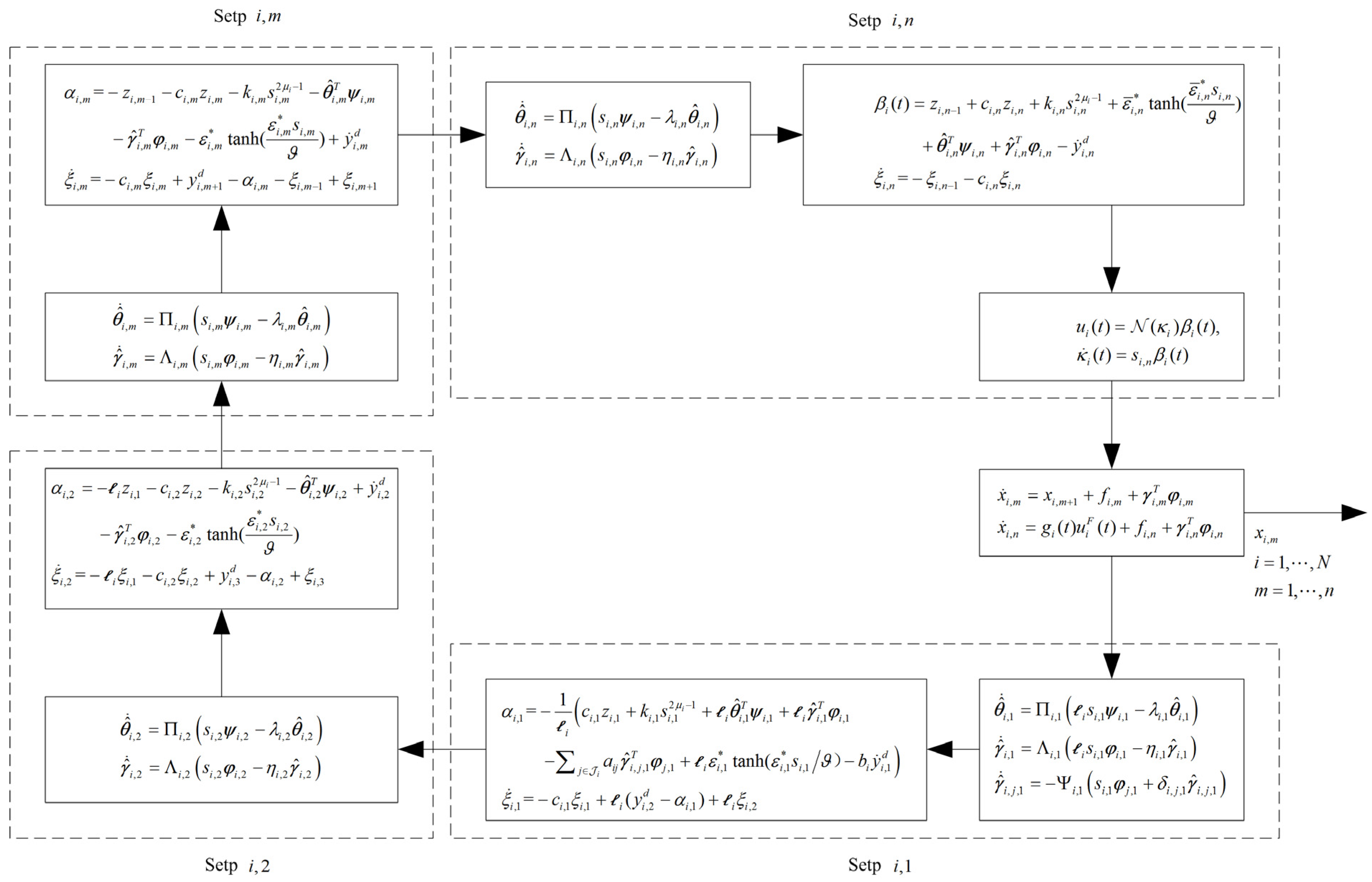
3.1. Adaptive Fuzzy Finite-Time Consensus Control Law Design

The consensus error and coordinate transformation tracking error are given as
z i , 1 = j J i a i j ( y i y j ) + b i ( y i y i , 1 d )
z i , m = x i , m y i , m d ,   m = 2 , , n
where i = 1 , , N and y i , 1 d = y d , y i , m d are the output of a second-order command filter (see Lemma 7) with the virtual control law α i , m 1 as the input.
Lemma 7
[41]. Consider the following second-order command filter with  y i , m d ( 0 ) = α i , m 1 ( 0 )  and ϕ i , m , 2 ( 0 ) = 0  as its initial conditions.
y ˙ i , m d = ω i , m ϕ i , m , 2 ϕ ˙ i , m , 2 = 2 ζ ω i , m ϕ i , m , 2 ω i , m ( y i , m d α i , m 1 )
For any  ν i , m 1 > 0 , constants  ω i , m > 0 ,  m = 2 , , n , and  ζ ( 0 , 1 ]  exist, such that the difference  ( y i , m d α i , m 1 )  is bounded by  ν i , m 1 .
Defining the compensated tracking error s i , m as follows:
s i , m = z i , m ξ i , m
where m = 1 , , n , ξ i , m is the compensating signal to be designed.
Step i , 1 ( 1 i N ): According to (17), (20), and system (1), the derivative of s i , 1 is given as
s ˙ i , 1 = ( j J i a i j + b i ) ( x i , 2 + f i , 1 ( x ¯ i , 1 ) + γ i , 1 T φ i , 1 ( x ¯ i , 1 ) )     j J i a i j ( x j , 2 + f j , 1 ( x ¯ j , 1 ) + γ j , 1 T φ i , 1 ( x ¯ j , 1 ) ) b i y ˙ i , 1 d ξ ˙ i , 1    = i x i , 2 + i F i , 1 + i γ i , 1 T φ i , 1 ( x ¯ i , 1 ) j J i a i j γ j , 1 T φ j , 1 ( x ¯ j , 1 ) b i y ˙ i , 1 d ξ ˙ i , 1
where
i = j J i a i j + b i
F i , 1 = f i , 1 ( x ¯ i , 1 ) 1 i j J i a i j f j , 1 ( x ¯ j , 1 ) 1 i j J i a i j x j , 2
Considering the nonlinear function F i , 1 is unknown, a fuzzy logic system is employed to approximate it, that is,
F i , 1 = θ i , 1 * T ψ i , 1 ( X i , 1 ) + ε i , 1
where X i , 1 = [ x i , 1 , x j , 1 , x j , 2 ] T , ε i , 1 is an approximation error and there exists | ε i , 1 | ε i , 1 * .
Substituting (24) into (21), yields
s ˙ i , 1 = i x i , 2 + i θ i , 1 * T ψ i , 1 ( X i , 1 ) + i ε i , 1 + i γ i , 1 T φ i , 1 ( x ¯ i , 1 ) j J i a i j γ j , 1 T φ j , 1 ( x ¯ j , 1 ) b i y ˙ i , 1 d ξ ˙ i , 1
According to (18), it is obtained that
s ˙ i , 1 = i α i , 1 + i z i , 2 + i ( y i , 2 d α i , 1 ) + i θ i , 1 * T ψ i , 1 ( X i , 1 ) + i ε i , 1 + i γ i , 1 T φ i , 1 ( x ¯ i , 1 )    j J i a i j γ j , 1 T φ j , 1 ( x ¯ j , 1 ) b i y ˙ i , 1 d ξ ˙ i , 1
According to Lyapunov stability theory, and considering estimation errors θ ˜ i , 1 , γ ˜ i , 1 and γ ˜ i , j , 1 , the Lyapunov function candidate V i , 1 in this step is designed as
V i , 1 = 1 2 s i , 1 2 + 1 2 Π i , 1 θ ˜ i , 1 T θ ˜ i , 1 + 1 2 Λ i , 1 γ ˜ i , 1 T γ ˜ i , 1 + 1 2 Ψ i , 1 j J i a i j γ ˜ i , j , 1 T γ ˜ i , j , 1
where θ ˜ i , 1 = θ i , 1 * θ ^ i , 1 , γ ˜ i , 1 = γ i , 1 γ ^ i , 1 and γ ˜ i , j , 1 = γ j , 1 γ ^ i , j , 1 ; Π i , 1 , Λ i , 1 and Ψ i , 1 are positive design constants; θ ^ i , 1 , γ ^ i , 1 and γ ^ i , j , 1 are the estimate of θ i , 1 * , γ i , 1 and γ j , 1 , respectively.
Noting (26), then the derivative of V i , 1 is expressed as
V ˙ i , 1 = s i , 1 s ˙ i , 1 1 Π i , 1 θ ˜ i , 1 T θ ^ ˙ i , 1 1 Λ i , 1 γ ˜ i , 1 T γ ^ ˙ i , 1 1 Ψ i , 1 j J i a i j γ ˜ i , j , 1 T γ ^ ˙ i , j , 1    = s i , 1 ( i α i , 1 + i z i , 2 + i ( y i , 2 d α i , 1 ) + i θ i , 1 * T ψ i , 1 ( X i , 1 ) + i ε i , 1 + i γ i , 1 T φ i , 1 ( x ¯ i , 1 )    j J i a i j γ j , 1 T φ j , 1 ( x ¯ j , 1 ) b i y ˙ i , 1 d ξ ˙ i , 1 ) 1 Π i , 1 θ ˜ i , 1 T θ ^ ˙ i , 1 1 Λ i , 1 γ ˜ i , 1 T γ ^ ˙ i , 1 1 Ψ i , 1 j J i a i j γ ˜ i , j , 1 T γ ^ ˙ i , j , 1
Designing the compensating signal ξ i , 1 as
ξ ˙ i , 1 = c i , 1 ξ i , 1 + i ( y i , 2 d α i , 1 ) + i ξ i , 2
Designing the virtual control law α i , 1 as
α i , 1 = 1 i ( c i , 1 z i , 1 + k i , 1 s i , 1 2 μ i 1 + i θ ^ i , 1 T ψ i , 1 + i γ ^ i , 1 T φ i , 1 j J i a i j γ ^ i , j , 1 T φ j , 1 + i ε i , 1 * tanh ( ε i , 1 * s i , 1 ϑ ) b i y ˙ i , 1 d )
Designing the adaptive laws θ ^ ˙ i , 1 , γ ^ ˙ i , 1 and γ ^ ˙ i , j , 1 as
θ ^ ˙ i , 1 = Π i , 1 ( i s i , 1 ψ i , 1 λ i , 1 θ ^ i , 1 )
γ ^ ˙ i , 1 = Λ i , 1 ( i s i , 1 φ i , 1 η i , 1 γ ^ i , 1 )
γ ^ ˙ i , j , 1 = Ψ i , 1 ( s i , 1 φ j , 1 + δ i , j , 1 γ ^ i , j , 1 )
where μ i ( 0 , 1 ) , c i , 1 , k i , 1 , λ i , 1 , η i , 1 , δ i , j , 1 , and ϑ are the designed constants, respectively.
Considering (20), substituting (29)–(33) into (28), and considering the Lemma 5, yields
V ˙ i , 1 c i , 1 s i , 1 2 k i , 1 s i , 1 2 μ i + i s i , 1 s i , 2 + λ i , 1 θ ˜ i , 1 T θ ^ i , 1 + η i , 1 γ ˜ i , 1 T γ ^ i , 1 + δ i , j , 1 j J i a i j γ ˜ i , j , 1 T γ ^ i , j , 1 + 0.2785 ϑ
Remark 2.
Observing (18), it is not difficult to see that the differential of  y i , m d  needs to be calculated, which will lead to an explosion of complexity. To avoid this phenomenon, the virtual control law  α i , 1  is introduced into (26), and the difference  ( y i , m d α i , m 1 )  can be obtained. Then, through the application of Lemma 7, the analysis process is simplified. The same considerations apply in the following steps.
Step i , 2 : According to (18), (20), and (1), the derivative of s i , 2 is expressed as
s ˙ i , 2 = x i , 3 + f i , 2 + γ i , 2 T φ i , 2 y ˙ i , 2 d ξ ˙ i , 2
A fuzzy logic system is employed to approximate the unknown nonlinear function f i , 2 , that is,
f i , 2 = θ i , 2 * T ψ i , 2 + ε i , 2
where ε i , 2 is an approximation error and | ε i , 2 | ε i , 2 * exists.
Considering (18), and substituting (36) into (35), we have
s ˙ i , 2 = z i , 3 + α i , 2 + ( y i , 3 d α i , 2 ) + θ i , 2 * T ψ i , 2 + ε i , 2 + γ i , 2 T φ i , 2 y ˙ i , 2 d ξ ˙ i , 2
In view of the Lyapunov stability theory, and considering estimation errors θ ˜ i , 2 and γ ˜ i , 2 , the Lyapunov function candidate V i , 2 in this step is designed as
V i , 2 = 1 2 s i , 2 2 + 1 2 Π i , 2 θ ˜ i , 2 T θ ˜ i , 2 + 1 2 Λ i , 2 γ ˜ i , 2 T γ ˜ i , 2
where θ ˜ i , 2 = θ i , 2 * θ ^ i , 2 and γ ˜ i , 2 = γ i , 2 γ ^ i , 2 ; Π i , 2 and Λ i , 2 are positive design constants; θ ^ i , 2 and γ ^ i , 2 are the estimate of θ i , 2 * and γ i , 2 , respectively.
Thus, the derivative of V i , 2 can be determined by
V ˙ i , 2 = s i , 2 s ˙ i , 2 1 Π i , 2 θ ˜ i , 2 T θ ^ ˙ i , 2 1 Λ i , 2 γ ˜ i , 2 T γ ^ ˙ i , 2    = s i , 2 ( z i , 3 + α i , 2 + ( y i , 3 d α i , 2 ) + θ i , 2 * T ψ i , 2 + ε i , 2 + γ i , 2 T φ i , 2 y ˙ i , 2 d ξ ˙ i , 2 ) 1 Π i , 2 θ ˜ i , 2 T θ ^ ˙ i , 2 1 Λ i , 2 γ ˜ i , 2 T γ ^ ˙ i , 2
Designing the compensating signal ξ i , 2 as
ξ ˙ i , 2 = i ξ i , 1 c i , 2 ξ i , 2 + y i , 3 d α i , 2 + ξ i , 3
Designing the virtual control law α i , 2 as
α i , 2 = i z i , 1 c i , 2 z i , 2 k i , 2 s i , 2 2 μ i 1 θ ^ i , 2 T ψ i , 2 γ ^ i , 2 T φ i , 2 ε i , 2 * tanh ( ε i , 2 * s i , 2 ϑ ) + y ˙ i , 2 d
Designing the adaptive laws θ ^ ˙ i , 2 and γ ^ ˙ i , 2 as
θ ^ ˙ i , 2 = Π i , 2 ( s i , 2 ψ i , 2 λ i , 2 θ ^ i , 2 )
γ ^ ˙ i , 2 = Λ i , 2 ( s i , 2 φ i , 2 η i , 2 γ ^ i , 2 )
where c i , 2 , k i , 2 , λ i , 2 and η i , 2 are the designed constants, respectively.
Substituting (40)–(43) into (39), and considering (20) and Lemma 5, we have,
V ˙ i , 2 i s i , 1 s i , 2 c i , 2 s i , 2 2 k i , 2 s i , 2 2 μ i + s i , 2 s i , 3 + λ i , 2 θ ˜ i , 2 T θ ^ i , 2 + η i , 2 γ ˜ i , 2 T γ ^ i , 2 + 0.2785 ϑ
Step i , m ( 3 m n 1 ): It follows from (18), (20) and (1), the derivative of s i , m is obtained as
s ˙ i , m = x i , m + 1 + f i , m + γ i , m T φ i , m y ˙ i , m d ξ ˙ i , m
A fuzzy logic system is employed to approximate the unknown nonlinear function f i , m , that is,
f i , m = θ i , m * T ψ i , m + ε i , m
where ε i , m is an approximation error and there exists | ε i , m | ε i , m * .
Noting (18), substituting (46) into (45) obtains
s ˙ i , m = z i , m + 1 + α i , m + ( y i , m + 1 d α i , m ) + θ i , m * T ψ i , m + ε i , m + γ i , m T φ i , m y ˙ i , m d ξ ˙ i , m
The Lyapunov function candidate V i , m is designed as
V i , m = 1 2 s i , m 2 + 1 2 Π i , m θ ˜ i , m T θ ˜ i , m + 1 2 Λ i , m γ ˜ i , m T γ ˜ i , m
where θ ˜ i , m = θ i , m * θ ^ i , m and γ ˜ i , m = γ i , m γ ^ i , m ; Π i , m and Λ i , m are positive design constants; θ ^ i , m and γ ^ i , m are the estimate of θ i , m * and γ i , m , respectively.
Similar to Step 1, the derivative of V i , m can be determined by
V ˙ i , m = s i , m s ˙ i , m 1 Π i , m θ ˜ i , m T θ ^ ˙ i , m 1 Λ i , m γ ˜ i , m T γ ^ ˙ i , m    = s i , m ( z i , m + 1 + α i , m + ( y i , m + 1 d α i , m ) + θ i , m * T ψ i , m + ε i , m + γ i , m T φ i , m y ˙ i , m d ξ ˙ i , m )    1 Π i , m θ ˜ i , m T θ ^ ˙ i , m 1 Λ i , m γ ˜ i , m T γ ^ ˙ i , m
Designing the compensating signal ξ i , m as
ξ ˙ i , m = c i , m ξ i , m + y i , m + 1 d α i , m ξ i , m 1 + ξ i , m + 1
Designing the virtual control law α i , m as
α i , m = z i , m 1 c i , m z i , m k i , m s i , m 2 μ i 1 θ ^ i , m T ψ i , m γ ^ i , m T φ i , m ε i , m * tanh ( ε i , m * s i , m ϑ ) + y ˙ i , m d
Designing the adaptive laws θ ^ ˙ i , m and γ ^ ˙ i , m as
θ ^ ˙ i , m = Π i , m ( s i , m ψ i , m λ i , m θ ^ i , m )
γ ^ ˙ i , m = Λ i , m ( s i , m φ i , m η i , m γ ^ i , m )
where c i , m , k i , m , λ i , m and η i , m are designed constants, respectively.
According to (20), substituting (50)–(53) into (49), and considering the Lemma 5, we have,
V ˙ i , m s i , m 1 s i , m c i , m s i , m 2 k i , m s i , m 2 μ i + s i , m s i , m + 1 + λ i , m θ ˜ i , m T θ ^ i , m + η i , m γ ˜ i , m T γ ^ i , m + 0.2785 ϑ
Step i , n : The actual control law will appear in this step, the derivative of s i , n is given as
s ˙ i , n = g i ( t ) u i F ( t ) + f i , n + γ i , n T φ i , n y ˙ i , n d ξ ˙ i , n
A fuzzy logic system is employed to approximate the unknown nonlinear function f i , n , that is,
f i , n = θ i , n * T ψ i , n + ε i , n
where ε i , n is an approximation error and | ε i , n | ε i , n * exists.
Substituting (7) and (56) into (55), one obtains
s ˙ i , n = g i ( t ) ( ρ i , u ι u i ( t ) + d i ( u i ) ) + θ i , n * T ψ i , n + ε i , n + γ i , n T φ i , n y ˙ i , n d ξ ˙ i , n    = G i ( t ) u i ( t ) + θ i , n * T ψ i , n + ε ¯ i , n + γ i , n T φ i , n y ˙ i , n d ξ ˙ i , n
where G i ( t ) = ρ i , u ι g i ( t ) and ε ¯ i , n = g i ( t ) d i ( u i ) + ε i , n .
Noting that
| ρ i ( u i ) u i | = | 4 ( e u i / u * + e u i / u * ) 2 | 1
where u * represents u i , min or u i , max .
Considering | d i ( u i ) | D i , and Assumption 2, then the following inequalities hold
| G i ( t ) | = | ρ i , u ι g i ( t ) | g M
| ε ¯ i , n | = | g i ( t ) d i ( u i ) + ε i , n | g M D i + ε i , n * = ε ¯ i , n *
where g M and ε ¯ i , n * are unknown positive constants.
Similarly, applying the estimation errors θ ˜ i , n and γ ˜ i , n , The Lyapunov function candidate V i , n in this step is designed as
V i , n = 1 2 s i , n 2 + 1 2 Π i , n θ ˜ i , n T θ ˜ i , n + 1 2 Λ i , n γ ˜ i , n T γ ˜ i , n
where θ ˜ i , n = θ i , n * θ ^ i , n and γ ˜ i , n = γ i , n γ ^ i , n ; Π i , n and Λ i , n are the positive design constants; θ ^ i , n and γ ^ i , n are the estimates of θ i , n * and γ i , n , respectively.
Thus, the time derivative of V i , n becomes
V ˙ i , n = s i , n s ˙ i , n 1 Π i , n θ ˜ i , n T θ ^ ˙ i , n 1 Λ i , n γ ˜ i , n T γ ^ ˙ i , n    = s i , n ( G i ( t ) u i ( t ) + θ i , n * T ψ i , n + ε ¯ i , n + γ i , n T φ i , n y ˙ i , n d ξ ˙ i , n ) 1 Π i , n θ ˜ i , n T θ ^ ˙ i , n 1 Λ i , n γ ˜ i , n T γ ^ ˙ i , n
Designing the compensating signal ξ i , n as
ξ ˙ i , n = ξ i , n 1 c i , n ξ i , n
Designing the adaptive laws θ ^ ˙ i , n and γ ^ ˙ i , n as
θ ^ ˙ i , n = Π i , n ( s i , n ψ i , n λ i , n θ ^ i , n )
γ ^ ˙ i , n = Λ i , n ( s i , n φ i , n η i , n γ ^ i , n )
Considering the control input sign G i ( t ) as unknown, the Nussbaum gain function is applied to deal with the unknown control direction. Therefore, the actual control law u i ( t ) of the system (1) is designed as
u i ( t ) = N ( κ i ) β i ( t )
where
β i ( t ) = z i , n 1 + c i , n z i , n + k i , n s i , n 2 μ i 1 + ε ¯ i , n * tanh ( ε ¯ i , n * s i , n ϑ ) + θ ^ i , n T ψ i , n + γ ^ i , n T φ i , n y ˙ i , n d
κ ˙ i ( t ) = s i , n β i ( t )
where c i , n , k i , n , λ i , n , and η i , n are designed constants, respectively.
Noting (20), substituting (63)–(68) into (62), and considering the Lemma 5, we have,
V ˙ i , n ( G i ( t ) N ( κ i ) + 1 ) κ ˙ i s i , n 1 s i , n c i , n s i , n 2 k i , n s i , n 2 μ i + λ i , n θ ˜ i , n T θ ^ i , n + η i , n γ ˜ i , n T γ ^ i , n + 0.2785 ϑ

3.2. Stability Analysis

Based on the above analysis, the main results can be summarized as follows, in Theorem 1.
Theorem 1.
For the uncertain nonlinear multi-agent systems (1) with unknown input saturation and unknown control directions, under Assumptions 1 and 2, by designing the compensating signals (29), (40), (50), and (63); the virtual control laws (30), (41), and (51); the actual control law (66) with (67) and (68); and together with the adaptive laws (31), (32), (33), (42), (43), (52), (53), (64), and (65), it can be ensured that all signals of the system are SGPFS, and the tracking error can converge to a sufficiently small neighborhood of origin in finite time.
Proof. 
Consider the Lyapunov function candidate as
V = i = 1 N m = 1 n 1 2 V i , m = i = 1 N m = 1 n 1 2 s i , m 2 + i = 1 N m = 1 n 1 2 Π i , m θ ˜ i , m T θ ˜ i , m + i = 1 N m = 1 n 1 2 Λ i , m γ ˜ i , m T γ ˜ i , m + i = 1 N 1 2 Ψ i , 1 j J i a i j γ ˜ i , j , 1 T γ ˜ i , j , 1
From (34), (44), (54), and (69), the time derivative of V ˙  can be expressed as
V ˙ i = 1 N m = 1 n k i , m s i , m 2 μ i i = 1 N m = 1 n c i , m s i , m 2 + i = 1 N m = 1 n λ i , m θ ˜ i , m T θ ^ i , m + i = 1 N m = 1 n η i , m γ ˜ i , m T γ ^ i , m + i = 1 N j J i a i j δ i , j , 1 γ ˜ i , j , 1 T γ ^ i , j , 1    + i = 1 N ( G i ( t ) N ( κ i ) + 1 ) κ ˙ i + 0.2785 ϑ n N
As a result of,
θ ˜ i , m T θ ^ i , m 1 2 θ ˜ i , m T θ ˜ i , m + 1 2 θ i , m * T θ i , m *
γ ˜ i , m T γ ^ i , m 1 2 γ ˜ i , m T γ ˜ i , m + 1 2 γ i , m T γ i , m
j J i a i j δ i , j , 1 γ ˜ i , j , 1 T γ ^ i , j , 1 j J i a i j δ i , j , 1 2 γ ˜ i , j , 1 T γ ˜ i , j , 1 + j J i a i j δ i , j , 1 2 γ j , 1 T γ j , 1
Substituting (72)–(74) into (71), we have,
V ˙ i = 1 N m = 1 n k i , m s i , m 2 μ i i = 1 N m = 1 n c i , m s i , m 2 i = 1 N m = 1 n 1 2 λ i , m θ ˜ i , m T θ ˜ i , m i = 1 N m = 1 n 1 2 η i , m γ ˜ i , m T γ ˜ i , m    i = 1 N j J i a i j δ i , j , 1 2 γ ˜ i , j , 1 T γ ˜ i , j , 1 + F 1 + D 1
where,
F 1 = i = 1 N ( G i ( t ) N ( κ i ) + 1 ) κ ˙ i
D 1 = i = 1 N m = 1 n 1 2 λ i , m θ i , m * T θ i , m * + i = 1 N m = 1 n 1 2 η i , m γ i , m T γ i , m + i = 1 N j J i a i j δ i , j , 1 2 γ j , 1 T γ j , 1 + 0.2785 ϑ n N
According to Lemma 3, let x = s i , m 2 / 2 , θ ˜ i , m T θ ˜ i , m / 2 Π i , m , γ ˜ i , m T γ ˜ i , m / 2 Λ i , m and γ ˜ i , j , 1 T γ ˜ i , j , 1 / 2 Ψ i , 1 , respectively; y = 1 , z 1 = μ i , z 2 = 1 μ i , and z 3 = 1 / μ i , the following results are held,
( s i , m 2 2 ) μ i s i , m 2 2 + ( 1 μ i ) μ i μ i 1 μ i
( θ ˜ i , m T θ ˜ i , m 2 Π i , m ) μ i θ ˜ i , m T θ ˜ i , m 2 Π i , m + ( 1 μ i ) μ i μ i 1 μ i
( γ ˜ i , m T γ ˜ i , m 2 Λ i , m ) μ i γ ˜ i , m T γ ˜ i , m 2 Λ i , m + ( 1 μ i ) μ i μ i 1 μ i
( γ ˜ i , j , 1 T γ ˜ i , j , 1 2 Ψ i , 1 ) μ i γ ˜ i , j , 1 T γ ˜ i , j , 1 2 Ψ i , 1 + ( 1 μ i ) μ i μ i 1 μ i
By using Lemma 4, and substituting (78)–(81) yields
V ˙ i = 1 N C i [ ( m = 1 n s i , m 2 2 ) μ i + ( m = 1 n θ ˜ i , m T θ ˜ i , m 2 Π i , m ) μ i + ( m = 1 n γ ˜ i , m T γ ˜ i , m 2 Λ i , m ) μ i + j J i a i j ( γ ˜ i , j , 1 T γ ˜ i , j , 1 2 Ψ i , 1 ) μ i ] + F 1 + D ¯ 1
where
D ¯ 1 = D 1 + i = 1 N m = 1 n ( 2 c i , m ) ( 1 μ i ) μ i μ i 1 μ i + i = 1 N m = 1 n ( λ i , m Π i , m ) ( 1 μ i ) μ i μ i 1 μ i    + i = 1 N m = 1 n ( η i , m Λ i , m ) ( 1 μ i ) μ i μ i 1 μ i + i = 1 N j J i a i j ( δ i , j , 1 Ψ i , 1 ) ( 1 μ i ) μ i μ i 1 μ i
C i = min { 2 c i , m + k i , m 2 μ i ,   λ i , m Π i , m ,   η i , m Λ i , m ,   δ i , j , 1 Ψ i , 1 }
Considering Lemma 1, it is found that F 1 is bounded and | F 1 | F ¯ 1 exists, where F ¯ 1 is a positive constant. Let D = F ¯ 1 + D ¯ 1 , C = min { C 1 , , C N } and μ = max { μ 1 , , μ N } , and based on Lemma 4, we have,
V ˙ C V μ + D
Furthermore, it is implied from Lemma 2 that the function V ( σ ) makes the trajectory of the system enter V μ ( σ ) D / ( 1 ϱ ) C in finite time, which further indicates that the tracking error s i , 1 , i = 1 , , N , is bounded in finite time, that is,
i = 1 N s i , 1 2 2 ( D ( 1 ϱ ) C ) 1 μ
or,
s 1 2 ( D ( 1 ϱ ) C ) 1 2 μ
and the setting time is
T r 1 = 1 ( 1 μ ) ϱ C [ V 1 μ ( σ ( 0 ) ) ( D ( 1 ϱ ) C ) 1 μ μ ]
where s 1 = [ s i , 1 , , s N , 1 ] T and 0 < ϱ < 1 , V ( σ ( 0 ) ) is the initial value of V ( σ ) .
According to (20), it can be deduced from z i , 1 = s i , 1 + ξ i , 1 that the consensus error z i , 1 will be SGPFS, as long as ξ i , 1 converges in finite time. The following results prove that ξ i , 1 converges in finite time.
Consider the Lyapunov function candidate as
W = i = 1 N m = 1 n ξ i , m 2 2
Considering (29), (40), (50), and (63), the time derivative W ˙ is given as
W ˙ = i = 1 N [ c i , 1 ξ i , 1 2 + i ( y i , 2 d α i , 1 ) ξ i , 1 + i ξ i , 1 ξ i , 2 i ξ i , 1 ξ i , 2 c i , 2 ξ i , 2 2 + ( y i , 3 d α i , 2 ) ξ i , 2 + ξ i , 2 ξ i , 3    + ξ i , m 1 ξ i , m c i , m ξ i , m 2 + ( y i , m + 1 d α i , m ) ξ i , m + ξ i , m ξ i , m + 1 + ξ i , n 1 ξ i , n c i , n ξ i , n 2 ] = i = 1 N [ m = 1 n c i , m ξ i , m 2 + i ( y i , 2 d α i , 1 ) ξ i , 1 + + m = 2 n 1 ( y i , m + 1 d α i , m ) ξ i , m ]
According to Lemma 7, it is found that i | y i , 2 d α i , 1 | ν i , 1 and | y i , m + 1 d α i , m | ν i , m , m = 2 , , n 1 , in finite time and the setting time is given as T r 2 , where ν i , 1 and ν i , m are the positive design constants. Then, we have
W ˙ i = 1 N m = 1 n c i , m ξ i , m 2 + i = 1 N m = 1 n | ν i , m ξ i , m |
Based on Lemma 3, we have,
| ν i , m ξ i , m | ν i , m 2 ξ i , m 2 2 Φ i + Φ i 2
( ξ i , m 2 2 ) υ i ξ i , m 2 2 + ( 1 υ i ) υ i υ i 1 υ i
where 0 < υ i < 1 , Φ i , i = 1 , , N , are positive constants to be designed.
Substituting (92) and (93) into (91), and using Lemma 4, we can find that
W ˙ i = 1 N m = 1 n ( 2 c i , m ν i , m 2 Φ i ) ( ξ i , m 2 2 ) υ i + i = 1 N Φ i n 2 + i = 1 N m = 1 n ( 2 c i , m ν i , m 2 Φ i ) ( 1 υ i ) υ i υ i 1 υ i i = 1 N χ i m = 1 n ξ i , m 2 2 + H χ W υ + H
where
χ i = min { 2 c i , m ν i , m 2 / Φ i }
H = i = 1 N Φ i n 2 + i = 1 N m = 1 n ( 2 c i , m ν i , m 2 Φ i ) ( 1 υ i ) υ i υ i 1 υ i
χ = min { χ 1 , , χ N }
υ = max { υ 1 , , υ N }
Furthermore, it is implied from Lemma 2 that the compensating signal ξ i , 1 , i = 1 , , N , is bounded in finite time, that is,
i = 1 N ξ i , 1 2 2 ( H ( 1 ϱ 1 ) χ ) 1 υ
or,
ξ 1 2 ( H ( 1 ϱ 1 ) χ ) 1 2 υ
and the setting time is given as
T r 3 = 1 ( 1 υ ) ϱ 1 χ [ W 1 υ ( σ ( 0 ) ) ( H ( 1 ϱ 1 ) χ ) 1 υ υ ]
where ξ 1 = [ ξ i , 1 , , ξ N , 1 ] T , 0 < ϱ 1 < 1 and 0 < υ < 1 ; W ( σ ( 0 ) ) is the initial value of W ( σ ) .
According to (17), we have
z 1 = H e 1
where H = L + B , z 1 = [ z 1 , 1 , , z N , 1 ] T , e 1 = [ e 1 , 1 , , e N , 1 ] T with e i , 1 = y i y d for i = 1 , , N .
Considering (87) and (100), and noting z 1 = s 1 + ξ 1 , we then obtain
z 1 s 1 + ξ 1 2 ( D ( 1 ϱ ) C ) 1 2 μ + 2 ( H ( 1 ϱ 1 ) χ ) 1 2 υ
Together with (102) and (103), we have
e 1 2 λ min ( H ) [ ( D ( 1 ϱ ) C ) 1 2 μ + ( H ( 1 ϱ 1 ) χ ) 1 2 υ ]
where λ min ( H ) expresses the minimum eigenvalue of H .
Thereby, we can find the output tracking error | y i y d | satisfies
| y i y d | 2 λ min ( H ) [ ( D ( 1 ϱ ) C ) 1 2 μ + ( H ( 1 ϱ 1 ) χ ) 1 2 υ ] ,   t T r
where T r = T r 1 + T r 2 + T r 3 . □
Then, by adjusting the design parameters, for t T r , all of the signals in the closed-loop system are SGPFS. The proof is completed. □
The multi-agent system control block diagram is shown as follows in Figure 1.
Remark 3.
Observing (105), we can decrease  c i , m ,  λ i , m ,  η i , m , and  δ i , j , 1  or increase  Π i , m ,  Λ i , m ,  Ψ i , 1 , and  Φ i  to decrease the values of  D  and  H ; and we can also increase  k i , m  to increase the value of  C . Because the values of  D  and  H  are decreased and  C  is increased, the tracking error  | y i y d |  can be arbitrarily small. However, the selection of these design parameters may cause the control signal to have a large amplitude at the beginning of the simulation. Therefore, when selecting the design parameters, it is necessary to make appropriate tradeoffs between tracking control performance and control signal.

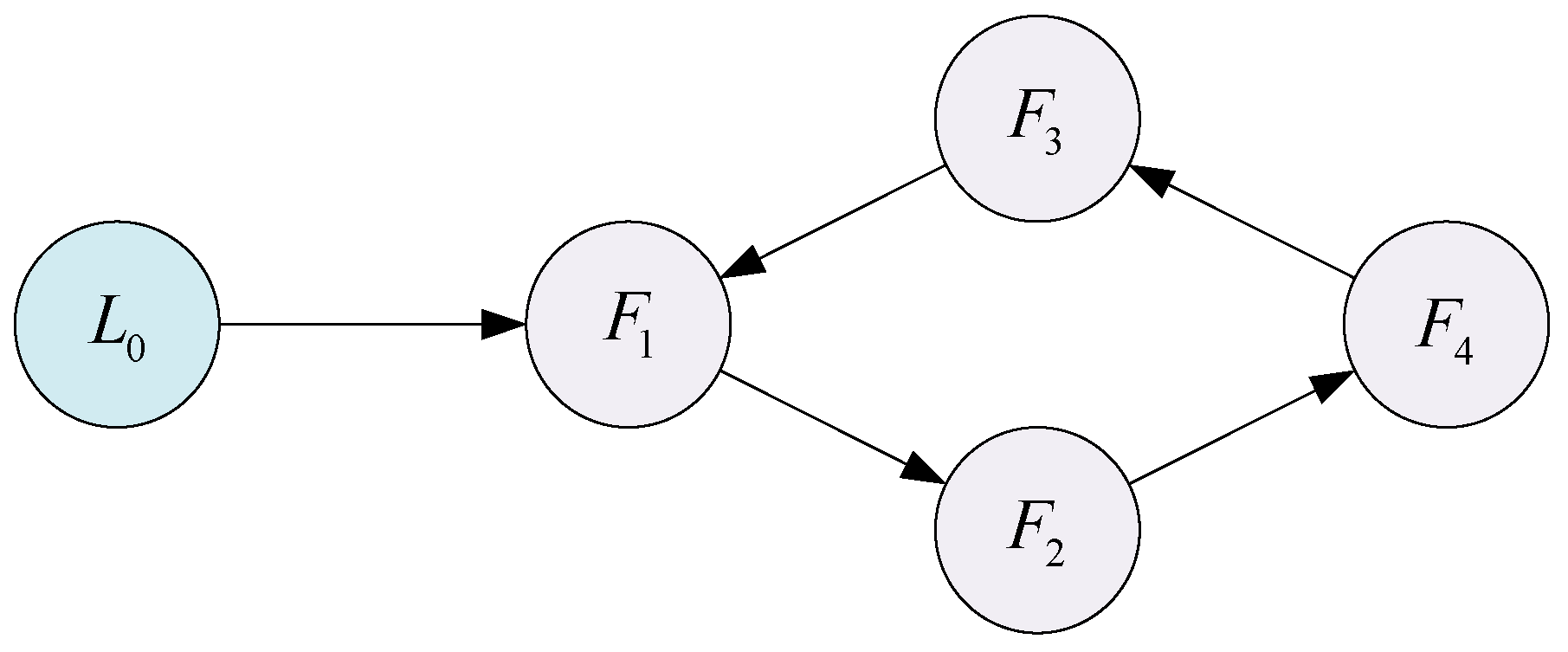
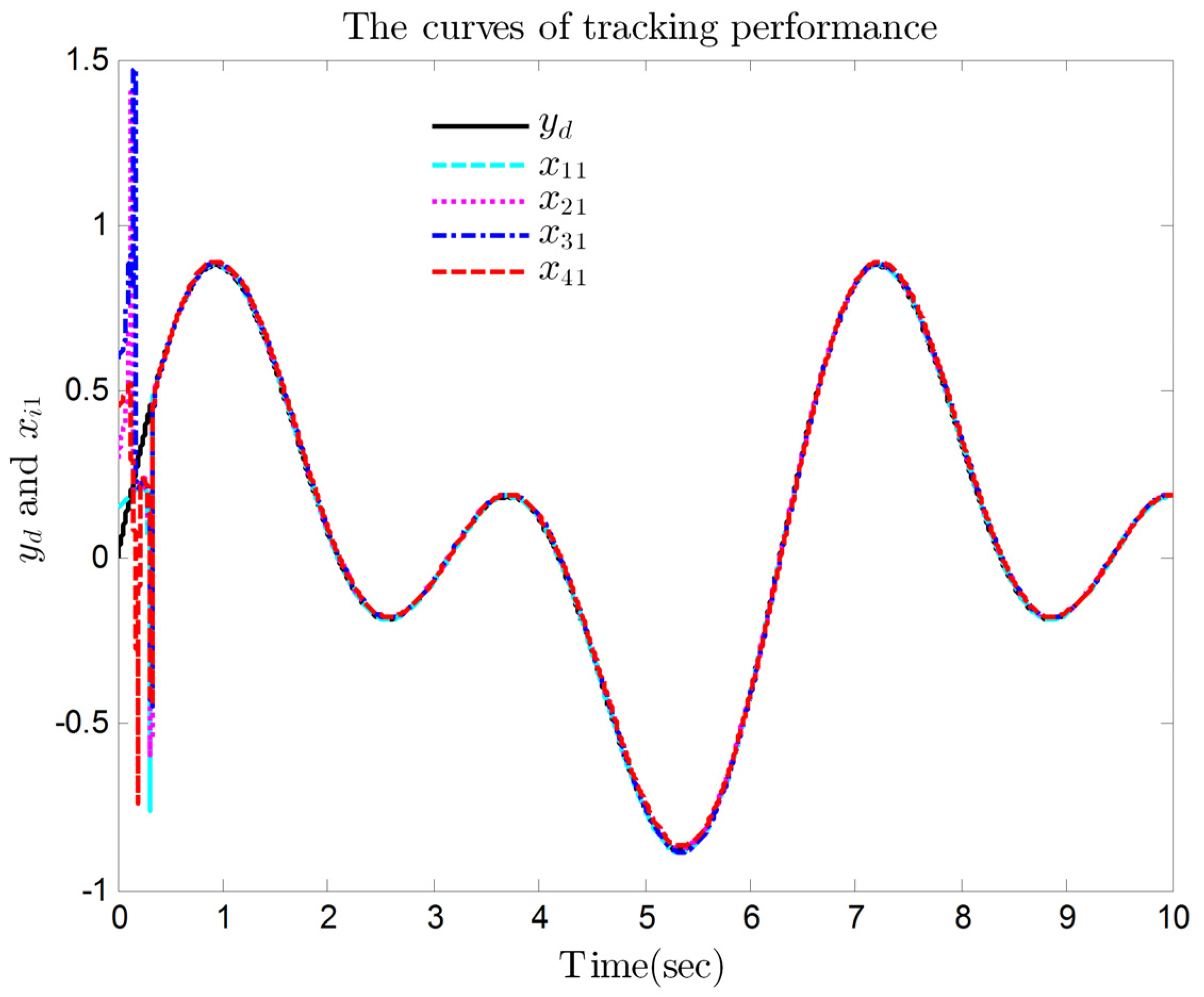
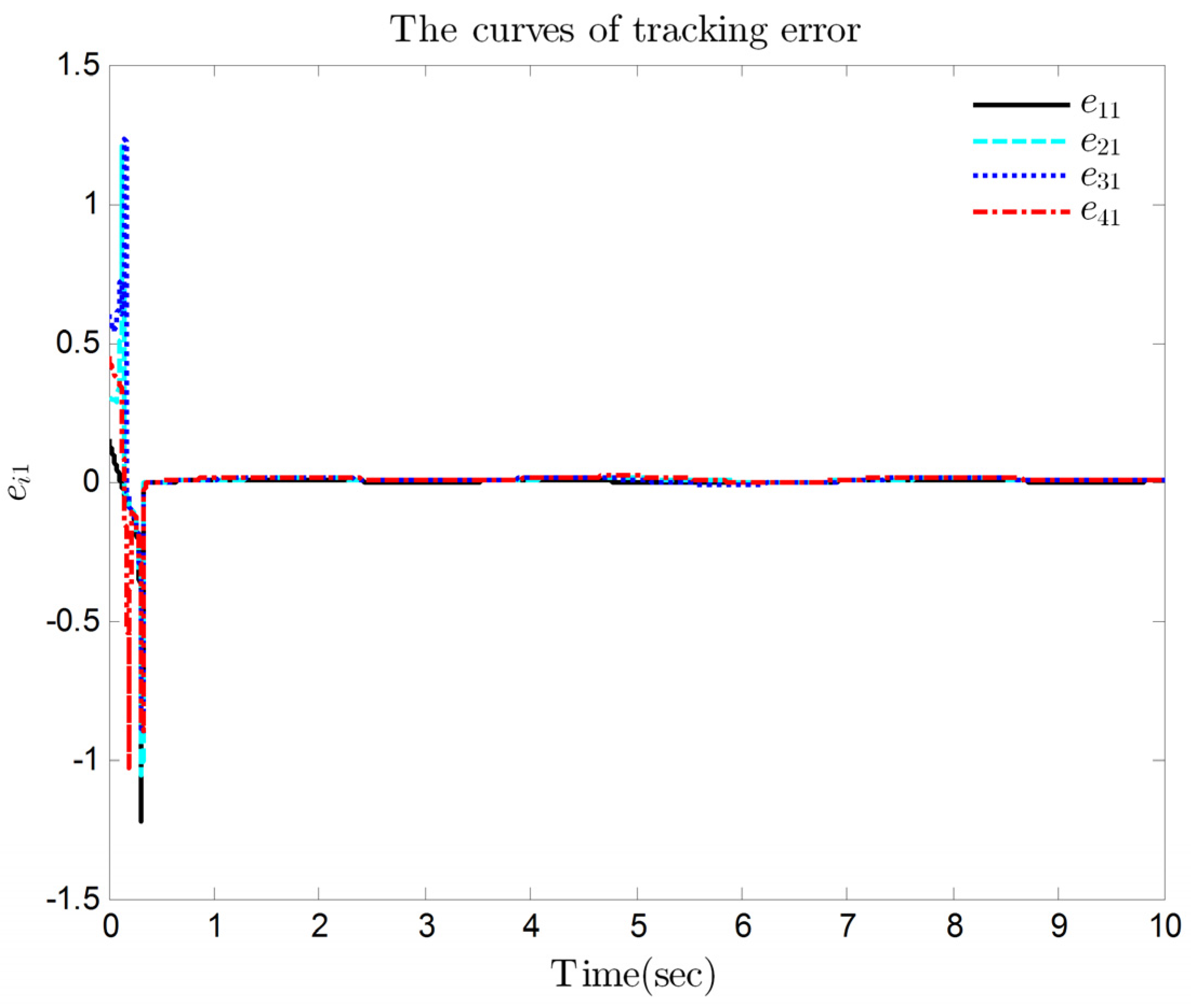
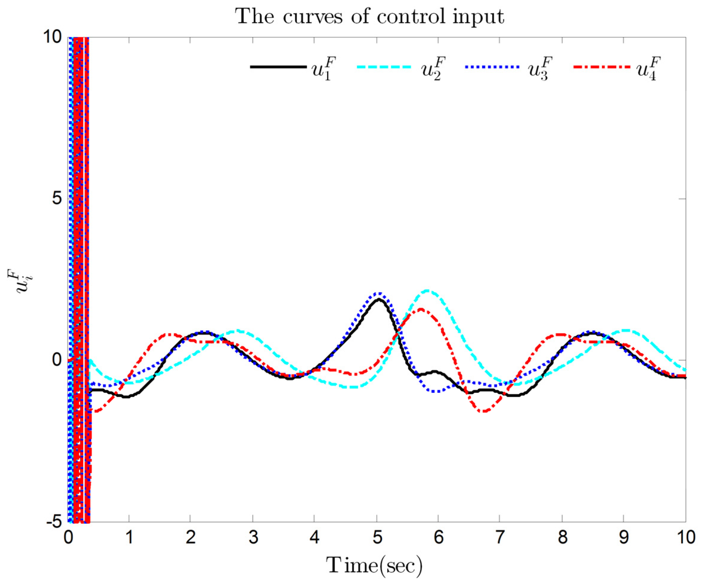
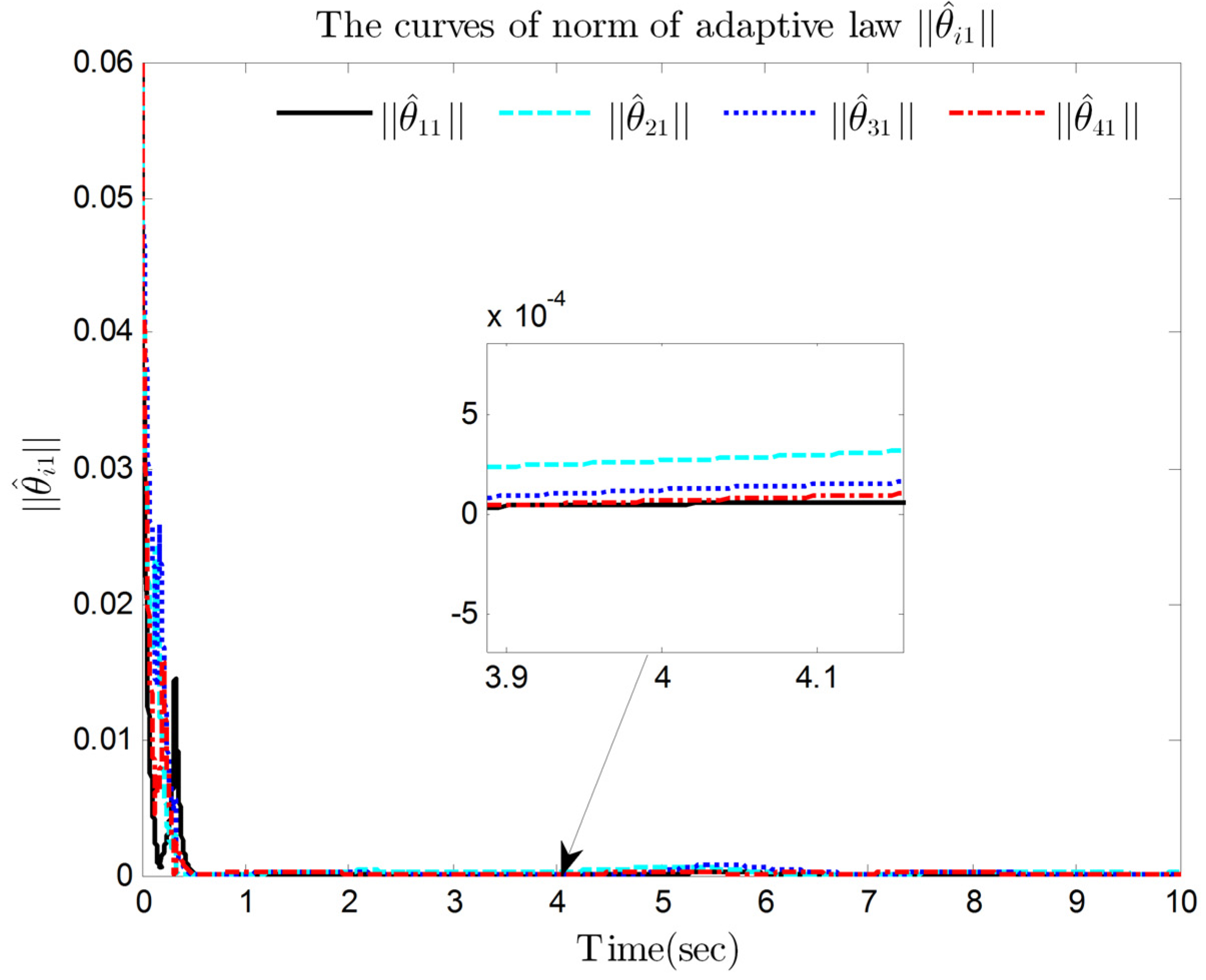
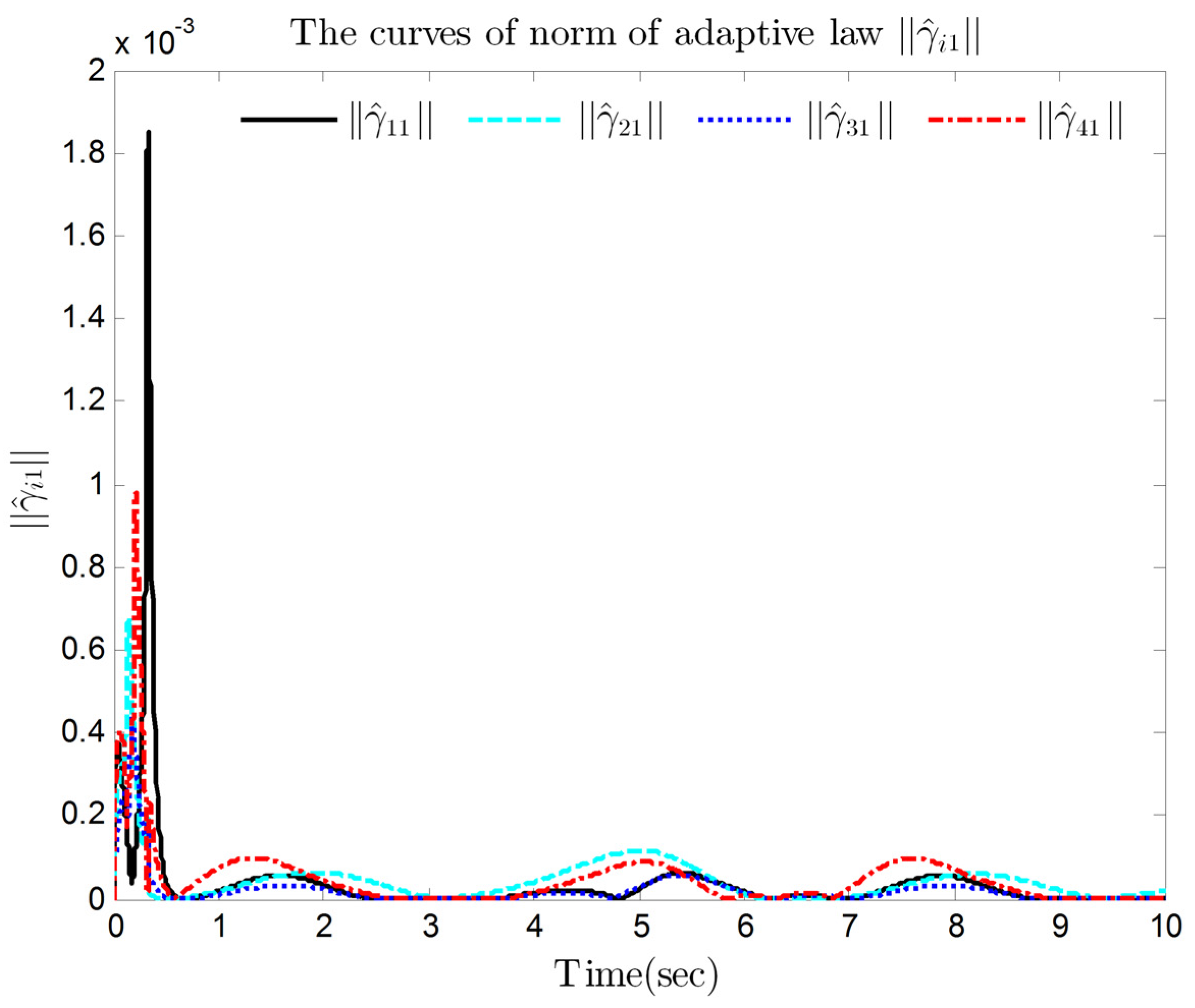
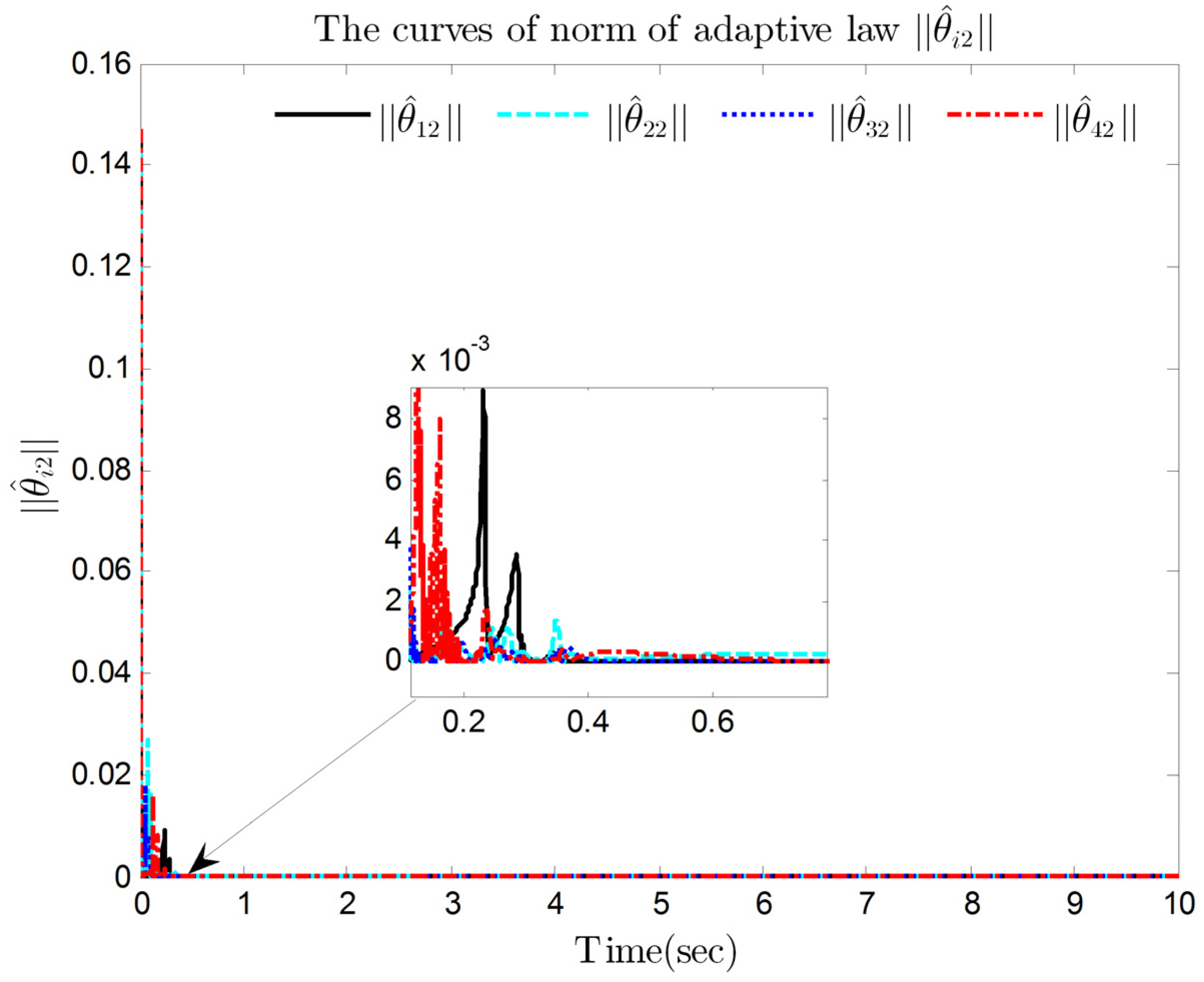
4. Simulation Results

To illustrate the validity of the proposed control law, the nonlinear multi-agent systems considered in this paper are described in (106). The system consists of one leader agent (Labeled L 0 ) and four follower agents (Labeled F 1 , F 2 , F 3 , and F 4 ), and the directed communication topology graph is shown in Figure 2.
x ˙ i , 1 = x i , 1 + f i , 1 ( x ¯ i , 1 ) + γ i , 1 T φ i , 1 ( x ¯ i , 1 ) x ˙ i , 2 = g i ( t ) u i F ( t ) + f i , 2 ( x ¯ i , 2 ) + γ i , 2 T φ i , 2 ( x ¯ i , 2 ) y i = x i , 1 ,   i = 1 , 2 , 3 , 4
where g 1 ( t ) = 0.6 + 0.4 sin ( t ) , g 2 ( t ) = 0.7 + 0.3 sin ( t ) , g 3 ( t ) = 0.8 + 0.2 sin ( t ) , g 4 ( t ) = 0.9 + 0.1 sin ( t ) , f 11 = 1.5 sin ( x 11 ) e ( x 11 3 ) , f 12 = x 11 cos ( x 12 ) , f 21 = 2 e ( x 21 ) , f 22 = 0.5 cos ( x 21 ) sin ( x 22 ) , f 31 = 1.5 x 31 e ( x 31 ) , f 32 = x 31 3 sin ( x 32 ) , f 41 = 2.5 x 41 sin ( x 41 ) , f 42 = 0.5 x 41 cos ( x 42 ) , φ 11 = [ x 11 , 0 ] T , φ 12 = [ x 12 , cos ( x 11 ) ] T , φ 21 = [ sin ( x 21 ) , x 21 ] T , φ 22 = [ 0 , sin ( x 21 ) cos ( x 22 ) ] T , φ 31 = [ cos 2 ( x 31 ) , 0 ] T , φ 32 = [ sin ( x 32 ) , x 31 sin ( x 31 ) ] T , φ 41 = [ x 41 , sin 2 ( x 41 ) ] T , φ 42 = [ 0 , x 41 cos ( x 42 ) ] T , γ i , 1 = γ i , 2 = [ 1.5 , 2 ] T .
The fuzzy logic system is applied to approximate the unknown nonlinear dynamics, and the membership functions are given as follows:
μ F i 1 ( x ) = exp ( ( x 3 ) 2 2 ) ,   μ F i 2 ( x ) = exp ( ( x 1.5 ) 2 2 ) ,   μ F i 3 ( x ) = exp ( x 2 2 ) μ F i 4 ( x ) = exp ( ( x + 1.5 ) 2 2 ) ,   μ F i 5 ( x ) = exp ( ( x + 3 ) 2 2 )
The initial states of the multi-agent systems (106) are set as x 11 = 0.15 , x 21 = 0.3 , x 31 = 0.6 , x 41 = 0.45 , and x 12 = x 22 = x 32 = x 42 = 0 . The initial values of the adaptive laws are given as ξ i , 1 ( 0 ) = ξ i , 2 ( 0 ) = 0 , κ i ( 0 ) = 0 , θ ^ i , 1 ( 0 ) = [ 0.01 ] 125 × 1 , θ ^ i , 2 ( 0 ) = [ 0.01 ] 25 × 1 , γ ^ i , 1 ( 0 ) = γ ^ i , j , 1 ( 0 ) = [ 0.01 ] 2 × 1 , γ ^ i , 2 ( 0 ) = [ 0.01 ] 2 × 1 , where i j = 1 , 2 , 3 , 4 . The desired reference trajectory is given as y d = 0.5 sin ( t ) + 0.5 sin ( 2 t ) , and the simulation time is set as t = 15   s .
The other design parameters were chosen as ϑ = 0.02 , ζ = 0.5 , ω i 2 = 2.5 , u i , min = 5 , u i , max = 10 , μ i = 0.9 , ε i 1 * = 0.2 , ε i 2 * = 0.1 , c i 1 = 8.5 , c i 2 = 10 , k i 1 = 12 , k i 2 = 15 , λ i 1 = 1.5 , λ i 2 = 2 , η i 1 = 2 , η i 2 = 3.5 , δ i j , 1 = 1.8 , Π i 1 = 9 , Π i 2 = 11 , Λ i 1 = 20 , Λ i 2 = 25 , Ψ i 1 = 25 , where i j = 1 , 2 , 3 , 4 .
Based on the designed control law and adaptive laws, the simulation results are shown in Figure 3, Figure 4, Figure 5, Figure 6, Figure 7, Figure 8, Figure 9 and Figure 10. The curves of the multi-agent systems outputs x i 1 and the reference trajectory y d are shown in Figure 3, and the tracking errors are given in Figure 4. As shown in Figure 3 and Figure 4, this paper showed that multi-agent systems can achieve a good tracking performance under the designed control law, and the tracking errors of four follower agents can converge to a small neighborhood of the origin in a finite time. Furthermore, observing Figure 3 and Figure 4, the multi-agent systems in this paper is subjected to unknown control directions and unknown input saturation, but the finite-time consensus tracking control problem can be solved by using designed control laws and adaptive laws. The curves of the saturated control input are displayed in Figure 5. It is not difficult to see that these control signals are within a limited range. In addition, this paper also presents the curves of the adaptive laws θ ^ i 1 , γ ^ i 1 , θ ^ i 2 , γ ^ i 2 and γ ^ i j , 1 , as shown in Figure 6, Figure 7, Figure 8, Figure 9 and Figure 10. Similarly, these signals are bounded. This also reflects the effectiveness of the control law designed in this paper from another point of view.

5. Conclusions

To solve the finite-time tracking control problem of a class of nonlinear multi-agent systems with unknown input saturation and unknown control directions, a command filter-based adaptive fuzzy finite-time control law has been proposed. The fuzzy logic systems have been applied to approximate each of the unknown nonlinear dynamics in the analysis process. To handle the command filter approximation errors, classes of compensating signals have been constructed in this paper, which effectively avoided the repeated differentiation of nonlinear functions in the recursive design process. Furthermore, considering the existence of unknown control directions and unknown input saturation, the Nussbaum gain function method has been utilized. Then, the effectiveness of the theoretical results is demonstrated through a numerical example. The results show that a good tracking performance can be obtained, and the tracking errors can converge to a sufficiently small neighborhood of the origin in finite time. To make the presented control law more effective, our future works will focus on the full state constraint problem of pure-feedback multi-agent systems with unknown control directions, and a class of observer-based control scheme should also be studied.

Author Contributions

Conceptualization, X.D.; Formal Analysis, X.D., Y.H. and L.W.; Funding Acquisition, X.D., Y.H. and L.W.; Investigation, X.D., Y.H. and L.W.; Methodology, Y.H. and L.W.; Project Administration, Y.H. and L.W.; Resources, X.D. and L.W.; Software, X.D. and Y.H.; Supervision, Y.H.; Validation, X.D.; Visualization, L.W.; Writing–original draft, X.D.; Writing–review and Editing, X.D., Y.H. and L.W. All authors have read and agreed to the published version of the manuscript.

Funding

This work was partially supported by the Natural Science Research of Colleges and Universities of Anhui Province under grant KJ2020A0344 and KJ2020ZD39, the Natural Science Foundation of Anhui Province under grant 2108085MF220, and the Program for the Top Talents of Anhui Polytechnic University.

Institutional Review Board Statement

Not applicable.

Informed Consent Statement

Not applicable.

Data Availability Statement

Not applicable.

Conflicts of Interest

The authors declare no conflict of interest.

Notations

In this paper, ( ) T represents transposing the vector or matrix ; R represents the set of real numbers; a i , min and a i , max represent the minimum value and the maximum value of variable a , respectively; diag { d 1 , , d n } represents a diagonal matrix with d 1 , , d n as diagonal elements; | B | represents the absolute value of constant B ; a represents the module of vector a ; C ^ represents the estimation of C * and C ˜ = C * C ^ stands for the estimation error; min { b 1 , , b n } and max { b 1 , , b n } represent the minimum value and maximum value of b 1 , , b n , respectively; and λ min ( A ) represents the smallest eigenvalue of A .

References

  1. Wang, B.; Chen, W.; Zhang, B.; Shi, P.; Zhang, H. A nonlinear observer-based approach to robust cooperative tracking for heterogeneous spacecraft attitude control and formation applications. IEEE Trans. Autom. Control 2022. [CrossRef]
  2. Li, Y.; Wu, Y.; He, S. Network-based leader-following formation control of second-order autonomous unmanned systems. J. Frankl. Inst. 2021, 358, 757–775. [Google Scholar] [CrossRef]
  3. Foderaro, G.; Zhu, P.; Wei, H.; Wettergren, T.A.; Ferrari, S. Distributed optimal control of sensor networks for dynamic target tracking. IEEE Trans. Control. Netw. Syst. 2018, 5, 142–153. [Google Scholar] [CrossRef]
  4. Zhang, P.; Xue, H.; Gao, S.; Zuo, X.; Zhang, J. Adaptive cooperative fault-tolerance tracking control for multi-agent system with hybrid actuator faults and multiple unknown control directions. Expert Syst. Appl. 2022, 197, 116711. [Google Scholar] [CrossRef]
  5. Chen, G.; Zhao, Y. Distributed adaptive output-feedback tracking control of non-affine multi-agent systems with prescribed performance. J. Frankl. Inst. 2018, 355, 6087–6110. [Google Scholar] [CrossRef]
  6. Zhang, S.; Chen, J.; Bai, C.; Li, J. Global iterative learning control based on fuzzy systems for nonlinear multi-agent systems with unknown dynamics. Inf. Sci. 2022, 587, 556–571. [Google Scholar] [CrossRef]
  7. Kaheni, M.; Usai, E.; Franceschelli, M. Resilient constrained optimization in multi-agent systems with improved guarantee on approximation bounds. IEEE Control. Lett. 2022, 6, 2659–2664. [Google Scholar] [CrossRef]
  8. Wen, G.; Zheng, W.X.; Wan, Y. Distributed robust optimization for networked agent systems with unknown nonlinearities. IEEE Trans. Autom. Control 2022. [Google Scholar] [CrossRef]
  9. Cao, X.; Zhang, C.; Zhao, D.; Sun, B.; Li, Y. Event-triggered consensus control of continuous-time stochastic multi-agent systems. Automatica 2022, 137, 110022. [Google Scholar] [CrossRef]
  10. Qian, Y.-Y.; Liu, L.; Feng, G. Distributed event-triggered adaptive control for consensus of linear multi-agent systems with external disturbances. IEEE Trans. Cybern. 2020, 50, 2197–2208. [Google Scholar] [CrossRef]
  11. Liu, G.; Zhou, Q.; Zhang, Y.; Liang, H. Fuzzy tracking control for nonlinear multi-agent systems with actuator faults and unknown control directions. Fuzzy Sets Syst. 2020, 385, 81–97. [Google Scholar] [CrossRef]
  12. Shamloo, N.F.; Kalat, A.A.; Chisci, L. Direct Adaptive Fuzzy Control of Nonlinear Descriptor Systems. Int. J. Fuzzy Syst. 2019, 21, 2588–2599. [Google Scholar] [CrossRef]
  13. Pan, T.-T.; Chang, X.-H.; Liu, Y. Robust Fuzzy Feedback Control for Nonlinear Systems With Input Quantization. IEEE Trans. Fuzzy Syst. 2022, 30, 4905–4914. [Google Scholar] [CrossRef]
  14. Zheng, S.; Shi, P.; Wang, S.; Shi, Y. Adaptive neural control for a class of nonlinear multiagent systems. IEEE Trans. Neural Netw. Learn. Syst. 2021, 32, 763–776. [Google Scholar] [CrossRef]
  15. Wang, F.; Gao, Y.; Zhou, C.; Zong, Q. Disturbance observer-based backstepping formation control of multiple quadrotors with asymmetric output error constraints. Appl. Math. Comput. 2022, 415, 126693. [Google Scholar] [CrossRef]
  16. Wu, W.; Tong, S. Fixed-time adaptive fuzzy containment dynamic surface control for nonlinear multi-agent systems. IEEE Trans. Fuzzy Syst. 2022, 30, 5237–5248. [Google Scholar] [CrossRef]
  17. Cui, Y.; Liu, X.; Deng, X.; Wen, G. Command-filter-based adaptive finite-time consensus control for nonlinear strict-feedback multi-agent systems with dynamic leader. Inf. Sci. 2021, 565, 17–31. [Google Scholar] [CrossRef]
  18. Deng, X.; Zhang, X. Adaptive fuzzy tracking control of uncertain nonlinear multi-agent systems with unknown control directions and a dead-zone fault. Mathematics 2022, 10, 2655. [Google Scholar] [CrossRef]
  19. Nussbaum, R.D. Some remarks on a conjecture in parameter adaptive control. Syst. Control. Lett. 1983, 3, 243–246. [Google Scholar] [CrossRef]
  20. Kamalamiri, A.; Shahrokhi, M.; Mohit, M. Adaptive finite-time neural control of non-strict feedback systems subject to output constraint, unknown control direction, and input nonlinearities. Inf. Sci. 2020, 520, 271–291. [Google Scholar] [CrossRef]
  21. Deng, X.; Zhang, C.; Ge, Y. Adaptive neural network dynamic surface control of uncertain strict-feedback nonlinear systems with unknown control direction and unknown actuator fault. J. Frankl. Inst. 2022, 359, 4054–4073. [Google Scholar] [CrossRef]
  22. Ma, J.; Xu, S.; Ma, Q.; Zhang, Z. Event-triggered adaptive neural network control for nonstrict-feedback nonlinear time-delay systems with unknown control directions. IEEE Trans. Neural Netw. Learn. Syst. 2020, 31, 4196–4205. [Google Scholar] [CrossRef]
  23. Cai, X.; Wang, C.; Wang, G.; Liang, D. Distributed consensus control for second-order nonlinear multi-agent systems with unknown control directions and position constraints. Neurocomputing 2018, 306, 61–67. [Google Scholar] [CrossRef]
  24. Fan, B.; Yang, Q.; Jagannathan, S.; Sun, Y. Output-constrained control of nonaffine multiagent systems with partially unknown control directions. IEEE Trans. Autom. Control 2019, 64, 3936–3942. [Google Scholar] [CrossRef]
  25. Zhang, Z.; Wang, C.; Cai, X. Consensus control of higher-order nonlinear multi-agent systems with unknown control directions. Neurocomputing 2019, 359, 122–129. [Google Scholar] [CrossRef]
  26. Ao, W.; Huang, J.; Xue, F. Adaptive leaderless consensus control of a class of strict-feedback nonlinear multi-agent systems with unknown control directions: A non-Nussbaum function based approach. J. Frankl. Inst. 2020, 357, 12180–12196. [Google Scholar] [CrossRef]
  27. Rezaee, H.; Abdollahi, F. Adaptive leaderless consensus control of strict-feedback nonlinear multiagent systems with unknown control directions. IEEE Trans. Syst. Man Cybern. Syst. 2021, 51, 6435–6444. [Google Scholar] [CrossRef]
  28. Li, Y.; Zhang, J.; Liu, W.; Tong, S. Observer-based adaptive optimized control for stochastic nonlinear systems with input and state constraints. IEEE Trans. Neural Netw. Learn. Syst. 2021, 33, 7791–7805. [Google Scholar] [CrossRef]
  29. Zhang, W.; Wei, W. Disturbance-observer-based finite-time adaptive fuzzy control for non-triangular switched nonlinear systems with input saturation. Inf. Sci. 2021, 561, 152–167. [Google Scholar] [CrossRef]
  30. He, C.; Wu, J.; Dai, J.; Zhang, Z. Fixed-time adaptive neural tracking control of output constrained nonlinear pure-feedback system with input saturation. Neurocomputing 2021, 451, 125–137. [Google Scholar] [CrossRef]
  31. Li, P.; Jabbari, F.; Sun, X.-M. Containment control of multi-agent systems with input saturation and unknown leader inputs. Automatica 2021, 130, 109677. [Google Scholar] [CrossRef]
  32. Zhu, Z.-H.; Guan, Z.-H.; Hu, B.; Zhang, D.-X.; Cheng, X.-M.; Li, T. Semi-global bipartite consensus tracking of singular multi-agent systems with input saturation. Neurocomputing 2021, 432, 183–193. [Google Scholar] [CrossRef]
  33. Cheng, W.; Xue, H.; Liang, H.; Wang, W. Prescribed performance adaptive fuzzy control of stochastic nonlinear multi-agent systems with input hysteresis and saturation. Int. J. Fuzzy Syst. 2022, 24, 91–104. [Google Scholar] [CrossRef]
  34. Zhao, L.; Yu, J.; Lin, C. Command filter based adaptive fuzzy bipartite output consensus tracking of nonlinear coopetition multi-agent systems with input saturation. ISA Trans. 2018, 80, 187–194. [Google Scholar] [CrossRef] [PubMed]
  35. Hao, R.; Wang, H.; Zheng, W. Dynamic event-triggered adaptive command filtered control for nonlinear multi-agent systems with input saturation and disturbances. ISA Trans. 2022, 130, 104–120. [Google Scholar] [CrossRef]
  36. Wang, H.; Chen, B.; Liu, X.; Liu, K.; Lin, C. Robust adaptive fuzzy tracking control for pure-feedback stochastic nonlinear systems with input constraints. IEEE Trans. Cybern. 2013, 43, 2093–2104. [Google Scholar] [CrossRef]
  37. Wang, M.; Liu, X.; Shi, P. Adaptive neural control of pure-feedback nonlinear time-delay systems via dynamic surface technique. IEEE Trans. Syst. Man Cybern. Part B (Cybernetics) 2011, 41, 1681–1692. [Google Scholar] [CrossRef]
  38. Hu, J.; Feng, G. Distributed tracking control of leader–follower multi-agent systems under noisy measurement. Automatica 2010, 46, 1382–1387. [Google Scholar] [CrossRef] [Green Version]
  39. Wang, F.; Chen, B.; Liu, X.; Lin, C. Finite-time adaptive fuzzy tracking control design for nonlinear systems. IEEE Trans. Fuzzy Syst. 2018, 26, 1207–1216. [Google Scholar] [CrossRef]
  40. Deng, X.; Wang, J. Fuzzy-based adaptive dynamic surface control for a type of uncertain nonlinear system with unknown actuator faults. Mathematics 2022, 10, 1624. [Google Scholar] [CrossRef]
  41. Yu, J.; Shi, P.; Dong, W.; Yu, H. Observer and command-filter-based adaptive fuzzy output feedback control of uncertain nonlinear systems. IEEE Trans. Ind. Electron. 2015, 62, 5962–5970. [Google Scholar] [CrossRef]
Figure 1. Control block diagram of multi-agent systems.
Mathematics 10 04656 g001
Figure 2. Communication topology graph of multi-agent systems.
Mathematics 10 04656 g002
Figure 3. Trracking results of four follower agents.
Mathematics 10 04656 g003
Figure 4. Tracking errors of four follower agents.
Mathematics 10 04656 g004
Figure 5. Control input u i F ( t ) .
Mathematics 10 04656 g005
Figure 6. Adaptive laws norm θ ^ i 1 .
Mathematics 10 04656 g006
Figure 7. Adaptive laws norm γ ^ i 1 .
Mathematics 10 04656 g007
Figure 8. Adaptive laws norm θ ^ i 2 .
Mathematics 10 04656 g008
Figure 9. Adaptive laws norm γ ^ i 2 .
Mathematics 10 04656 g009
Figure 10. Adaptive laws norm γ ^ i j , 1 .
Mathematics 10 04656 g010
Publisher’s Note: MDPI stays neutral with regard to jurisdictional claims in published maps and institutional affiliations.

