Article

Robust Synchronization of Fractional-Order Chaotic System Subject to Disturbances

1
Applied Technology College of Soochow University, Suzhou 215325, China
2
School of Mechanical and Electrical Engineering, Soochow University, Suzhou 215021, China
*
Author to whom correspondence should be addressed.
Mathematics 2022, 10(24), 4639; https://doi.org/10.3390/math10244639
Submission received: 16 November 2022 / Revised: 2 December 2022 / Accepted: 5 December 2022 / Published: 7 December 2022
(This article belongs to the Special Issue Dynamical System and Stochastic Analysis)

Abstract

:
This paper studies the synchronization problem for a class of chaotic systems subject to disturbances. The nonlinear functions contained in the master and slave systems are assumed to be incremental quadratic constraints. Under some assumptions, a feedback law is designed so that the error system behaves like the H performance. Meanwhile, the detailed algorithm for computing the incremental multiplier matrix is also given. Finally, one numerical example and one practical example are simulated to show the effectiveness of the designed method.

1. Introduction

The chaotic system is a kind of nonlinear system, and the characteristics of the chaotic system behave like the chaotic attractors. The definition of chaos was introduced by [1]. The investigation of the chaotic system has been paid much attention since it plays an important role in areas such as image encryption [2], fault detection [3], neural networks [4], communication security [5], and so on. In practice, the synchronization of master and slave chaotic systems is very essential to secure communication. Thus, synchronization has been studied extensively [6,7,8]. In [6], the authors used an active nonlinear controller to realize the synchronization of two hybrid chaotic systems, while [7] studied the design of adaptive controller for the purpose of the synchronization. Ref. [8] focused on the time-delay chaotic system, and a feedback law was designed to realize the robust synchronization. There were also other important works on synchronization for chaotic systems [9,10] herein.
On the other hand, the research on fractional-order systems is also a hot topic. The fractional-order system first appeared in a pure mathematical problem [11]. In the context of mathematics, Ref. [12] used the fractal-fractional mathematical model to describe the situation of corona virus, and [13] studied a class of nonlinear delayed corona virus pandemic model, while in [14], an optimal control problem of a nonholonomic macroeconomic system was investigated. Some researchers used the fractional-order system to describe more general practical systems. In fact, a fractional-order differential equation can be more accurate in describing complicated systems than integral-order differential equation. In the aspect of the fractional-order system, there were many interesting works, such as [15,16,17,18]. Since it is very powerful in describing more general systems, the study of fractional-order chaotic systems has always been a hot spot. Ref. [19] employed the active control method to investigate the synchronization problem for fractional-order chaotic systems, while, in [20], an adaptive impulsive controller was designed to achieve synchronization. The robust observer design problem for fractional-order chaotic systems was addressed in [21]. Moreover, the stability conditions of a class of impulsive incommensurate chaotic systems were analyzed in [22].
It should be noted that the nonlinear terms considered in the above-mentioned works [19,20,21,22] are all Lipschitz. Recently, a more general nonlinearity, called incremental quadratic constraints (IQC), has attracted much attention. It is pointed out in the work [23] that IQC is characterized by the incremental multiplier matrix (IMM) and can include Lipschitz constraints and one-sided Lipschitz constraints. The work [24] presented an observer design method for IQC systems, the results of [24] were extended to chaotic systems, and the secure communication problem was studied in [25]. Ref. [26] designed the controller for IQC systems with external disturbances. However, the robust synchronization of fractional-order chaotic systems under the framework of IQC has been reported rarely.
In the light of the above discussion, this paper considers the synchronization problem of fractional-order chaotic systems whose nonlinearity is described by IQC. The controller is designed by using the output, and the fractional-order stability theory is employed to derive sufficient conditions on robust synchronization. The remainder of the paper is as follows: Section 2 formulates the problem and presents some necessary basics. Section 3 designs the feedback law so that the robust synchronization is achieved. Section 4 suggests an algorithm to compute IMM. Section 5 simulates two examples to illustrate the validity of the designed method.

2. Preliminaries and Problem Statements

Consider the following fractional-order chaotic system:
D t α x ( t ) = A x ( t ) + G f ( H x ( t ) ) + D ω x ( t ) , z x ( t ) = C x ( t ) ,
where D t α is the α -order Caputo derivative with 0 < α < 1 . A R n × n , G R n × m , H R l × n , D R n × s , and C R q × n are constant matrices. x ( t ) R n is the system state, ω x ( t ) R s is the disturbance, and z x ( t ) R q is the output. f ( q ) : R l R m with q = H x ( t ) is the nonlinear function. For the purpose of simplification, the variable t is omitted when necessary. Then, the master system Equation (1) is written as:
D t a x = A x + G f ( H x ) + D ω x , z x = C x .
In the above system Equation (2), when the system matrices are given as:
A = 10 10 0 28 1 0 0 0 8 3 , G = 0 0 1 0 0 1 , H = 1 0 0 0 1 0 0 0 1 ,
f ( H x ) = x 1 x 3 x 1 x 2 , D = 1 0 0 , C = 1 0 0 .
The above fractional-order system behaves the chaos phenomenon. Figure 1 shows the phase plane of the system when α = 0.98 .
Then, the following slave system is presented:
D t a y = A y + G f ( H y ) + D ω y + B u , z y = C y ,
where ω y is the disturbance, and u is the controller, which is designed as u = K ( z y z x ) . Let e = y x , the error system is derived as follows:
D t a e = ( A + B K C ) e + G [ f ( H y ) f ( H x ) ] + D Δ ω .
where Δ ω = ω y ω x .
Denote that Γ ( α ) = 0 e t t α 1 d t . We firstly give the definitions of the fractional-order integral and derivative. More details can be found in [27].
Remark 1.
If the parameter errors exist in the system ( 1 ) , i.e., A and B will be substituted by A + Δ A ( t ) and B + Δ B ( t ) . Then, we can use the norm-bounded conditions of Δ A ( t ) and Δ B ( t ) to design the controller in ( 3 ) .
Definition 1 
([27]). A fractional integral of the function z with order α > 0 is defined as follows:
I t 0 α z ( t ) = 1 Γ ( α ) t 0 t ( t s ) α 1 z ( s ) d s .
Definition 2
([27]). A Caputo fractional derivative of the function z with order 0 < α < 1 is defined as follows:
D t α z ( t ) = 1 Γ ( α ) 0 t ( t s ) α d d s z ( s ) d s .
Definition 3
([24]). For a nonlinear function φ ( θ ) , if there exists a symmetric matrix W such that
θ 1 θ 2 φ ( θ 1 ) φ ( θ 2 ) T W θ 1 θ 2 φ ( θ 1 ) φ ( θ 2 ) 0 ,
then φ ( θ ) is IQC, and W is called the IMM for φ ( θ ) .
From [24], it is known that Lispchitz constraints or one-sided Lipschitz constraints are a special case of IQC.
Definition 4
([28]). The error system ( 4 ) behaves the H performance, if
( 1 ) Δ ω = 0 , lim t e ( t ) = 0 ;
( 2 ) Δ ω 0 ; under the zero-initial condition, the following inequality holds:
0 e T ( s ) e ( s ) d s < ς 0 Δ ω T ( s ) Δ ω ( s ) d s ,
where ς > 0 is the disturbance attenuation level.
Assumption A1.
The nonlinear function f ( q ) in systems (2) and (3) satisfies IQC with IMM M, i.e.,
q 2 q 1 f ( q 2 ) f ( q 1 ) T M q 2 q 1 Φ 1 ( q 2 ) Φ 1 ( q 1 ) 0 ,
and M has the blocked form as follows:
M = M 11 M 12 M 21 M 22 ,
where M 11 R n × n and M 22 R s × s .
Lemma 1
([29]). Let V ( t ) = x T ( t ) P x ( t ) be a continuously differentiable function, then D t α V ( t ) satisfies:
D t α V ( t ) ( D t α e ( t ) ) T P e ( t ) + e T P ( D t α e ( t ) ) .

3. Main Results

We first state the following theorem, where sufficient conditions are given so that the controller design is effective.
Theorem 1.
Let Assumption A1 hold. If matrices P = P T > 0 and K exist such that
( A + B K C ) T P + P ( A + B K C ) + I + H T M 11 H P G + H T M 12 P D G T P + M 21 H M 22 0 D T P 0 ς I < 0 ,
where ς > 0 is the disturbance attenuation level, then the error system Equation (4) behaves like the H performance, i.e., the robust synchronization of systems Equations (2) and (3) is achieved.
Proof. 
Consider the following Lyapunov function candidate:
V = e T P e .
From Lemma 1, the fractional derivative of V is
D t α V ( D t α e T ) P e + e T P D t α e .
Thus, along the error dynamics Equation (4), we have
D t α V e T [ ( A + B K C ) T P + P ( A + B K C ) ] e + e T P D Δ ω + Δ ω T D T P e e T P G [ f ( H y ) f ( H x ) ] + [ f ( H y ) f ( H x ) ] T G T P e .
The proof is divided into two steps according to Definition 4.
( i ) Δ ω ( t ) = 0 . It follows from Equation (12) that
D t α V e T [ ( A + B K C ) T P + P ( A + B K C ) ] e e T P G [ f ( H y ) f ( H x ) ] + [ f ( H y ) f ( H x ) ] T G T P e .
Define that δ = f ( H y ) f ( H x ) , by using Assumption A1, we have
e δ T H T 0 0 I M H 0 0 I e δ 0 ,
i.e.,
e δ T H T M 11 H H T M 12 M 21 H M 22 e δ 0 .
Denote that ξ = [ e T δ T ] T . Substituting Equation (14) into Equation (13) yields
D t α V ξ T Λ ξ ,
where
Λ = ( A + B K C ) T P + P ( A + B K C ) + H T M 11 H P G + H T M 12 G T P + M 21 H M 22 .
In view of Equation (9), by using the matrix theory, we have
( A + B K C ) T P + P ( A + B K C ) + I + H T M 11 H P G + H T M 12 G T P + M 21 H M 22 < 0 .
Thus, Γ < 0 . From Equation (15), we can deduce that D t α V < 0 , which means that lim t e ( t ) = 0 .
(ii) Δ ω ( t ) 0 . Let
J = 0 e T ( t ) e ( t ) d t 0 ς ω T ( t ) ω ( t ) d t = 0 [ e T ( t ) e ( t ) ς ω T ( t ) ω ( t ) ] d t .
Recall that
I 0 1 D t α V ( e ) = I 0 1 α I 0 α D t α V ( e ) ,
then
I 0 1 D t α V ( e ) = I 0 1 α ( V ( e ( t ) ) V ( e ( 0 ) ) ) .
By using the zero-initial condition e ( 0 ) = 0 , one gets
I 0 1 D t α V ( e ) = I 0 1 α ( V ( e ( t ) ) ) .
Since V ( e ( t ) ) 0 , we have 0 1 α ( V ( e ( t ) ) ) 0 , i.e., 0 1 D t α V ( e ) 0 , which implies that
0 D α t V ( t ) d t 0 .
Thus, it follows from Equations (16) and (20) that
J 0 [ e T ( t ) e ( t ) ς ω T ( t ) ω ( t ) + D α t V ( t ) ] d t .
Denote that S = e T e ς ω T ω + D α t V , together with Equation (12), we have
S = e T e ς ω T ω + e T [ ( A + B K C ) T P + P ( A + B K C ) ] e + δ T G T P e + e T P G δ + Δ ω T D T P e + e T P D Δ ω .
Define that ζ = [ e T δ T Δ ω T ] T . Substituting Equation (14) into Equation (22) yields
S ζ T Θ ζ ,
where
Θ = ( A + B K C ) T P + P ( A + B K C ) + I + H T M 11 H P G + H T M 12 P D G T P + M 21 H M 22 0 D T P 0 ς I .
It follows from Equations (9), (19) and (23) that
J 0 S ( t ) d t < 0 ,
which implies
0 e T ( t ) e ( t ) d t 0 ς ω T ( t ) ω ( t ) d t < 0 ,
i.e.,
0 e T ( t ) e ( t ) d t < ς 0 ω T ( t ) ω ( t ) d t .
Combining (i) with (ii), the proof is completed. □
Remark 2.
The condition Equation (9) cannot be solved by the Matlab LMI toolbox since it is not a standard LMI. Here, one solution is suggested to deal with the matrix inequality Equation (9). Let P B K = Z ; then Equation (9) is equivalent to
A T P + P A + Z C + C T Z T + I + H T M 11 H P G + H T M 12 P D G T P + M 21 H M 22 0 D T P 0 ς I < 0 .
Thus, we can use the Matlab LMI toolbox to solve the matrix P from Equation (27). Then, if r a n k ( P B ) = r a n k ( P B Z ) , then K = ( P B ) Z , where ( P B ) is the Moore inverse matrix of P B .

4. The Determination of IMM M

In Equation (27), the matrix M is essential to the solutions P and K. Thus, we will give a detailed algorithm to compute M in this section. Generally, the nonlinear function f ( q ) in system Equations (2) and (3) is supposed to be continuously differentiable, and it is characterized by a known set Ω of matrices. For any q 1 , q 2 R l , there is a matrix Υ in Ω such that f ( q 1 ) f ( q 2 ) = Υ ( q 1 q 2 ) . Ω is a known polytope of matrices with vertices Υ 1 , Υ 2 , …, Υ n denoted by Ω = c o { Υ 1 , Υ 2 , , Υ n } . By using IQC, one gets
I Υ i T M I Υ i 0 , i I [ 1 , N ] .
In view of the decomposition form of M, Equation (28) becomes
M 11 + M 12 Υ i + Υ i T M 12 T + Υ i T M 22 Υ i 0 , i I [ 1 , N ] .
By using the Shur complements, we have
M 11 + M 12 Υ i + Υ i T M 12 T Υ i T M 22 M 22 Υ i M 22 0 , i I [ 1 , N ] .
By solving Equation (29), the solution M may be found. However, it is not easy to determine Y i . In the sequel, we provide a method with to compute these vertex matrices Υ i of f ( q ) in systems Equations (2) and (3). Since f ( q ) is continuously differentiable, then
f ( q ) q = q 3 0 q 1 q 2 q 1 0 = x 3 0 x 1 x 2 x 1 0 = x 1 0 0 1 0 1 0 + x 2 0 0 0 1 0 0 + x 3 1 0 0 0 0 0 .
Thus, the vertices of the polytope Ω can be described by
Υ 1 = τ 0 0 1 0 1 0 , Υ 2 = τ 0 0 0 1 0 0 , Υ 3 = τ 1 0 0 0 0 0 , Υ 4 = τ 0 0 1 0 1 0 , Υ 5 = τ 0 0 0 1 0 0 , Υ 6 = τ 1 0 0 0 0 0 ,
By using the bounded condition in [30], we solve Equation (29) and have
M 11 = 10.1989 0 0 0 7.9306 0 0 0 7.4134 , M 12 = 0.952 0 0 1.4586 0 0 ,
M 22 = 4.0588 0 0 4.0836 .
Remark 3.
By the definition of IQC, we know that the matrix M may have infinite solutions. To some extent, the computation of M is not an easy task. The detailed procedure depends on the parameter τ. Owing to the technique proposed in [30], the detailed computation process of τ is omitted here.

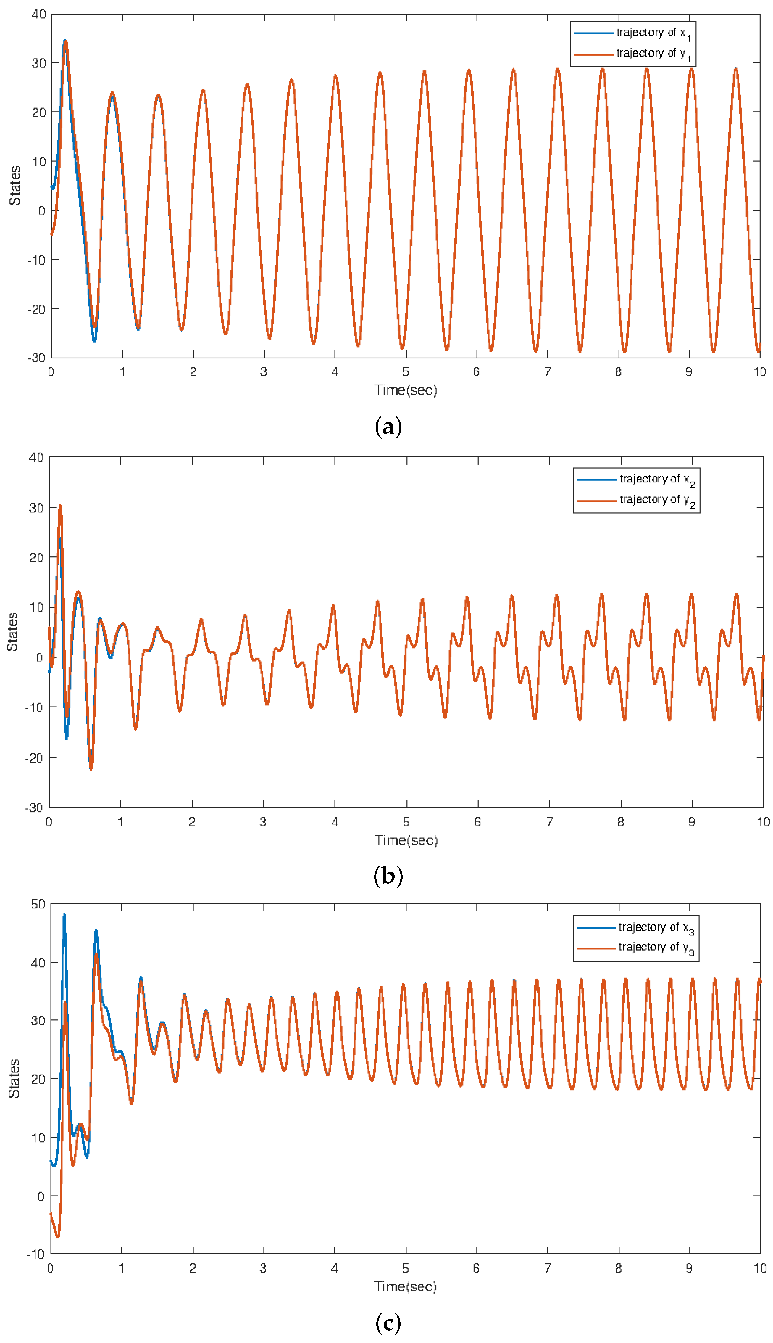
5. Numerical Simulation

Example 1.
Consider the system Equation (2) with the matrix parameters:
A = 10 10 0 28 1 0 0 0 8 3 , G = 0 0 1 0 0 1 , H = 1 0 0 0 1 0 0 0 1 ,
f ( H x ) = x 1 x 3 x 1 x 2 , D = 1 0 0 , C = 1 0 0 .
By using the results of the fractional order system, if α 0.98 , the system Equation (2) behaves like chaotic attractors. Therefore, α is setting as 0.98 in the simulation. We solve IMM for f ( H x ) , and M is given as shown in Equation (30). The disturbances ω x and ω y are as follows:
ω x = ω y = 300 sin ( 10 t ) , 0 t 3 s , 0 , t > 3 s .
The initial values of x and y are chosen as
x T ( 0 ) = 5 3 6 , y T ( 0 ) = 5 6 3 .
First, we deal with nonlinearity through the I M M algorithm in Section 4, and the matrix M is as follows:
M = 10.1989 0 0 0.9520 0 0 7.9306 0 0 1.4586 0 0 7.4134 0 0 0.9520 0 0 4.0588 0 0 1.4586 0 0 4.0836 .
We let
0 e T ( t ) e ( t ) d t < 5 0 ω T ( t ) ω ( t ) d t ,
when Δ ω ( t ) 0 . Substituting M into Equation (27) yields
P = 6.0584 0.5478 0.1606 0.5478 2.0698 0.4468 0.1606 0.4468 2.6717 ,
which can be seen that P is positive definite. Furthermore, we have
Z = 67.2326 124.5635 10.4750 .
It is obvious that r a n k ( P B ) = r a n k ( P B Z ) , i.e., K = ( P B ) Z , where ( P B ) is the Moore inverse matrix of P B . Hence, the controller gain can be obtained
K = 5.5223 59.9667 5.7749 .
During the simulation, we denote that
x = x 1 x 2 x 3 , y = y 1 y 2 y 3 , e = e 1 e 2 e 3 .
In Figure 2, the trajectories of each state of system Equation (2) and system Equation (3) are shown. In Figure 3, the trajectories of error dynamics e ( t ) are shown. It can be seen that the trajectories of errors exhibit bounded convergence under the influence of disturbances ω x and ω y in the first 3 s. However, after 3 s, when the disturbances disappears, the error will gradually converge to zero. It is consistent with the theoretical results. Thus, the proposed method is valid in this paper.
Example 2.
Fractional-order Lorentz systems can be used to describe a class of circuit systems. In Figure 4, the three state variables x, y, and z are implemented by three channels, respectively, and some of these calculus operations are replaced by operational amplifiers and analog multipliers. The resistors in Figure 4 are R i = 10 k Ω ; i = 1 , 2 , 8 , 9 , 12 , 13 , 15 , 16 , 18 , 19 , 21 , 22 ; R 4 = 1 k Ω ; R 5 = 1.55 M Ω ; R 6 = 62 M Ω ; R 7 = 2.5 k Ω ; R 10 = 3.57 k Ω ; R j = 100 k Ω ; j = 11 , 14 , 20 ; and R 17 = 37.5 k Ω ; R 3 is adjustable, and the capacitors are C 1 = 0.73 μ F , C 2 = 0.52 μ F , C 3 = 1.1 μ F , C 4 = C 5 = 1 n F . By adjusting R 3 , different chaotic phenomena can be obtained.
From [31], by analyzing the circuit system in Figure 4, we obtain the following state-space dynamics:
D t α x ( t ) = A x ( t ) + G f ( H x ( t ) ) + D ω x ( t ) , z x ( t ) = C x ( t ) ,
where
A = 10 10 0 28 1 0 0 0 8 3 , G = 0 0 1 0 0 1 , H = 1 0 0 0 1 0 0 0 1 ,
f ( H x ) = x 1 x 3 x 1 x 2 , D = 1 0 0 0 1 0 0 0 0 , C = 1 0 0 .
The disturbance is chosen as:
w x = w y = 10 s i n ( 10 t ) 20 s i n ( 10 t ) 0 , 0 t 10 s , 0 , t > 10 s .
Then, the control gain K is obtained by solving Equation (27)
K = 3.6982 53.0802 4.1746 ,
and
P = 1.7077 0.5876 0.1182 0.5876 1.0806 0.3321 0.1182 0.3321 2.4589 , Z = 25.3700 53.7972 7.8021 .
The state trajectories of three variables in the circuit system are depicted in Figure 5, and the trajectories of the tracking errors between the master–slave circuit systems are shown in Figure 6. The simulation results are consistent with the theoretical results.
Remark 4.
In [18], the sliding mode control problem for fractional-order systems was considered. Unlike [18], the synchronization problem for fractional-order chaotic systems is concerned in this paper. Moreover, compared with [19,20,21,22], the nonlinearity in this paper satisfies IQC, and it is a more gerenal description.

6. Conclusions

The robust synchronization problem of nonlinear fractional-order chaotic systems was investigated in this paper. Under the framework of IQC, the nonlinear function was described by using the IMM and state variables. The detailed computation method for IMM was also presented when the nonlinearity in chaotic system was concerned. Under the sufficient conditions, the controller was designed so that the error system behaved like the H performance. At last, two examples were given to verify the validity of the proposed method. In future work, we will focus on the adaptive control or another advanced control for fractional-order chaotic systems.

Author Contributions

Methodology, X.Z.; Software, S.W.; Writing—original draft, D.L.; Supervision, F.Y. All authors have read and agreed to the published version of the manuscript.

Funding

This research received no external funding.

Institutional Review Board Statement

Not applicable.

Informed Consent Statement

Not applicable.

Data Availability Statement

Not applicable.

Conflicts of Interest

The authors declare no conflict of interest.

References

  1. Ott, E.; Grebogi, C.; Yorke, J.A. Controlling chaos. Phys. Rev. Lett. 1990, 64, 1196. [Google Scholar] [CrossRef] [PubMed]
  2. Wang, X.; Teng, L.; Qin, X. A novel colour image encryption algorithm based on chaos. Signal Process. 2012, 92, 1101–1108. [Google Scholar] [CrossRef]
  3. Du, Y.; Duever, T.A.; Budman, H. Fault detection and diagnosis with parametric uncertainty using generalized polynomial chaos. Comput. Chem. Eng. 2015, 76, 63–75. [Google Scholar] [CrossRef]
  4. Potapov, A.; Ali, M. Robust chaos in neural networks. Phys. Lett. A 2000, 277, 310–322. [Google Scholar] [CrossRef]
  5. Cheng, C.J. Robust synchronization of uncertain unified chaotic systems subject to noise and its application to secure communication. Appl. Math. Comput. 2012, 219, 2698–2712. [Google Scholar] [CrossRef]
  6. Vaidyanathan, S. Hybrid chaos synchronization of Liu and Lü systems by active nonlinear control. In Proceedings of the International Conference on Computational Science, Engineering and Information Technology, Tirunelveli, India, 23–25 September 2011; pp. 1–10. [Google Scholar]
  7. Ahn, C.K.; Jung, S.T.; Kang, S.K.; Joo, S.C. Adaptive H synchronization for uncertain chaotic systems with external disturbance. Commun. Nonlinear Sci. Numer. Simul. 2010, 15, 2168–2177. [Google Scholar] [CrossRef]
  8. Zhao, Z.; Lv, F.; Zhang, J.; Du, Y. H synchronization for uncertain time-delay chaotic systems with one-sided lipschitz nonlinearity. IEEE Access 2018, 6, 19798–19806. [Google Scholar] [CrossRef]
  9. Pecora, L.M.; Carroll, T.L. Synchronization in chaotic systems. Phys. Rev. Lett. 1990, 64, 821. [Google Scholar] [CrossRef]
  10. Olusola, O.I.; Vincent, E.; Njah, A.N.; Ali, E. Control and synchronization of chaos in biological systems via backsteping design. Int. J. Nonlinear Sci. 2011, 11, 121–128. [Google Scholar]
  11. Oldham, K.; Spanier, J. The Fractional Calculus Theory and Applications of Differentiation and Integration to Arbitrary Order; Elsevier: Amsterdam, The Netherlands, 1974. [Google Scholar]
  12. Shah, K.; Arfan, M.; Mahariq, I.; Ahmadian, A.; Salahshour, S.; Ferrara, M. Fractal-fractional mathematical model addressing the situation of corona virus in Pakistan. Results Phys. 2020, 19, 103560. [Google Scholar] [CrossRef]
  13. Raza, A.; Ahmadian, A.; Rafiq, M.; Salahshour, S.; Ferrara, M. An analysis of a nonlinear susceptible-exposed-infected-quarantine-recovered pandemic model of a novel coronavirus with delay effect. Results Phys. 2021, 21, 103771. [Google Scholar] [CrossRef] [PubMed]
  14. Udrişte, C.; Ferrara, M.; Zugrăvescu, D.; Munteanu, F. Controllability of a nonholonomic macroeconomic system. J. Optim. Theory Appl. 2012, 154, 1036–1054. [Google Scholar] [CrossRef]
  15. Tavazoei, M.S.; Haeri, M. A note on the stability of fractional order systems. Math. Comput. Simul. 2009, 79, 1566–1576. [Google Scholar] [CrossRef]
  16. Li, M.; Li, D.; Wang, J.; Zhao, C. Active disturbance rejection control for fractional-order system. ISA Trans. 2013, 52, 365–374. [Google Scholar] [CrossRef]
  17. Zheng, S. Robust stability of fractional order system with general interval uncertainties. Syst. Control Lett. 2017, 99, 1–8. [Google Scholar] [CrossRef]
  18. Kamal, S.; Sharma, R.K.; Dinh, T.N.; Ms, H.; Bandyopadhyay, B. Sliding mode control of uncertain fractional-order systems: A reaching phase free approach. Asian J. Control 2021, 23, 199–208. [Google Scholar] [CrossRef]
  19. Agrawal, S.; Srivastava, M.; Das, S. Synchronization of fractional order chaotic systems using active control method. Chaos Solitons Fractals 2012, 45, 737–752. [Google Scholar] [CrossRef]
  20. Andrew, L.Y.T.; Xian-Feng, L.; Yan-Dong, C.; Hui, Z. A novel adaptive-impulsive synchronization of fractional-order chaotic systems. Chin. Phys. B 2015, 24, 100502. [Google Scholar] [CrossRef]
  21. N Doye, I.; Salama, K.N.; Laleg-Kirati, T.M. Robust fractional-order proportional-integral observer for synchronization of chaotic fractional-order systems. IEEE/CAA J. Autom. Sin. 2019, 6, 268–277. [Google Scholar] [CrossRef]
  22. Luo, R.; Su, H. The stability of impulsive incommensurate fractional order chaotic systems with Caputo derivative. Chin. J. Phys. 2018, 56, 1599–1608. [Google Scholar] [CrossRef]
  23. D’Alto, L.; Corless, M. Incremental quadratic stability. Numer. Algebra Control Optim. 2013, 3, 175–201. [Google Scholar] [CrossRef]
  24. Açıkmeşe, B.; Corless, M. Observers for systems with nonlinearities satisfying incremental quadratic constraints. Automatica 2011, 47, 1339–1348. [Google Scholar] [CrossRef]
  25. Zhao, Y.; Zhang, W.; Su, H.; Yang, J. Observer-based synchronization of chaotic systems satisfying incremental quadratic constraints and its application in secure communication. IEEE Trans. Syst. Man Cybern. Syst. 2018, 1–12. [Google Scholar] [CrossRef]
  26. Xu, X.; Açıkmeşe, B.; Corless, M.J. Observer-Based Controllers for Incrementally Quadratic Nonlinear Systems With Disturbances. IEEE Trans. Autom. Control. 2021, 66, 1129–1143. [Google Scholar] [CrossRef]
  27. Podlubny, I. Fractional Derivatives and Integrals. In Fractional Differential Equations: An Introduction to Fractional Derivatives; Elsevier: Amsterdam, The Netherlands, 1998; pp. 41–80. [Google Scholar]
  28. Xiang, W.; Xiao, J.; Iqbal, M.N. Robust observer design for nonlinear uncertain switched systems under asynchronous switching. Nonlinear Anal. Hybrid Syst. 2012, 6, 754–773. [Google Scholar] [CrossRef]
  29. Zhang, H.; Huang, J.; He, S. Fractional-Order Interval Observer for Multiagent Nonlinear Systems. Fractal Fract. 2022, 6, 355. [Google Scholar] [CrossRef]
  30. Li, D.; Lu, J.; Wu, X.; Chen, G. Estimating the bounds for the Lorenz family of chaotic systems. Chaos Solitons Fractals 2005, 23, 529–534. [Google Scholar] [CrossRef]
  31. Jia, H.; Tao, Q.; Chen, Z. Analysis and circuit design of a fractional-order Lorenz system with different fractional orders. Syst. Sci. Control Eng. Open Access J. 2014, 2, 745–750. [Google Scholar] [CrossRef]
Figure 1. The chaotic behavior of fractional-order chaotic system.
Mathematics 10 04639 g001
Figure 2. The trajectories of x ( t ) and y ( t ) , (a) the trajectories of x 1 and y 1 , (b) the trajectories of x 2 and y 2 , and (c) the trajectories of x 3 and y 3 .
Mathematics 10 04639 g002
Figure 3. The trajectory of tracking error e ( t ) , (a) The trajectory of tracking error e 1 , (b) the trajectory of tracking error e 2 , and (c) the trajectory of tracking error e 3 .
Mathematics 10 04639 g003
Figure 4. Analog circuit of the fractional-order Lorenz system.
Mathematics 10 04639 g004
Figure 5. The trajectories of x ( t ) and y ( t ) , (a) the trajectories of x 1 and y 1 , (b), the trajectories of x 2 and y 2 , and (c) the trajectories of x 3 and y 3 .
Mathematics 10 04639 g005
Figure 6. The trajectory of tracking error e ( t ) , (a) the trajectory of tracking error e 1 , (b) the trajectory of tracking error e 2 , and (c) the trajectory of tracking error e 3 .
Mathematics 10 04639 g006
Publisher’s Note: MDPI stays neutral with regard to jurisdictional claims in published maps and institutional affiliations.

