
A Two-Dimensional port-Hamiltonian Model for Coupled Heat Transfer

Abstract
:1. Introduction
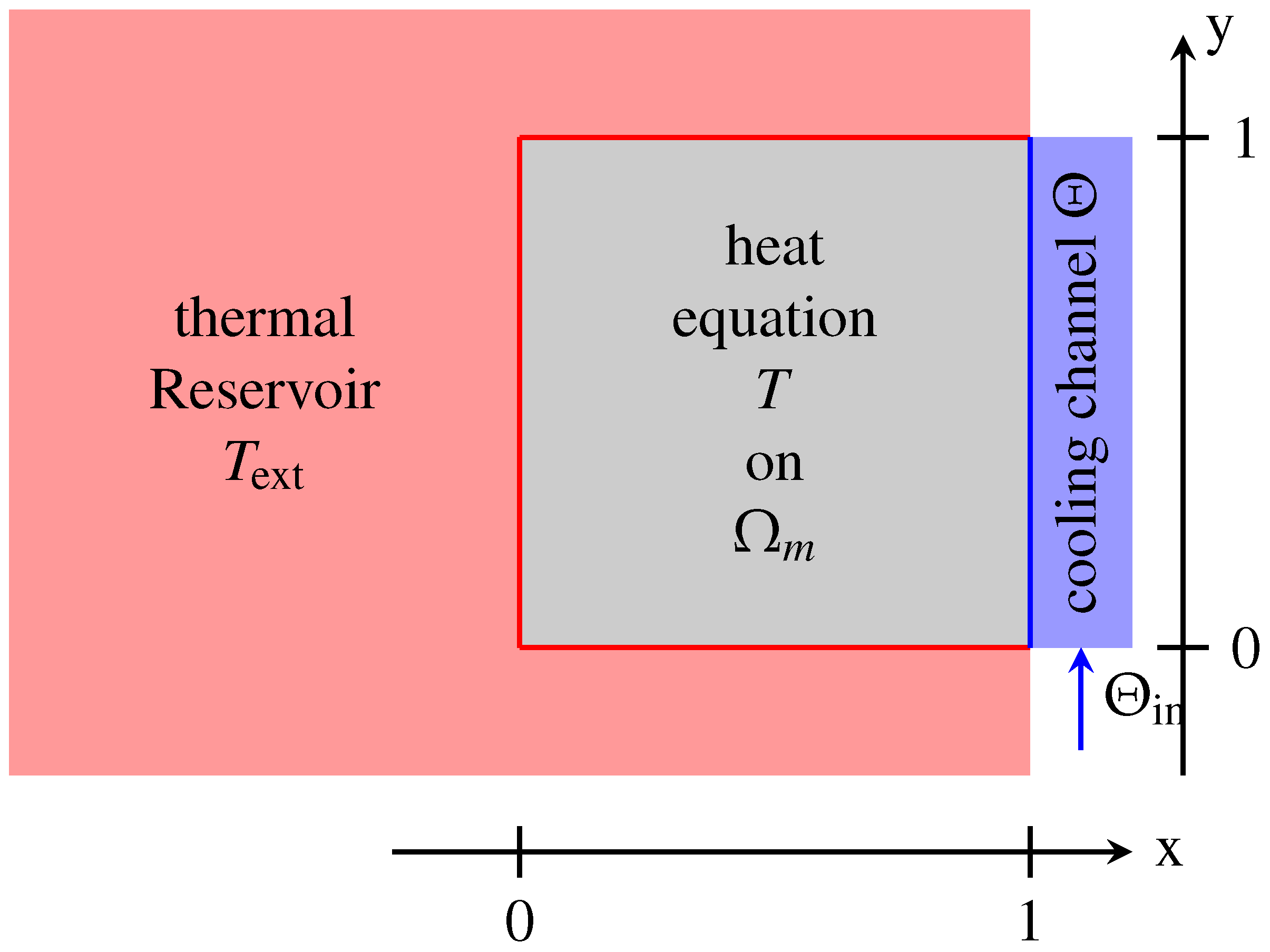
2. The Model System
3. Port-Hamiltonian Formulation
3.1. Heat Equation
3.2. Cooling Channel
3.3. Coupling
4. Finite Difference Discretization
4.1. Heat Equation
4.2. Transport Equation
4.3. Coupling the Discretized Systems
4.4. Discretizing the Coupled System
5. Conclusions and Outlook
Author Contributions
Funding
Data Availability Statement
Conflicts of Interest
References
- Backhaus, J.; Bolten, M.; Doganay, O.T.; Ehrhardt, M.; Engel, B.; Frey, C.; Gottschalk, H.; Günther, M.; Hahn, C.; Jäschke, J.; et al. GivEn—Shape optimization for gas turbines in volatile energy networks. In Mathematical MSO for Power Engineering and Management, Mathematics in Industry; Göttlich, S., Herty, M., Milde, A., Eds.; Springer: Berlin/Heidelberg, Germany, 2021; Volume 34, pp. 71–106. [Google Scholar]
- Han, J.C. Recent studies in turbine blade cooling. Int. J. Rotat. Mach. 2004, 10, 443–457. [Google Scholar]
- Han, J.C.; Dutta, S.; Ekkad, S. Gas Turbine Heat Transfer and Cooling Technology; CRC Press: Boca Raton, FL, USA, 2012. [Google Scholar]
- Kumar, G.; Roelke, R.; Meitner, P. A generalized one dimensional computer code for turbomachinery cooling passage flow calculations. In Proceedings of the 25th Joint Propulsion Conference, Monterey, CA, USA, 12–16 July 1989; p. 2574. [Google Scholar]
- Meitner, P.L. Computer Code for Predicting Coolant Flow and Heat Transfer in Turbomachinery; Technical Report; NASA: Washington, DC, USA, 1990. [Google Scholar]
- Beattie, C.; Mehrmann, V.; Xu, H.; Zwart, H. Linear port-Hamiltonian descriptor systems. Math. Contr. Sign. Syst. 2018, 30, 17. [Google Scholar] [CrossRef] [Green Version]
- Duindam, V.; Macchelli, A.; Stramigioli, S.; Bruyninckx, H. (Eds.) Modeling and Control of Complex Physical Systems—The Port-Hamiltonian Approach; Springer: Berlin/Heidelberg, Germany, 2009. [Google Scholar]
- Jacob, B.; Zwart, H.J. Linear Port-Hamiltonian Systems on Infinite-Dimensional Spaces; Springer Science & Business Media: Berlin/Heidelberg, Germany, 2012; Volume 223. [Google Scholar]
- van der Schaft, A. Port-Hamiltonian systems: An Introductory Survey. In Proceedings of the International Congress of Mathematicians, Madrid, Spain, 22–30 August 2006; Volume III, pp. 1339–1365. [Google Scholar]
- Imam-Lawal, O.R. Adjoint Based Optimisation for Coupled Conjugate Heat Transfer. Ph.D. Thesis, Queen Mary, University of London, London, UK, 2020. [Google Scholar]
- Reyhani, M.R.; Alizadeh, M.; Fathi, A.; Khaledi, H. Turbine blade temperature calculation and life estimation—A sensitivity analysis. Prop. Power Res. 2013, 2, 148–161. [Google Scholar]
- Jäschke, J.; Ehrhardt, M.; Günther, M.; Jacob, B. Discrete port-Hamiltonian coupled heat transfer. In The European Consortium for Mathematics in Industry; Springer: Berlin/Heidelberg, Germany, 2022; pp. 439–445. [Google Scholar]
- Jäschke, J.; Ehrhardt, M.; Günther, M.; Jacob, B. A port-Hamiltonian formulation of coupled heat transfer. Math. Comput. Model. Dyn. Syst. 2022, 28, 78–94. [Google Scholar] [CrossRef]
- van der Schaft, A.; Maschke, B. Hamiltonian formulation of distributed-parameter systems with boundary energy flow. J. Geom. Phys. 2002, 42, 166–194. [Google Scholar] [CrossRef] [Green Version]
- Mehrmann, V.; Morandin, R. Structure-preserving discretization for port-Hamiltonian descriptor systems. In Proceedings of the 58th IEEE Conference on Decision and Control (CDC), Nice, France, 11–13 December 2019; pp. 6863–6868. [Google Scholar]
- Goodman, T.R. Application of integral methods to transient nonlinear heat transfer. Adv. Heat Transf. 1964, 1, 51–122. [Google Scholar]
- Biot, M.A. New methods in heat flow analysis with application to flight structures. J. Aeronaut. Sci. 1957, 24, 857–873. [Google Scholar] [CrossRef] [Green Version]
- Serhani, A.; Haine, G.; Matignon, D. Anisotropic heterogeneous n-D heat equation with boundary control and observation: I. Modeling as port-Hamiltonian system. IFAC-PapersOnLine 2019, 52, 51–56. [Google Scholar] [CrossRef]
- Bird, R.; Stewart, W.; Lightfoot, E. Transport Phenomena, 2nd ed.; John Wiley and Sons: Hoboken, NJ, USA, 2002. [Google Scholar]
- Kurula, M.; Zwart, H. Linear wave systems on n-d spatial domains. Int. J. Control 2015, 88, 1063–1077. [Google Scholar] [CrossRef] [Green Version]
- Le Gorrec, Y.; Zwart, H.; Maschke, B. Dirac structures and boundary control systems associated with skew-symmetric differential operators. SIAM J. Contr. Optim. 2005, 44, 1864–1892. [Google Scholar] [CrossRef] [Green Version]
- Macchelli, A.; van der Schaft, A.; Melchiorri, C. Port-Hamiltonian formulation of infinite dimensional systems I. Modeling. In Proceedings of the 43rd IEEE Conference on Decision and Control (CDC), Nassau, Bahamas, 14–17 December 2004; Volume 4, pp. 3762–3767. [Google Scholar]
- Villegas, J.A. A Port-Hamiltonian Approach to Distributed Parameter Systems. Ph.D. Thesis, University of Twente, Enschede, The Netherlands, 2007. [Google Scholar]
- Cervera, J.; van der Schaft, A.; Baños, A. Interconnection of port-Hamiltonian systems and composition of Dirac structures. Automatica 2007, 43, 212–225. [Google Scholar] [CrossRef] [Green Version]
- Brugnoli, A.; Cardoso-Ribeiro, F.L.; Haine, G.; Kotyczka, P. Partitioned finite element method for structured discretization with mixed boundary conditions. IFAC-PapersOnLine 2020, 53, 7557–7562. [Google Scholar] [CrossRef]
- Cardoso-Ribeiro, F.L.; Matignon, D.; Lefèvre, L. A partitioned finite element method for power-preserving discretization of open systems of conservation laws. IMA J. Math. Contr. Inform. 2020, 38, 493–533. [Google Scholar] [CrossRef]
- Serhani, A.; Matignon, D.; Haine, G. A partitioned finite element method for the structure-preserving discretization of damped infinite-dimensional port-Hamiltonian systems with boundary control. In Geometric Science of Information; Nielsen, F., Barbaresco, F., Eds.; Springer: Cham, Switzerland, 2019; pp. 549–558. [Google Scholar]
- Haine, G.; Matignon, D. Structure-preserving discretization of a coupled heat-wave system, as interconnected port-Hamiltonian systems. In Proceedings of the International Conference on Geometric Science of Information, Paris, France, 21–23 July 2021; Springer: Berlin/Heidelberg, Germany, 2021; pp. 191–199. [Google Scholar]
- Serhani, A.; Haine, G.; Matignon, D. Anisotropic heterogeneous n-D heat equation with boundary control and observation: II. Structure-preserving discretization. IFAC-PapersOnLine 2019, 52, 57–62. [Google Scholar] [CrossRef]
- Brugnoli, A.; Haine, G.; Serhani, A.; Vasseur, X. Numerical approximation of port-Hamiltonian systems for hyperbolic or parabolic PDEs with boundary control. arXiv 2020, arXiv:2007.08326. [Google Scholar] [CrossRef]
- Trenchant, V.; Hu, W.; Ramirez, H.; Le Gorrec, Y. Structure preserving finite differences in polar coordinates for heat and wave equations. IFAC-PapersOnLine 2018, 51, 571–576. [Google Scholar] [CrossRef]
- Gustafsson, B. The convergence rate for difference approximations to mixed initial boundary value problems. Math. Comp. 1975, 29, 396–406. [Google Scholar] [CrossRef]

Publisher’s Note: MDPI stays neutral with regard to jurisdictional claims in published maps and institutional affiliations. |
© 2022 by the authors. Licensee MDPI, Basel, Switzerland. This article is an open access article distributed under the terms and conditions of the Creative Commons Attribution (CC BY) license (https://creativecommons.org/licenses/by/4.0/).
Share and Cite
Jäschke, J.; Ehrhardt, M.; Günther, M.; Jacob, B. A Two-Dimensional port-Hamiltonian Model for Coupled Heat Transfer. Mathematics 2022, 10, 4635. https://doi.org/10.3390/math10244635
Jäschke J, Ehrhardt M, Günther M, Jacob B. A Two-Dimensional port-Hamiltonian Model for Coupled Heat Transfer. Mathematics. 2022; 10(24):4635. https://doi.org/10.3390/math10244635
Chicago/Turabian StyleJäschke, Jens, Matthias Ehrhardt, Michael Günther, and Birgit Jacob. 2022. "A Two-Dimensional port-Hamiltonian Model for Coupled Heat Transfer" Mathematics 10, no. 24: 4635. https://doi.org/10.3390/math10244635