Event-Triggered Optimal Consensus of Heterogeneous Nonlinear Multi-Agent Systems

Abstract

This paper deals with optimal consensus problems of a general heterogeneous nonlinear multi-agent system. A novel filter is proposed for each agent by integrating local gradients with neighboring output information. Using this filter and introducing an appropriate auxiliary variable, the event-triggered control algorithm is obtained within the framework of the prescribed performance control. One of the remarkable properties of the proposed algorithm is that it can save resources by updating control signals only when necessary rather than periodically while achieving optimal consensus. Theoretical and simulation verifications of the algorithm without the Zeno behavior are carefully studied. Instructions are also presented for control parameter selection to keep the residual errors as small as desired.

1. Introduction

Due to its broad application in quadrotors, mobile robots, and network optimization of resource allocation, research on distributed control of multi-agent systems has emerged extensively in the past two decades. Consensus control as a critical distributed feature of networks, where all agents incorporate only local perception to yield a common state, is now a subject of active research [1,2]. Consensus problems for multi-agent systems have yielded many interesting results, ranging from simple integrators to complex nonlinear dynamics and from fixed communication topologies to switched topologies; see [3,4,5,6,7] and references therein. In practice, resource allocation in computer networks and collision avoidance in multi-robot systems can be modeled as distributed optimization problems. Recently, so-called optimal consensus techniques have been proposed, in which established consensus problems and distributed optimization problems are simultaneously solved [8].

By combining set valued stability analysis with convex analysis, continuous-time distributed optimization of convex function sums was realized under a weight-balanced digraph in [9]. By requiring the local cost function to be twice-differentiable, an average consensus strategy was presented such that each agent can asymptotically tend towards the minimum of the global cost function in [10]. This requirement has been removed by [11], where gradient-based distributed algorithms were proposed under both directed and undirected graphs. A common feature of the above works [9,10,11] is that the inherent nonlinear properties and possible disturbances of the agent are not considered. In the presence of external disturbance, an internal-model-based approach was developed to handle dynamic optimization problems in [12]. The disturbances need to satisfy the matching condition, which means the disturbance can only occur in the exact same equation as the control input. These requirements limit the application of the developed methods to a relatively specific class of systems. Recently, by applying three types of disturbance estimators, distributed optimization strategies have been extended to address second-order systems with mismatched and matched disturbances in [13]. In practice, this extension considering only second-order systems and time-dependent perturbations may not be sufficient due to ubiquitous higher-order dynamics and agent state-dependent uncertainty. However, with few exceptions, research on distributed optimal consensus control of more general uncertain higher-order nonlinear systems has received little attention. By constructing an optimal consensus proportional and integral variable, optimal consensus issues of pure-feedback systems have been solved in [14]. Most of the above results rely on the classic time-triggered control paradigm, where the update of the control signal is periodic even when the system is performing well. This can lead to wasted computing and communication resources, as remarked by [15,16].

In this work, we study the optimal consensus problem for nonlinear systems, focusing on saving resources by updating control signals only when necessary rather than periodically. In particular, a more general heterogeneous multi-agent system is investigated where mismatched uncertainties and possibly agent nonidentical dynamical orders are considered. A novel filter for each agent is proposed which combines local gradients with neighboring output information. Subsequently, we complete the optimal consensus control law design by introducing an event-triggered condition and adopting the backstepping design procedure. Using the integrating factor method and the Lyapunov function, we rigorously demonstrate that all agents achieve the approximate optimal consensus under the proposed protocol, and Zeno behavior can be ruled out. The feasibility of implementing our algorithm is demonstrated on a group of single-link manipulators. Compared with the current results, the main contributions are as follows:

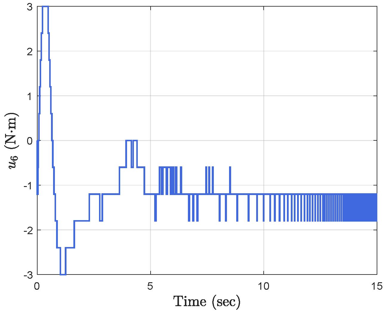
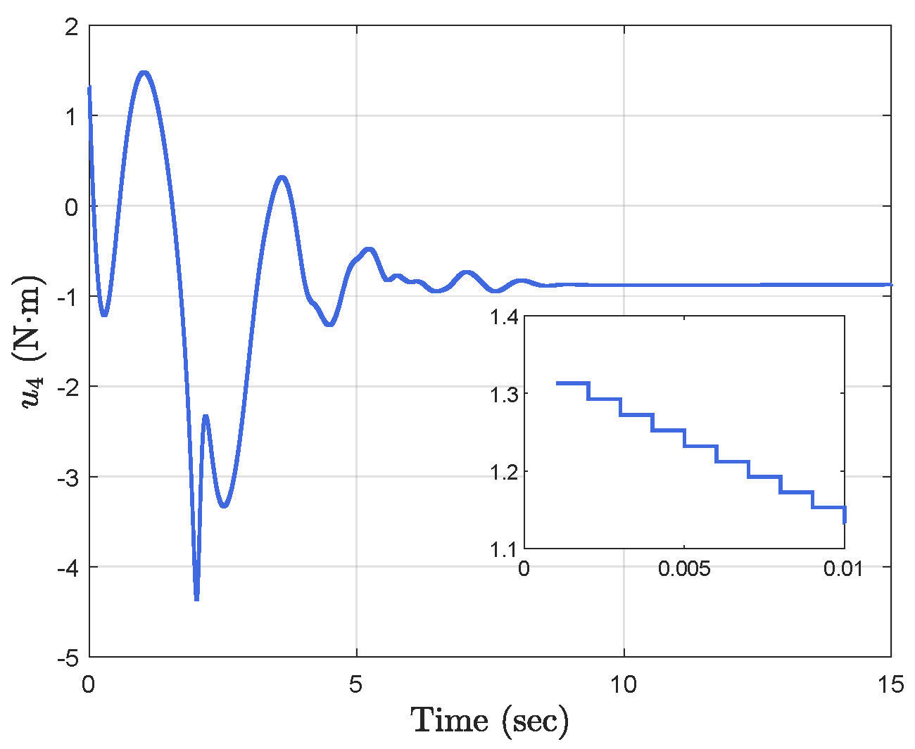
• Different from the classical time-triggered setting, our proposed event-triggered method is able to significantly reduce the unnecessary control input updates while ensuring the approximate optimal consensus.
• In contrast to the study of first- and second-order multi-agent systems, where external disturbances are assumed to be bounded a priori, we study a more general nonlinear dynamics where uncertainty is allowed to grow arbitrarily as the variation of agent states and higher-order heterogeneous dynamics are involved.

The rest of this manuscript is organized as follows. In Section 2, the preliminary knowledge and the optimal consensus problem to be addressed are introduced. Section 3 introduces our novel filter system and event-triggered control algorithm. Section 4 illustrates simulation results of a group of manipulators, while Section 5 draws conclusions and discusses recommendations and outlook.

Notation: Let $0_{\ell }$ and $1_{\ell }$ denote, respectively, the vectors of zeros and ones with length ℓ. For a function $\varphi \left(t\right)$, we say that $\varphi \in {\mathbb{L}}_{\infty }[0,t_f)$ if ${sup}_{0\le t<t_f}\parallel \varphi \left(t\right)\parallel <\infty$.

2. Problem Formulation and Preliminaries

2.1. Preliminaries

Let $\mathcal{G}=\{\mathcal{V},\mathcal{E},\mathcal{A}\}$ represent the graph describing the communication topology, where $\mathcal{V}=\{1,\dots ,n\}$, $\mathcal{E}\subseteq \mathcal{V}\times \mathcal{V}$, and $\mathcal{A}=\left[a_{ij}\right]\in {\mathbb{R}}^{n\times n}$ represent node set, edge set, and adjacency matrix, respectively. An edge $(i,j)\in \mathcal{E}$ indicates that node j can obtain information from node i, node i is the neighbor of node j, and necessarily $(i,j)\in \mathcal{E}$ for an undirected graph. The set of all neighbors of node i is denoted by ${\mathcal{N}}_i$. An undirected graph $\mathcal{G}$ is connected if for each distinct pair of nodes i and j, there is a path from i to j. Let $a_{ij}=1$ if $(j,i)\in \mathcal{E}$ and $a_{ij}=0$ otherwise. The Laplacian matrix $\mathcal{L}=\left[l_{ij}\right]\in {\mathbb{R}}^{n\times n}$ related to $\mathcal{G}$ is defined as $l_{ii}={\sum }_{j\in {\mathcal{N}}_i}{a}_{ij}$ and $l_{ij}=-a_{ij},i\ne j$.

Lemma 1.

([17]). If the undirected graph $\mathcal{G}$ is connected, then there exists a nonsingular matrix $\overline{P}=[p_1,\dots ,p_n]\in {\mathbb{R}}^{n\times n}$ such that

$$\mathcal{L}=\overline{P}\left[\begin{array}{cc}0& 0_{n-1}^{\mathrm{T}}\\ 0_{n-1}& \mathsf{\Lambda }\end{array}\right]{\overline{P}}^{\mathrm{T}}=P\mathsf{\Lambda }{P}^{\mathrm{T}}$$

where $\mathsf{\Lambda }=\mathrm{diag}\{{\lambda }_2,\dots ,{\lambda }_n\}$ with ${\lambda }_{\ell }$ being the positive real eigenvalues of $\mathcal{L}$, $\ell =,2\dots ,n$, $p_{\ell }$ are right eigenvectors of $\mathcal{L}$ associated with ${\lambda }_{\ell }$, $p_1=\frac{1_n}{n}$, and $P=[p_2,\dots ,p_n]$.

2.2. Problem Formulation

Consider a multi-agent system composed of n nonlinear agents. Each agent can be described by the following strict-feedback dynamics [18]:

$$\begin{array}{ccc}\hfill {\dot{x}}_{i,m}& =& f_{i,m}\left({\overline{x}}_{i,m}\right)+{\mathrm{g}}_{i,m}\left({\overline{x}}_{i,m}\right)x_{i,m+1}+d_{i,m}\left(t\right),m=1,\dots ,q_i-1\hfill \\ \hfill {\dot{x}}_{i,q_i}& =& f_{i,q_i}\left({\overline{x}}_{i,q_i}\right)+{\mathrm{g}}_{i,q_i}\left({\overline{x}}_{i,q_i}\right)u_i+d_{i,q_i}\left(t\right)\hfill \end{array}$$

(1)

in which ${\overline{x}}_{i,\ell }={[x_{i,1},\dots ,x_{i,\ell }]}^{\mathrm{T}}\in {\mathbb{R}}^{\ell }$, $\ell =1,\dots ,q_i$, are the state vectors. $y_i=x_{i,1}\in \mathbb{R}$ and $u_i\in \mathbb{R}$ represent the agent’s output and the control input, respectively. ${\mathrm{g}}_{i,\ell }\left({\overline{x}}_{i,\ell }\right),f_{i,\ell }\left({\overline{x}}_{i,\ell }\right):{\mathbb{R}}^{\ell }\to \mathbb{R}$ are nonlinear dynamics functions with unknown analytical expressions. $d_{i,\ell }\left(t\right):[0,\infty )\to \mathbb{R}$ denotes uncertain disturbances. Moreover, $f_{i,\ell }\left({\overline{x}}_{i,\ell }\right)$ and ${\mathrm{g}}_{i,\ell }\left({\overline{x}}_{i,\ell }\right)$ are locally Lipschitz in ${\overline{x}}_{i,\ell }$ and $d_{i,\ell }\left(t\right)$ are piecewise continuous in t. Agent i has a differentiable local cost function $h_i\left(y_i\right):\mathbb{R}\to \mathbb{R}$, which is strongly convex and has a Lipschitz gradient, i.e., there is a constant $M_i>0$ satisfying $|\nabla h_i\left(a\right)-\nabla h_i\left(b\right)|\le M_i$ for all $a,b\in \mathbb{R}.$

Our control goal is to develop a distributed event-triggered controller $u_i$ in (1) such that the agent outputs achieve the approximate optimal consensus, i.e., ${lim\; sup}_{t\to \infty }|y_i\left(t\right)-y^{*}|\le \epsilon$ for all $i=1,\dots ,n$, where $y^{*}$ is the optimal solution of ${min}_{s\in \mathbb{R}}h\left(s\right)={\sum }_{i=1}^n{h}_i\left(s\right)$, and $\epsilon$ is a positive constant that can be made arbitrarily small. In addition, all closed-loop signals are bounded.

To achieve the control goal, we make the following standard assumptions about the agent (1).

Assumption 1.

The communication graph $\mathcal{G}$ is undirected and connected.

Assumption 2.

Unknown $d_{i,\ell }\left(t\right)$, $i=1,\dots ,n$, $\ell =1,\dots ,q_i,$ are bounded. There are strictly positive functions and continuous ${\underline{\mathrm{g}}}_{i,\ell }\left({\overline{x}}_{i,\ell }\right)$ such that ${\underline{\mathrm{g}}}_{i,\ell }\left({\overline{x}}_{i,\ell }\right)\le |{\mathrm{g}}_{i,\ell }\left({\overline{x}}_{i,\ell }\right)|$ for all ${\overline{x}}_{i,\ell }\in {\mathbb{R}}^{\ell }$. Furthermore, the sign of ${\mathrm{g}}_{i,\ell }\left({\overline{x}}_{i,\ell }\right)$ is known.

3. Main Result

3.1. Controller Design

To realize the optimal consensus goal in a distributed manner, we propose a novel third-order filter for agent i utilizing locally available information. Inspired by [5,11], the filter is defined as follows:

$$\begin{array}{ccc}\hfill {\dot{z}}_{i,0}& =& y_i-z_{i,1}\hfill \\ \hfill {\dot{z}}_{i,1}& =& -\alpha \nabla h_i\left(y_i\right)-\beta \sum _{j\in {\mathcal{N}}_i}{a}_{ij}(y_i-y_j)-z_{i,2}\hfill \end{array}$$

(2)

$$\begin{array}{ccc}\hfill {\dot{z}}_{i,2}& =& \alpha \beta \sum _{j\in {\mathcal{N}}_i}{a}_{ij}(y_i-y_j)\hfill \end{array}$$

(3)

where $\alpha >0$ and $\beta >0$ are constants. Furthermore, the auxiliary variable is defined as

$$\begin{array}{ccc}\hfill e_{i,1}& =& z_{i,0}+{\dot{z}}_{i,0}.\hfill \end{array}$$

(4)

Subsequently, a backstepping design method is proposed for each agent by adopting the prescribed performance control technique presented in [19,20]. Specifically, let us define the error variables:

$$e_{i,m}=x_{i,m}-v_{i,m-1},m=2,\dots ,q_i$$

(5)

where $v_{i,m-1}$ are the virtual control. A performance function is introduced as ${\rho }_{i,\ell }\left(t\right)=({\rho }_{i,\ell ,0}-{\rho }_{i,\ell ,\infty })e^{-{\gamma }_{i,\ell }t}+{\rho }_{i,\ell ,\infty },$$\ell =1,\dots ,q_i$, where ${\gamma }_{i,\ell }$, ${\rho }_{i,\ell ,\infty }$, and ${\rho }_{i,\ell ,0}$ are positive constants satisfying ${\rho }_{i,\ell ,\infty }<{\rho }_{i,\ell ,0}$ and $|e_{i,\ell }\left(0\right)|<{\rho }_{i,\ell ,0}$. Without loss of generality, let us assume ${\mathrm{g}}_{i,\ell }\left({\overline{x}}_{i,\ell }\right)>0$. The virtual control laws $v_{i,\ell }$ are proposed as

$$v_{i,\ell }=-{\mathcal{\varpi }}_{i,\ell }{\varphi }_{i,\ell }$$

where ${\mathcal{\varpi }}_{i,\ell }$ are positive gains, ${\varphi }_{i,\ell }=ln\left(\frac{1+{\zeta }_{i,\ell }}{1-{\zeta }_{i,\ell }}\right)$, and ${\zeta }_{i,\ell }=\frac{e_{i,\ell }}{{\rho }_{i,\ell }}$. We propose the event-triggered distributed controller on the ith agent as

$$\begin{array}{ccc}\hfill u_i\left(t\right)& =& v_{i,q_i}\left(t_{i,k}\right),\forall t\in [t_{i,k},t_{i,k+1})\hfill \\ \hfill t_{i,k+1}& =& \inf \{t\in \mathbb{R}:|{\delta }_i\left(t\right)|={\eta }_i\}\hfill \end{array}$$

(6)

where $t_{i,0}=0$, $k=0,1,2,\dots$, ${\delta }_i\left(t\right)=v_{i,q_i}\left(t\right)-v_{i,q_i}\left(t_k\right)$, and ${\eta }_i$ is a positive design parameter.

The strategy behind (3) is to use only relative output measurements and local gradients to generate the reference output. The purpose of introducing (2) is to include an integral term for the tracking error between the output $y_i$ and the reference output $z_{i,1}$ to facilitate stability analysis; similar efforts can also be found in time-triggered control consensus methods [5,14].

3.2. Stability Analysis

Theorem 1.

Consider a group of n uncertain heterogeneous nonlinear agents (1) controlled by the distributed event-triggered controller (6) with the filter (3). Under Assumptions 1 and 2, it holds that each agent can realize the approximate optimal consensus while all signals in the closed-loop system remain bounded. Furthermore, Zeno behavior can be avoided, i.e., there is a constant ${▵}_i^{*}>0$ satisfying $t_{i,k+1}-t_{i,k}\ge {▵}_i^{*}$ for all $k=0,1,2,\dots .$

Proof. 

The state variables $x_{i,1},\dots ,x_{i,q_i}$ of agent i in (1) can be represented by $v_{i,\ell }$, $z_{i,0}$, $z_{i,1}$, $z_{i,2}$ and t as

$$\begin{array}{ccc}{x}_{i,1}\hfill & =\hfill & {\zeta }_{i,1}{\rho }_{i,1}\left(t\right)-z_{i,0}+z_{i,1}\hfill \\ x_{i,m}\hfill & =\hfill & {\zeta }_{i,m}{\rho }_{i,m}\left(t\right)+v_{i,m-1}\left({\zeta }_{i,m-1}\right),m=2,\dots ,q_i.\hfill \end{array}$$

(7)

Note that ${\mathrm{g}}_{i,\ell }$ and $f_{i,\ell }$ are functions of ${\overline{x}}_{i,\ell }$. Therefore, they can be expressed as ${\mathrm{g}}_{i,1}\left(x_{i,1}\right)={\mathrm{g}}_{i,1}({\zeta }_{i,1}{\rho }_{i,1}-z_{i,0}+z_{i,1}),$$f_{i,1}\left(x_{i,1}\right)=f_{i,1}({\zeta }_{i,1}{\rho }_{i,1}-z_{i,0}+z_{i,1}),$${\mathrm{g}}_{i,m}\left({\overline{x}}_{i,m}\right)=$${\mathrm{g}}_{i,m}({\zeta }_{i,1}{\rho }_{i,1}-z_{i,0}+z_{i,1},\dots ,{\zeta }_{i,m}{\rho }_{i,m}+v_{i,m-1}\left({\zeta }_{i,m-1}\right)),$$f_{i,m}\left({\overline{x}}_{i,m}\right)=f_{i,m}({\zeta }_{i,1}{\rho }_{i,1}-z_{i,0}+z_{i,1},$$\dots ,{\zeta }_{i,m}{\rho }_{i,m}+v_{i,m-1}\left({\zeta }_{i,m-1}\right))$. Accordingly, the dynamics of $z_{i,0}$, $z_{i,1}$, and $z_{i,2}$ in (3) can be rewritten as

$$\begin{array}{ccc}\hfill {\dot{z}}_{i,0}& =& {\zeta }_{i,1}{\rho }_{i,1}-z_{i,0}\hfill \\ \hfill {\dot{z}}_{i,1}& =& -\alpha \nabla h_i({\zeta }_{i,1}{\rho }_{i,1}-z_{i,0}+z_{i,1})\hfill \\ & & -\beta \sum _{j\in {\mathcal{N}}_i}{a}_{ij}(({\zeta }_{i,1}{\rho }_{i,1}-z_{i,0}+z_{i,1})-({\zeta }_{j,1}{\rho }_{j,1}-z_{j,0}+z_{j,1}))-z_{i,2}\hfill \\ \hfill {\dot{z}}_{i,2}& =& \alpha \beta \sum _{j\in {\mathcal{N}}_i}{a}_{ij}(({\zeta }_{i,1}{\rho }_{i,1}-z_{i,0}+z_{i,1})-({\zeta }_{j,1}{\rho }_{j,1}-z_{j,0}+z_{j,1})).\hfill \end{array}$$

(8)

Noting from (6) that $|v_{i,q_i}\left(t\right)-u_i\left(t\right)|\le {\eta }_i$, the time derivatives of ${\zeta }_{i,\ell }$, $\ell =1,\dots ,q_i$ are given by

$$\begin{array}{ccc}\hfill {\dot{\zeta }}_{i,1}& =& \frac{1}{{\rho }_{i,1}}(({\dot{z}}_{i,0}+{\dot{x}}_{i,1}-{\dot{z}}_{i,1})-{\zeta }_{i,1}{\dot{\rho }}_{i,1})\hfill \\ & =& \frac{1}{{\rho }_{i,1}}({\dot{z}}_{i,0}-{\dot{z}}_{i,1}-{\zeta }_{i,1}{\dot{\rho }}_{i,1}+f_{i,1}({\zeta }_{i,1}{\rho }_{i,1}-z_{i,0}+z_{i,1})\hfill \\ & & +{\mathrm{g}}_{i,1}({\zeta }_{i,1}{\rho }_{i,1}-z_{i,0}+z_{i,1})({\zeta }_{i,2}{\rho }_{i,2}+v_{i,1}\left({\zeta }_{i,1}\right))+d_{i,1})\hfill \end{array}$$

(9)

$$\begin{array}{ccc}\hfill {\dot{\zeta }}_{i,m}& =& \frac{1}{{\rho }_{i,m}}({\dot{e}}_{i,m}-{\zeta }_{i,m}{\dot{\rho }}_{i,m})\hfill \\ & =& \frac{1}{{\rho }_{i,m}}(f_{i,m}({\zeta }_{i,1}{\rho }_{i,1}-z_{i,0}+z_{i,1},\dots ,{\zeta }_{i,m}{\rho }_{i,m}+v_{i,m-1}\left({\zeta }_{i,m-1}\right))\hfill \\ & & +{\mathrm{g}}_{i,m}({\zeta }_{i,1}{\rho }_{i,1}-z_{i,0}+z_{i,1},\dots ,{\zeta }_{i,m}{\rho }_{i,m}+v_{i,m-1}\left({\zeta }_{i,m-1}\right))\hfill \\ & & \times ({\zeta }_{i,m+1}{\rho }_{i,m+1}+v_{i,m}\left({\zeta }_{i,m}\right))+d_{i,m}+\frac{2{\mathcal{\varpi }}_{i,m-1}}{1-{\zeta }_{i,m-1}^2}{\dot{\zeta }}_{i,m-1}-{\zeta }_{i,m}{\dot{\rho }}_{i,m})\hfill \end{array}$$

(10)

$$\begin{array}{ccc}\hfill {\dot{\zeta }}_{i,q_i}& =& \frac{1}{{\rho }_{i,q_i}}({\dot{e}}_{i,q_i}-{\zeta }_{i,q_i}{\dot{\rho }}_{i,q_i})\hfill \\ & =& \frac{1}{{\rho }_{i,q_i}}(f_{i,q_i}({\zeta }_{i,1}{\rho }_{i,1}-z_{i,0}+z_{i,1},\dots ,{\zeta }_{i,q_i}{\rho }_{i,q_i}+v_{i,q_i-1}\left({\zeta }_{i,q_i-1}\right))\hfill \\ & & +{\mathrm{g}}_{i,q_i}({\zeta }_{i,1}{\rho }_{i,1}-z_{i,0}+z_{i,1},\dots ,{\zeta }_{i,q_i}{\rho }_{i,q_i}+v_{i,q_i-1}\left({\zeta }_{i,q_i-1}\right))v_{i,q_i}\left({\zeta }_{i,q_i}\right)\hfill \\ & & +{\eta }_i+d_{i,q_i}+\frac{2{\mathcal{\varpi }}_{i,q_i-1}}{1-{\zeta }_{i,q_i-1}^2}{\dot{\zeta }}_{i,q_i-1}-{\zeta }_{i,q_i}{\dot{\rho }}_{i,q_i})\hfill \end{array}$$

(11)

where $m=2,\dots ,q_i-1$. Let us define the column vector $\omega =[{\zeta }_{1,1},\dots ,{\zeta }_{1,q_1},\dots ,{\zeta }_{n,1},\dots ,$${\zeta }_{n,q_n},z_{1,0},z_{1,1},z_{1,2},\dots ,z_{n,0},z_{n,1},z_{n,2}{]}^{\mathrm{T}}$ and the nonempty and open set $\mathsf{\Omega }=\{\omega \in {\mathbb{R}}^{q_1+\dots +q_n+3n}|$$-1<{\zeta }_{i,{\ell }_i}<1,i=1,\dots ,n,{\ell }_i=1,\dots ,q_i\}$. Since $-{\rho }_{i,\ell ,0}<e_{i,\ell }\left(0\right)<{\rho }_{i,\ell ,0}$, $\ell =1,\dots ,q_i$, it holds that $\omega \left(0\right)\in \mathsf{\Omega }$. According to (8)–(11), the map f of the closed-loop dynamics $\dot{\omega }=f(\omega ,t)$ over the set $\mathsf{\Omega }$ is piecewise continuous and locally Lipschitz. Therefore, a unique maximal solution $\omega$ of (8)–(11) over $\mathsf{\Omega }$ on $[0,t_f)$ exists, i.e., $\omega \left(t\right)\in \mathsf{\Omega },$$\forall t\in [0,t_f)$.

Now we show that $z_{i,0}\left(t\right)$, $z_{i,1}\left(t\right)$, and $z_{i,2}\left(t\right)$ are bounded on $[0,t_f)$. Applying the integrating factor method to (2) yields

$$z_{i,0}\left(t\right)=e^{-t}{z}_{i,0}\left(0\right)+{\int }_0^t{e}^{-(t-\sigma )}{e}_{i,1}\left(\sigma \right)d\sigma .$$

(12)

It follows from (12) and $e_{i,1}={\rho }_{i,1}{\zeta }_{i,1}$ that $z_{i,0}$ is bounded for any bounded ${\zeta }_{i,1}$. Thus, we can conclude that $z_{i,0}\in {\mathbb{L}}_{\infty }[0,t_f)$. To analyze the boundedness of $z_{i,1}$ and $z_{i,2}$, we define ${\overline{z}}_1=1_n{y}^{*}$ and ${\overline{z}}_2=-\frac{1}{\beta }\nabla H\left({\overline{z}}_1\right)$, where $\nabla H\left(s\right)={[\nabla h\left(s_1\right),\dots ,\nabla h\left(s_n\right)]}^{\mathrm{T}}$ for $s={[s_1,\dots ,s_n]}^{\mathrm{T}}$. Denote the regulation errors as ${\tilde{z}}_1=z_1-{\overline{z}}_1$ and ${\tilde{z}}_2=z_2-{\overline{z}}_2$, which have the following dynamics:

$$\begin{array}{ccc}\hfill {\dot{\tilde{z}}}_1& =& -\beta \mathcal{L}{e}_1-\beta \mathcal{L}{\tilde{z}}_1-\alpha \beta z_2-\alpha \nabla H(e_1-z_0+z_1)\hfill \\ \hfill {\dot{\tilde{z}}}_2& =& \mathcal{L}{z}_1\hfill \end{array}$$

(13)

where $z_{\ell }={[z_{1,\ell },\dots ,z_{n,\ell }]}^{\mathrm{T}}$ with $\ell =0,1,2$ and $e_1={[e_{1,1},\dots ,e_{n,1}]}^{\mathrm{T}}$. Motivated by [14], let us consider the following Lyapunov function

$$V=\frac{1}{2}{r}^{\mathrm{T}}\left[\begin{array}{cc}{I}_n& \vartheta I_n\\ \vartheta I_n& \alpha \beta P{\mathsf{\Lambda }}^{-1}{P}^{\mathrm{T}}+\vartheta \beta I_n\end{array}\right]r$$

(14)

where $r={[{\tilde{z}}_1^{\mathrm{T}},{\tilde{z}}_2^{\mathrm{T}}]}^{\mathrm{T}}$, $\vartheta <\beta$ is positive constant only introduced for stability analysis purposes, and P and $\mathsf{\Lambda }$ are defined in Lemma 1. A straightforward computation similar to [14] gives

$$\dot{V}\le -{\kappa }_{1}V+{\kappa }_2\parallel z_0{\parallel }^2+{\kappa }_3{\parallel e_1\parallel }^2.$$

(15)

Here ${\kappa }_1$, ${\kappa }_2$, and ${\kappa }_3$ are positive constants whose values depend only on $\alpha$, $\beta$, $\vartheta$, the Laplacian matrix $\mathcal{L}$, and the Lipschitz constant $M_i$ for $\nabla h_i$. Since $e_1$ and $z_0$ are bounded on $[0,t_f)$, we can conclude from (15) that V is bounded on $[0,t_f)$. As a result, we have $z_{i,1},z_{i,2}\in {\mathbb{L}}_{\infty }[0,t_f)$. It then follows from (8) that ${\dot{z}}_{i,0},{\dot{z}}_{i,1},{\dot{z}}_{i,2}\in {\mathbb{L}}_{\infty }[0,t_f)$.

Step 1. Consider the Lyapunov function $V_{i,1}=\frac{1}{2}{\varphi }_{i,1}^2$. Differentiating with t and using (9), we have

$$\begin{array}{ccc}\hfill {\dot{V}}_{i,1}& =& \frac{2{\varphi }_{i,1}}{(1-{\zeta }_{i,1}^2){\rho }_{i,1}}({\dot{z}}_{i,0}-{\dot{z}}_{i,1}-{\zeta }_{i,1}{\dot{\rho }}_{i,1}+f_{i,1}({\zeta }_{i,1}{\rho }_{i,1}-z_{i,0}+z_{i,1})\hfill \\ \hfill & & +{\mathrm{g}}_{i,1}({\zeta }_{i,1}{\rho }_{i,1}-z_{i,0}+z_{i,1})({\zeta }_{i,2}{\rho }_{i,2}-{\mathcal{\varpi }}_{i,1}{\varphi }_{i,1})+d_{i,1}).\hfill \end{array}$$

(16)

Since ${\zeta }_{i,\ell }\in (-1,1)$, $\ell =1,\dots ,q_i$ for all $[0,t_f)$, $z_{i,0},z_{i,1},{\dot{z}}_{i,0},{\dot{z}}_{i,1}\in {\mathbb{L}}_{\infty }[0,t_f)$, and ${\rho }_{i,1}$, ${\dot{\rho }}_{i,1}$, ${\rho }_{i,2}$ and $d_i$ are always bounded, considering the continuity of $f_{i,1}$ and ${\mathrm{g}}_{i,1}$ and applying the extreme value theorem and Assumption 2 can obtain that $|{\dot{z}}_{i,0}-{\dot{z}}_{i,1}-{\zeta }_{i,1}{\dot{\rho }}_{i,1}+f_{i,1}({\zeta }_{i,1}{\rho }_{i,1}-z_{i,0}+z_{i,1})+{\mathrm{g}}_{i,1}({\zeta }_{i,1}{\rho }_{i,1}-z_{i,0}+z_{i,1}){\zeta }_{i,2}{\rho }_{i,2}+d_{i,1}|\le {\overline{f}}_{i,1}^{*}$, ${\underline{\mathrm{g}}}_{i,1}^{*}\le {\mathrm{g}}_{i,1}({\zeta }_{i,1}{\rho }_{i,1}-z_{i,0}+z_{i,1})$ for positive constants ${\overline{f}}_{i,1}^{*}$ and ${\underline{\mathrm{g}}}_{i,1}^{*}$ for all $t\in [0,t_f)$. This together with the fact that $\frac{2}{(1-{\zeta }_{i,1}^2){\rho }_{i,1}}>0$ gives:

$${\dot{V}}_{i,1}\le \frac{2}{(1-{\zeta }_{i,1}^2){\rho }_{i,1}}(-{\underline{\mathrm{g}}}_{i,1}^{*}{\mathcal{\varpi }}_{i,1}{\varphi }_{i,1}^2+{\overline{f}}_{i,1}^{*}|{\varphi }_{i,1}|),\forall t\in [0,t_f).$$

Therefore, ${\dot{V}}_{i,1}\left(t\right)<0$ provided $|{\varphi }_{i,1}|>\frac{{\overline{f}}_{i,1}^{*}}{{\underline{\mathrm{g}}}_{i,1}^{*}{\mathcal{\varpi }}_{i,1}}$, $\forall t\in [0,t_f)$. We obtain

$$|{\varphi }_{i,1}\left(t\right)|\le {\varphi }_{i,1}^{*}=max\{|{\varphi }_{i,1}\left(0\right)|,\frac{{\overline{f}}_{i,1}^{*}}{{\underline{\mathrm{g}}}_{i,1}^{*}{\mathcal{\varpi }}_{i,1}}\},\forall t\in [0,t_f).$$

(17)

Hence, the virtual control $v_{i,1}\left({\zeta }_{i,1}\left(t\right)\right)$ is bounded on $[0,t_f)$. By taking the inverse logarithmic function in ${\varphi }_{i,1}$, we obtain

$$-1<{\underline{\zeta }}_{i,1}\le {\zeta }_{i,1}\left(t\right)\le {\overline{\zeta }}_{i,1}<1,\forall t\in [0,t_f)$$

(18)

where ${\underline{\zeta }}_{i,1}=(e^{-{\varphi }_{i,1}^{*}}-1)/(e^{-{\varphi }_{i,1}^{*}}+1)$ and ${\overline{\zeta }}_{i,1}=(e^{{\varphi }_{i,1}^{*}}-1)/(e^{{\varphi }_{i,1}^{*}}+1)$. In addition, noting (9) and ${\dot{v}}_{i,1}\left(t\right)=\frac{-2{\mathcal{\varpi }}_{i,1}}{1-{\zeta }_{i,1}^2}{\dot{\zeta }}_{i,1}$, we have ${\dot{\zeta }}_{i,1}\left(t\right)$ and $v_{i,1}\left(t\right)$ are bounded on $[0,t_f)$.

Step m ($m=2,\dots ,q_i$). Applying the method from step 1 recursively to the remaining steps and selecting $V_{i,m}=\frac{1}{2}{\varphi }_{i,m}^2$, we can obtain

$${\dot{V}}_{i,m}\le \frac{2}{(1-{\zeta }_{i,m}^2){\rho }_{i,m}}(-{\underline{\mathrm{g}}}_{i,m}^{*}{\mathcal{\varpi }}_{i,m}{\varphi }_{i,m}^2+{\overline{f}}_{i,m}^{*}|{\varphi }_{i,m}|),\forall t\in [0,t_f)$$

(19)

where ${\overline{f}}_{i,m}^{*}>0$ and ${\underline{\mathrm{g}}}_{i,m}^{*}>0$ are constants satisfying:

$$\begin{array}{c}{\underline{\mathrm{g}}}_{i,m}^{*}\le {\mathrm{g}}_{i,m}({\zeta }_{i,1}{\rho }_{i,1}-z_{i,0}+z_{i,1},\dots ,{\zeta }_{i,m}{\rho }_{i,m}+v_{i,m-1}\left({\zeta }_{i,m-1}\right)),m=2,\dots ,q_i\hfill \\ |f_{i,\ell }({\zeta }_{i,1}{\rho }_{i,1}-z_{i,0}+z_{i,1},\dots ,{\zeta }_{i,\ell }{\rho }_{i,\ell }+v_{i,\ell -1}\left({\zeta }_{i,\ell -1}\right))+d_{i,\ell }+\frac{2{\mathcal{\varpi }}_{i,\ell -1}}{1-{\zeta }_{i,\ell -1}^2}{\dot{\zeta }}_{i,\ell -1}-{\zeta }_{i,\ell }{\dot{\rho }}_{i,\ell }\\ \hfill +{\mathrm{g}}_{i,\ell }({\zeta }_{i,1}{\rho }_{i,1}-z_{i,0}+z_{i,1},\dots ,{\zeta }_{i,\ell }{\rho }_{i,\ell }+v_{i,\ell -1}\left({\zeta }_{i,\ell -1}\right)){\zeta }_{i,\ell +1}{\rho }_{i,\ell +1}|\le {\overline{f}}_{i,\ell }^{*},\ell =2,\dots ,q_i-1\end{array}$$

$$\begin{array}{c}|f_{i,q_i}({\zeta }_{i,1}{\rho }_{i,1}-z_{i,0}+z_{i,1},\dots ,{\zeta }_{i,q_i}{\rho }_{i,q_i}+v_{i,q_i-1}\left({\zeta }_{i,q_i-1}\right))\hfill \\ \hfill \hspace{1em}\hspace{1em}\hspace{1em}\hspace{1em}\hspace{1em}\hspace{1em}\hspace{1em}\hspace{1em}\hspace{1em}\hspace{1em}\hspace{1em}\hspace{1em}\hspace{1em}\hspace{1em}+{\eta }_i+d_{i,q_i}+\frac{2{\mathcal{\varpi }}_{i,q_i-1}}{1-{\zeta }_{i,q_i-1}^2}{\dot{\zeta }}_{i,q_i-1}-{\zeta }_{i,q_i}{\dot{\rho }}_{i,q_i}|\le {\overline{f}}_{i,q_i}^{*}.\end{array}$$

It then follows from (19) that

$$|{\varphi }_{i,m}\left(t\right)|\le {\varphi }_{i,m}^{*}=max\{|{\varphi }_{i,m}\left(0\right)|,\frac{{\overline{f}}_{i,m}^{*}}{{\underline{\mathrm{g}}}_{i,m}^{*}{\mathcal{\varpi }}_{i,m}}\},\forall t\in [0,t_f).$$

(20)

Consequently, the virtual control $v_{i,m}\left({\zeta }_{i,1}\left(t\right)\right)$ is bounded on $[0,t_f)$ and ${\zeta }_{i,m}$ satisfies

$$-1<{\underline{\zeta }}_{i,m}\le {\zeta }_{i,m}\left(t\right)\le {\overline{\zeta }}_{i,m}<1,\forall t\in [0,t_f)$$

(21)

where ${\underline{\zeta }}_{i,m}=(e^{-{\varphi }_{i,m}^{*}}-1)/(e^{-{\varphi }_{i,m}^{*}}+1)$ and ${\overline{\zeta }}_{i,m}=(e^{{\varphi }_{i,m}^{*}}-1)/(e^{{\varphi }_{i,m}^{*}}+1)$. In addition, noting (10) and (11) and ${\dot{v}}_{i,m}\left(t\right)=\frac{-2{\mathcal{\varpi }}_{i,m}}{1-{\zeta }_{i,m}^2}{\dot{\zeta }}_{i,m}$, we have ${\dot{\zeta }}_{i,m}\left(t\right)$, $v_{i,m}\left(t\right)$, and ${\dot{v}}_{i,m}\left(t\right)$ are bounded on $[0,t_f)$. Notice by (18), (21), and $z_{i,0},z_{i,1},z_{i,2}\in {\mathbb{L}}_{\infty }[0,t_f)$ that $\omega \left(t\right)\in {\mathsf{\Omega }}^{*}$ for all $t\in [0,t_f)$, where ${\mathsf{\Omega }}^{*}$ is a nonempty and compact subset of $\mathsf{\Omega }$. Therefore, the solution is global, i.e., $t_f=\infty$.

Next, we show that all agents can realize the approximate optimal consensus. Invoking (12) and (18) leads to

$$\begin{array}{ccc}\hfill |z_{i,0}\left(t\right)|& =& e^{-t}|z_{i,0}\left(0\right)|+{\int }_0^t{e}^{-(t-\sigma )}|e_{i,1}\left(\sigma \right)|d\sigma \hfill \\ & \le & e^{-t}|z_{i,0}\left(0\right)|+{\int }_0^t{e}^{-(t-\sigma )}{\rho }_{i,1}\left(\sigma \right)d\sigma .\hfill \end{array}$$

This indicates that

$$|z_{i,0}\left(t\right)|\le \left\{\begin{array}{cc}{e}^{-t}|z_{i,0}\left(0\right)|+({\rho }_{i,1,0}-{\rho }_{i,1,\infty })t{e}^{-t}+{\rho }_{i,1,\infty }(1-e^{-t}),\hfill & \mathrm{if}{\gamma }_{i,1}=1\hfill \\ e^{-t}|z_{i,0}\left(0\right)|+\frac{{\rho }_{i,1,0}-{\rho }_{i,1,\infty }}{1-{\gamma }_{i,1}}(e^{-{\gamma }_{i,1}t}-e^{-t})+{\rho }_{i,1,\infty }(1-e^{-t}),\hfill & \mathrm{else}\hfill \end{array}\right.$$

(22)

In addition, by (15), we further have

$$\begin{array}{ccc}\hfill V\left(t\right)& =& e^{-{\kappa }_{1}t}V\left(0\right)+{\int }_0^t{e}^{-{\kappa }_1(t-\sigma )}({\kappa }_2\parallel z_0{\left(\sigma \right)\parallel }^2+{\kappa }_3\parallel e_1\left(\sigma \right){\parallel }^2)d\sigma .\hfill \end{array}$$

(23)

Noting that $|e_{i,1}\left(t\right)|\le ({\rho }_{i,\ell ,0}-{\rho }_{i,\ell ,\infty })e^{-{\gamma }_{i,\ell }t}+{\rho }_{i,\ell ,\infty }$ and (22), we can conclude $e_1$ and $z_0$ exponentially converge to the compact set ${\mathsf{\Psi }}_0=\{z_0\in {\mathbb{R}}^n|\parallel z_0{\parallel }^2\le {\sum }_{i=1}^n{\rho }_{i,1,\infty }^2\}$ and ${\mathsf{\Psi }}_1=\{e_1\in {\mathbb{R}}^n|\parallel e_1{\parallel }^2\le {\sum }_{i=1}^n{\rho }_{i,1,\infty }^2\}$, respectively. Furthermore, we can conclude from (23) that V also converges exponentially to the compact set ${\mathsf{\Psi }}_2=\{V\in \mathbb{R}|V\le \frac{({\kappa }_2+{\kappa }_3){\sum }_{i=1}^n{\rho }_{i,1,\infty }^2}{{\kappa }_1}\}$. which can be kept arbitrarily small by reducing ${\rho }_{i,1,\infty }$. By the definition of V in (14), ${\tilde{z}}_{i,1}$ and ${\tilde{z}}_{i,2}$ tend towards an arbitrarily small neighborhood around zero. Recalling ${\overline{z}}_1=1_n{y}^{*}$ and ${\tilde{z}}_1=z_1-{\overline{z}}_1$, we can conclude that all agents can reach the approximate optimal consensus, i.e., ${lim\; sup}_{t\to \infty }|y_i\left(t\right)-y^{*}|\le \epsilon$ for all $i=1,\dots ,n$, where $\epsilon$ is a positive constant that can be made arbitrarily small by decreasing ${\rho }_{i,1,\infty }$.

We are now in a position to show that there is a constant ${▵}_i^{*}>0$ such that $t_{i,k+1}-t_{i,k}\ge {▵}_i^{*}$ for all $k=0,1,2\dots$. Recalling ${\delta }_i\left(t\right)=v_{i,q_i}\left(t\right)-v_{i,q_i}\left(t_k\right)$ for all $t\in [t_{i,k},t_{i,k+1})$, we have $|{\dot{\delta }}_i\left(t\right)|=|{\dot{v}}_{i,q_i}\left(t\right)|$. Since ${\dot{v}}_{i,q_i}$ is bounded, there exists a positive constant ${\varsigma }_i$ such that $|{\dot{\delta }}_i\left(t\right)|\le {\varsigma }_i$. Considering that ${\delta }_i\left(t_{i,k}\right)=0$ and ${lim}_{t\to t_{i,k+1}}{\delta }_i\left(t\right)={\eta }_i$, it can be inferred that there must exist a positive constant ${▵}_i^{*}=\frac{{\eta }_i}{{\varsigma }_i}$ satisfying $t_{i,k+1}-t_{i,k}\ge {▵}_i^{*}$. Thus, we have completed proving that the resulting control input updates are free from Zeno behavior. □

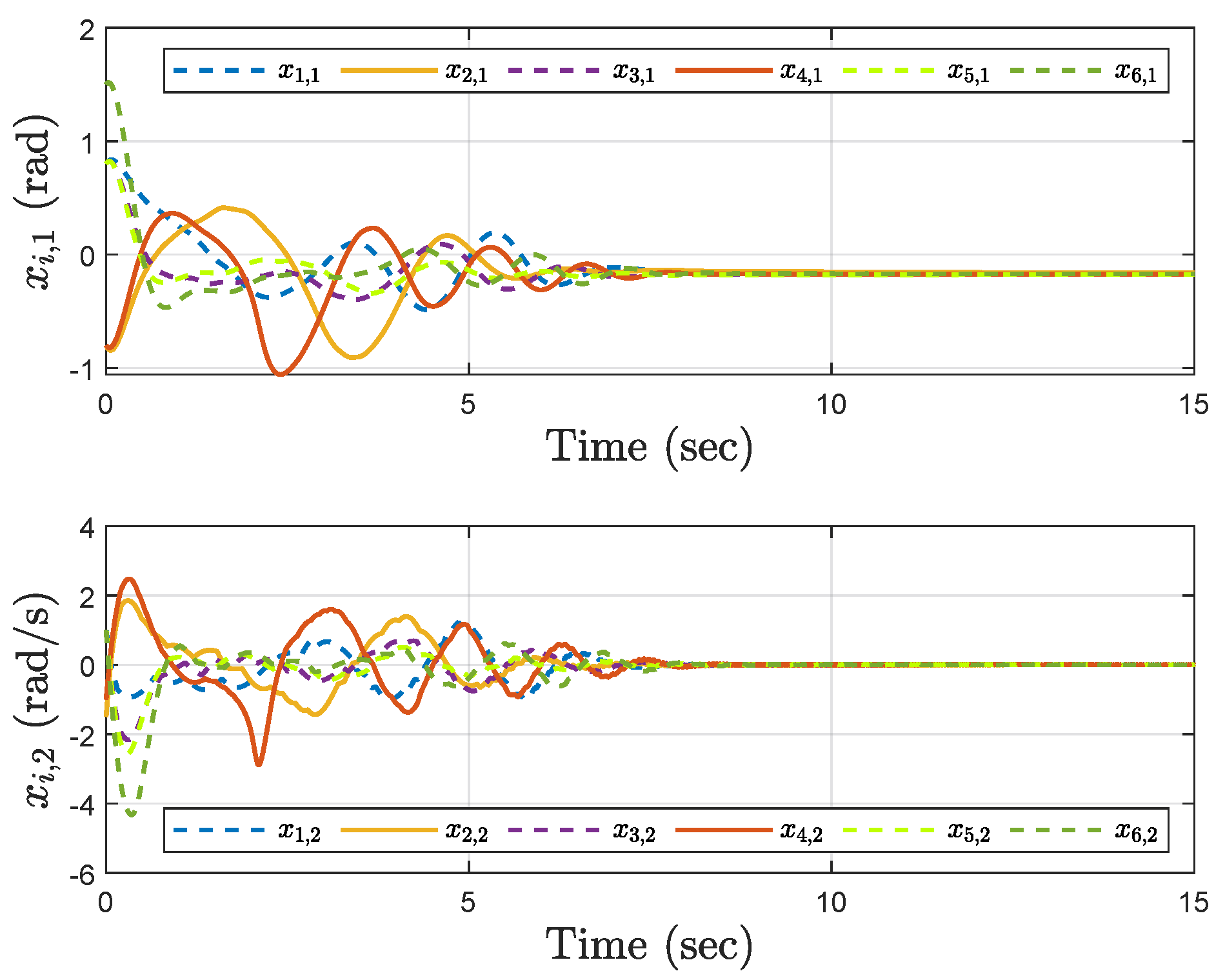
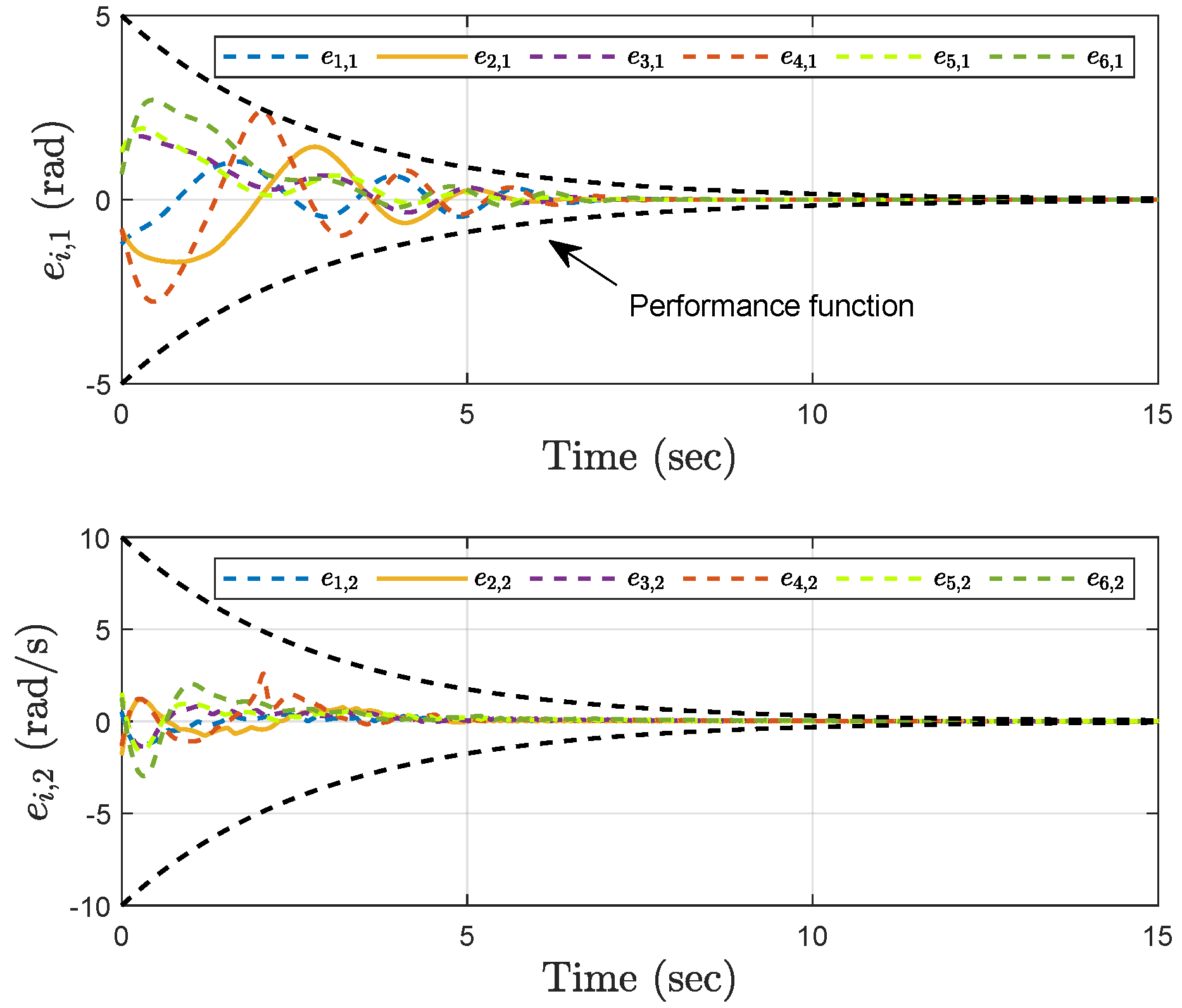
4. Simulation Results

We illustrate the application of our method with a numerical example involving six single-link robotic manipulators, as shown in Figure 1. The ith manipulator is described by the following dynamics:

$$\begin{array}{ccc}{\dot{x}}_{i,1}& =\hfill & x_{i,2}\hfill \\ {\dot{x}}_{i,2}& =\hfill & \frac{1}{J_i}(u_i-{\xi }_i{x}_{i,2}-M_i\mathrm{g}{\chi }_{i}sin\left(x_{i,1}\right)),i=1,\dots ,6\hfill \end{array}$$

(24)

where ${\overline{x}}_i={[x_{i,1},x_{i,2}]}^{\mathrm{T}}$ with $x_{i,1}\in \mathbb{R}$ and $x_{i,2}\in \mathbb{R}$ representing the angle of the link and the angular velocity, respectively. $u_i\in \mathbb{R}$ denotes the control torque. $\mathrm{g}$, $J_i$, ${\xi }_i$, $M_i$, and ${\chi }_i$ are uncertain physical parameters whose definition can be found in [21]. The communication topology between the manipulators is shown in Figure 2. The parameters of the manipulator models are: $\mathrm{g}=9.81$, $J_i=0.1+0.03i$, ${\xi }_i=0.2+0.01i,$$M_i=0.5+0.02i,$ and ${\chi }_i=0.3+0.15i$. The local cost functions $h_i$ are chosen as:

$$\begin{array}{c}{h}_1\left(x_{1,1}\right)={(x_{1,1}-0.5)}^2,h_2\left(x_{2,1}\right)=x_{2,1}^2+e^{0.1x_{2,1}},h_3\left(x_{3,1}\right)={(x_{3,1}+0.1)}^2,\\ h_4\left(x_{4,1}\right)=1.5x_{4,1}^2+2x_{4,1}+1,h_5\left(x_{5,1}\right)=1.3x_{5,1}^2-1,h_6\left(x_{6,1}\right)=x_{6,1}^2-x_{6,1}+4.\end{array}$$

The initial configurations of the manipulators are ${\overline{x}}_1\left(0\right)={[0.8,1]}^{\mathrm{T}}$, ${\overline{x}}_2\left(0\right)={[-0.8,-1.5]}^{\mathrm{T}}$, ${\overline{x}}_3\left(0\right)={[0.8,1]}^{\mathrm{T}}$, ${\overline{x}}_4\left(0\right)={[-0.8,-1]}^{\mathrm{T}}$, ${\overline{x}}_5\left(0\right)={[0.8,1]}^{\mathrm{T}}$, and ${\overline{x}}_6\left(0\right)={[1.5,1]}^{\mathrm{T}}$. The filter (2) and (3) and controller (6) are implemented with the parameters ${\mathcal{\varpi }}_{i,1}=1$, ${\mathcal{\varpi }}_{i,2}=5$, ${\eta }_i=0.6$, $\alpha =1$, and $\beta =1$. The performance functions are set to ${\rho }_{i,1}\left(t\right)=(5-0.01)e^{-0.35t}+0.01$ and ${\rho }_{i,2}\left(t\right)=(10-0.01)e^{-0.35t}+0.01$.

Simulation results show the performance of the proposed event-triggered controller in Figure 3, Figure 4, Figure 5, Figure 6, Figure 7, Figure 8, Figure 9 and Figure 10. The manipulator angles and velocities are exhibited in Figure 3, from which a satisfactory consensus has been reached. Furthermore, the minimizer of the global cost function $h\left(y\right)={\sum }_{i=1}^6{h}_i\left(y\right)$ is $y^{*}=-0.022$. Figure 3 also reveals that each manipulator angle converges to $y^{*}$, although only the neighboring output information and local gradients are available. In addition, as the optimal consensus approaches, the velocity of the manipulator decreases and converges to zero. The evolution of the errors $e_{i,1}$ and $e_{i,2}$ is shown in Figure 4 along with their corresponding performance functions. Clearly, $e_{i,1}$ and $e_{i,2}$ always fulfill the predefined performance specification, as manifested by the theoretical analysis, despite the presence of event-triggered control inputs. The required control input of each manipulator is pictured in Figure 5, Figure 6, Figure 7, Figure 8, Figure 9 and Figure 10, respectively. We can observe from Figure 5, Figure 6, Figure 7, Figure 8, Figure 9 and Figure 10 that the value of the manipulator control is updated aperiodically, only when certain conditions violate the specification (refer to (6)). If the condition is not violated, the value of the control will remain as the value of the last updated controller. To show the advantages of the proposed event-triggered method, a comparative simulation is also carried out, in which the control signal update is periodic and the period is chosen as 1 ms. Simulation results show the performance of the time-triggered controller in Figure 11, Figure 12, Figure 13, Figure 14, Figure 15, Figure 16 and Figure 17. Furthermore,

Table 1. The number of updates for controls under event-triggered controllers and periodic time-triggered controllers.

	Manipulator 1	Manipulator 2	Manipulator 3
Event-triggered control	1130	716	630
Periodic time-triggered control	15,000	15,000	15,000
	Manipulator 4	Manipulator 5	Manipulator 6
Event-triggered control	949	551	171
Periodic time-triggered control	15,000	15,000	15,000

summarizes the corresponding update times of the five manipulator control signals under the event-triggered controller and the time-triggered controller. These results confirm that our event-triggered control method can achieve the approximate optimal consensus similar to the time-triggered controller, while greatly reducing the number of control signal updates and saving computation and communication resources.

5. Conclusions

A novel event-triggered control framework has been presented in this work to realize optimal consensus control of nonlinear agents. It saves resources without sacrificing consensus convergence by proposing new filters and introducing event-triggered rules to reduce unnecessary control signal updates. Furthermore, we confirmed the Zeno-free nature of the method by demonstrating that there is a positive lower bound between two consecutive updates of the control input. Simulation results of single-link manipulators validated our theoretical finding. Some open questions are worthy of further investigation, including the extension of the current results to more general switching topologies and robust analysis of communication delays.

References

1. Psillakis, H.E. Consensus in networks of agents with unknown high-frequency gain signs and switching topology. IEEE Trans. Autom. Control 2017, 62, 3993–3998. [Google Scholar] [CrossRef]
2. Abdessameud, A.; Tayebi, A. Distributed consensus algorithms for a class of high-order multi-agent systems on directed graphs. IEEE Trans. Autom. Control 2018, 63, 3464–3470. [Google Scholar] [CrossRef]
3. Ren, W. On consensus algorithms for double-integrator dynamics. IEEE Trans. Autom. Control 2008, 53, 1503–1509. [Google Scholar] [CrossRef]
4. Wang, G. Distributed control of higher-order nonlinear multi-agent systems with unknown non-identical control directions under general directed graphs. Automatica 2019, 110, 108559. [Google Scholar] [CrossRef]
5. Wang, G. Consensus control in heterogeneous nonlinear multiagent systems with position feedback and switching topologies. IEEE Trans. Netw. Sci. Eng. 2022, 9, 3546–3557. [Google Scholar] [CrossRef]
6. Wang, Q.; Psillakis, H.E.; Sun, C. Cooperative control of multiple agents with unknown high-frequency gain signs under unbalanced and switching topologies. IEEE Trans. Autom. Control 2019, 64, 2495–2501. [Google Scholar] [CrossRef] [Green Version]
7. Mei, J.; Ren, W.; Chen, J. Distributed consensus of second-order multi-agent systems with heterogeneous unknown inertias and control gains under a directed graph. IEEE Trans. Autom. Control 2016, 61, 2019–2034. [Google Scholar] [CrossRef]
8. Yang, F.; Yu, Z.; Huang, D.; Jiang, H. Distributed optimization for second-order multi-agent systems over directed networks. Mathematics 2022, 10, 3803. [Google Scholar] [CrossRef]
9. Gharesifard, B.; Cortés, J. Distributed continuous-time convex optimization on weight-balanced digraphs. IEEE Trans. Autom. Control 2014, 59, 781–786. [Google Scholar] [CrossRef] [Green Version]
10. Zanella, F.; Varagnolo, D.; Cenedese, A.; Pillonetto, G.; Schenato, L. Newton-Raphson consensus for distributed convex optimization. In Proceedings of the 2011 50th IEEE Conference on Decision and Control and European Control Conference, Orlando, FL, USA, 12–15 December 2011; pp. 5917–5922. [Google Scholar]
11. Kia, S.S.; Cortés, J.; Martínez, S. Distributed convex optimization via continuous-time coordination algorithms with discrete-time communication. Automatica 2015, 55, 254–264. [Google Scholar] [CrossRef]
12. Wang, X.; Yi, P.; Hong, Y. Dynamic optimization for multi-agent systems with external disturbances. Control Theory Technol. 2014, 12, 132–138. [Google Scholar] [CrossRef]
13. Wang, X.; Li, S.; Wang, G. Distributed optimization for disturbed second-order multiagent systems based on active antidisturbance control. IEEE Trans. Neural Netw. Learn. Syst. 2019, 31, 2104–2117. [Google Scholar] [CrossRef] [PubMed]
14. Gkesoulis, A.K.; Psillakis, H.E.; Lagos, A.R. Optimal consensus via OCPI regulation for unknown pure-feedback agents with disturbances and state-delays. IEEE Trans. Autom. Control 2022, 67, 4338–4345. [Google Scholar] [CrossRef]
15. Xing, L.; Wen, C.; Liu, Z.; Su, H.; Cai, J. Event-triggered adaptive control for a class of uncertain nonlinear systems. IEEE Trans. Autom. Control 2017, 62, 2071–2076. [Google Scholar] [CrossRef]
16. Zhuang, J.; Li, Z.; Hou, Z.; Yang, C. Event-triggered consensus control of nonlinear strict feedback multi-agent systems. Mathematics 2022, 10, 1596. [Google Scholar] [CrossRef]
17. Bai, H.; Arcak, M. Instability mechanisms in cooperative control. IEEE Trans. Autom. Control 2009, 55, 258–263. [Google Scholar] [CrossRef]
18. Wang, G.; Wang, C.; Ding, Z.; Ji, Y. Distributed consensus of nonlinear multi-agent systems with mismatched uncertainties and unknown high-frequency gains. IEEE Trans. Circuits Syst. II Express Briefs 2021, 68, 938–942. [Google Scholar] [CrossRef]
19. Bechlioulis, C.P.; Rovithakis, G.A. A low-complexity global approximation-free control scheme with prescribed performance for unknown pure feedback systems. Automatica 2014, 50, 1217–1226. [Google Scholar] [CrossRef]
20. Bechlioulis, C.P.; Rovithakis, G.A. Robust adaptive control of feedback linearizable MIMO nonlinear systems with prescribed performance. IEEE Trans. Autom. Control 2008, 53, 2090–2099. [Google Scholar] [CrossRef]
21. Spong, M.W.; Hutchinson, S.; Vidyasagar, M. Robot Modeling and Control; John Wiley & Sons: Hoboken, NJ, USA, 2020. [Google Scholar]
Figure 1. Single-link manipulator.
Mathematics 10 04622 g001
Figure 2. Communication topology.
Mathematics 10 04622 g002
Figure 3. Trajectories of the angles x i , 1 and the velocities x i , 2 under the event−triggered control.
Mathematics 10 04622 g003
Figure 4. Trajectories of the errors e i , 1 and e i , 2 under the event−triggered control.
Mathematics 10 04622 g004
Figure 5. Event−triggered control input u 1 .
Mathematics 10 04622 g005
Figure 6. Event−triggered control input u 2 .
Mathematics 10 04622 g006
Figure 7. Event−triggered control input u 3 .
Mathematics 10 04622 g007
Figure 8. Event−triggered control input u 4 .
Mathematics 10 04622 g008
Figure 9. Event−triggered control input u 5 .
Mathematics 10 04622 g009
Figure 10. Event−triggered control input u 6 .
Mathematics 10 04622 g010
Figure 11. Trajectories of the angles x i , 1 and the velocities x i , 2 under the time−triggered control.
Mathematics 10 04622 g011
Figure 12. Time−triggered control input u 1 .
Mathematics 10 04622 g012
Figure 13. Time−triggered control input u 2 .
Mathematics 10 04622 g013
Figure 14. Time−triggered control input u 3 .
Mathematics 10 04622 g014
Figure 15. Time−triggered control input u 4 .
Mathematics 10 04622 g015
Figure 16. Time−triggered control input u 5 .
Mathematics 10 04622 g016
Figure 17. Time−triggered control input u 6 .
Mathematics 10 04622 g017