Article

TwoViewDensityNet: Two-View Mammographic Breast Density Classification Based on Deep Convolutional Neural Network

1
Department of Computer Science, College of Computer and Information Sciences, King Saud University, Riyadh 11451, Saudi Arabia
2
Department of Software Engineering, College of Computer and Information Sciences, King Saud University, Riyadh 11543, Saudi Arabia
3
Department of Radiology, College of Medicine, King Khalid University Hospital, King Saud University, Riyadh 12372, Saudi Arabia
*
Author to whom correspondence should be addressed.
Mathematics 2022, 10(23), 4610; https://doi.org/10.3390/math10234610
Submission received: 27 October 2022 / Revised: 21 November 2022 / Accepted: 24 November 2022 / Published: 5 December 2022

Abstract

:
Dense breast tissue is a significant factor that increases the risk of breast cancer. Current mammographic density classification approaches are unable to provide enough classification accuracy. However, it remains a difficult problem to classify breast density. This paper proposes TwoViewDensityNet, an end-to-end deep learning-based method for mammographic breast density classification. The craniocaudal (CC) and mediolateral oblique (MLO) views of screening mammography provide two different views of each breast. As the two views are complementary, and dual-view-based methods have proven efficient, we use two views for breast classification. The loss function plays a key role in training a deep model; we employ the focal loss function because it focuses on learning hard cases. The method was thoroughly evaluated on two public datasets using 5-fold cross-validation, and it achieved an overall performance (F-score of 98.63%, AUC of 99.51%, accuracy of 95.83%) on DDSM and (F-score of 97.14%, AUC of 97.44%, accuracy of 96%) on the INbreast. The comparison shows that the TwoViewDensityNet outperforms the state-of-the-art methods for classifying breast density into BI-RADS class. It aids healthcare providers in providing patients with more accurate information and will help improve the diagnostic accuracy and reliability of mammographic breast density evaluation in clinical care.

1. Introduction

Breast density is a significant risk factor for breast cancer because it indicates the proportion of fibroglandular tissue to fat tissue in the breast [1,2,3,4]. Breast tissue has varied X-ray attenuation qualities, resulting in a different mammographic density. Fat tissue is dark (radiolucent), while fibroglandular tissue is white (radiopaque) in appearance [5]. American College of Radiology (ACR) Breast Imaging Reporting and Data System (BI-RADS) results from the reporting system describe density levels [6]. According to the BI-RADS 5th edition, the distribution of parenchymal density based on the relative modulating factor hard negatives are the appearance of breast tissue is classified into four categories: BI-RADS I: fatty (0–25%), BI-RADSII: scattered density (26–50%), BI-RADSIII: heterogeneously dense (51–75%), BI-RADSIV: extremely dense (76–100%). Figure 1 presents examples of each type of BI-RADS mammogram from the Digital Database for Screening Mammography (DDSM). Mammographic breast density classification focuses significantly on breast cancer prevention and risk assessment in breast cancer studies. Many researchers in medical imaging recently applied deep-learning models to address this issue, although their performance is low and may not be for clinical application [7,8,9,10].
The craniocaudal (CC) and mediolateral oblique (MLO) views of screening mammography provide distinct breast views. Due to the complementing characteristics of these two views, the dual view can be used for better performance because the dual-view strategy achieves a more promising performance than using a single view. We introduce a method for automatically classifying mammographic density from the two views that provide more information predicting breast cancer risk. The Digital Database for Screening Mammography (DDSM) dataset was used to test the system. The main contributions of this study can be summarized as follows:
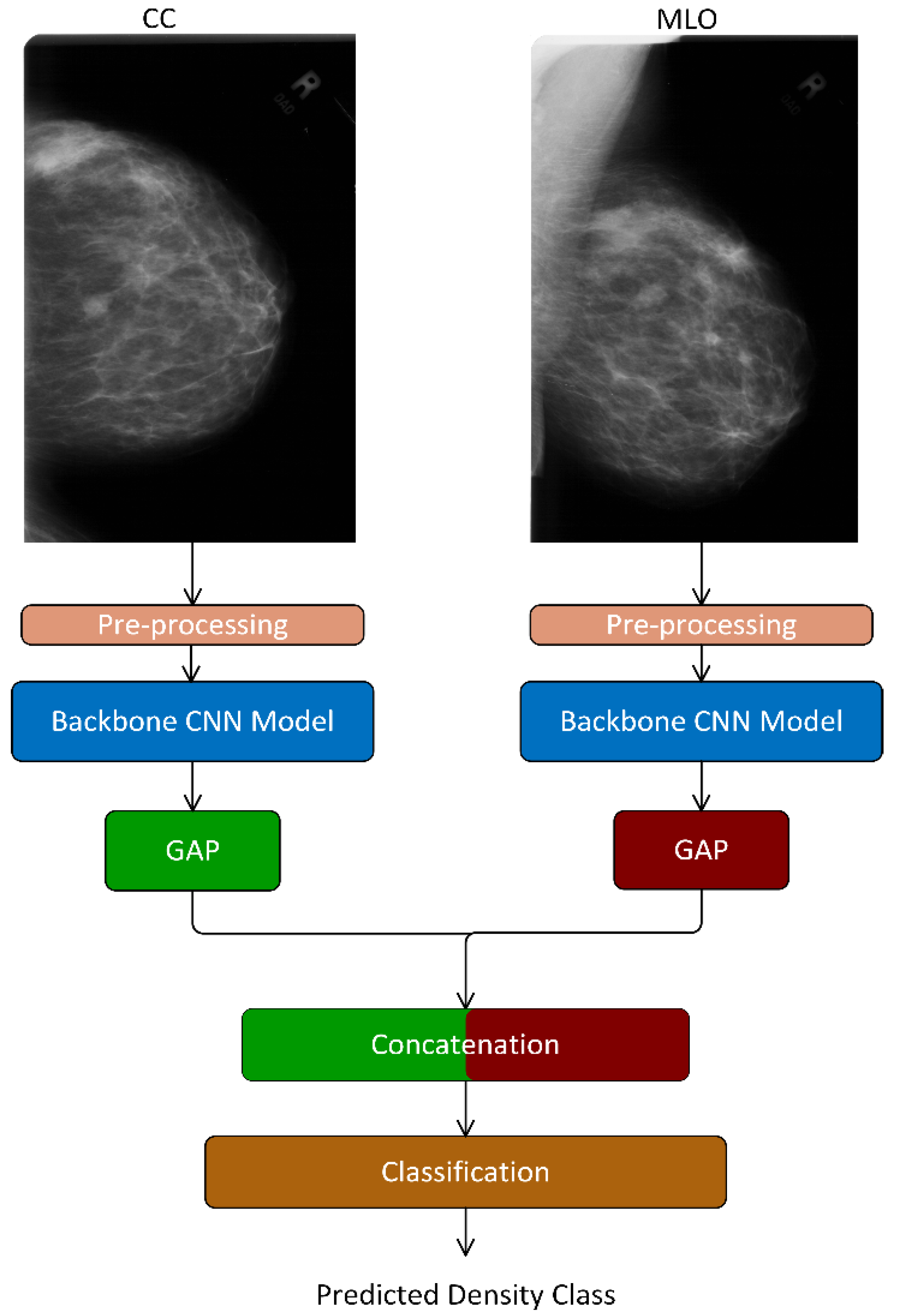
  • We proposed an end-to-end deep learning-based model—TwoViewDensityNet—for the classification of breast density using dual mammogram views, i.e., craniocaudal (CC) view and mediolateral oblique (MLO) view. It combines the CC and MLO views by leveraging the relationship between views and using a CNN as the backbone model. First, it extracts the complementary information from each view using a CNN model, fuses them using a concatenation layer, and finally, predicts the density class using an FC layer with SoftMax activation.
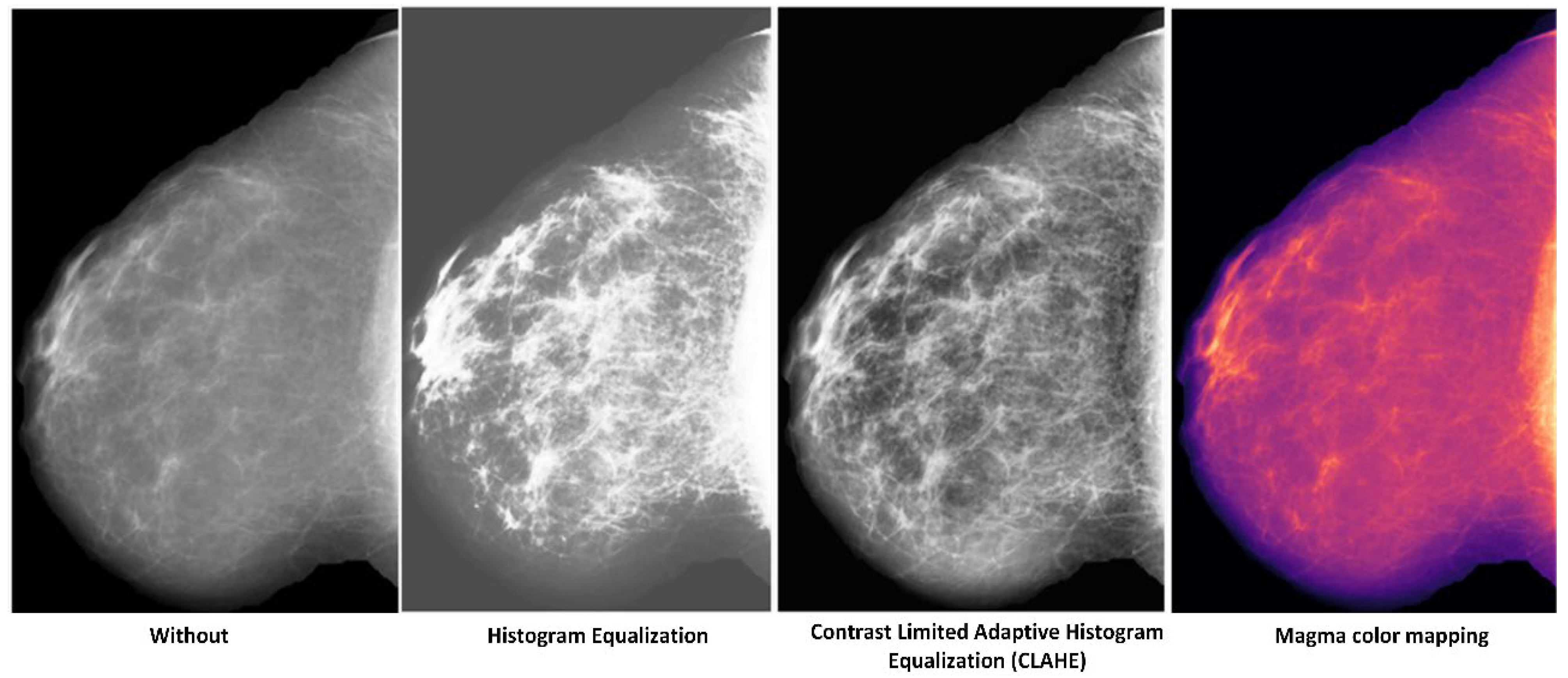
  • We evaluated different preprocessing techniques to enhance the mammogram image before feeding it to the CNN model and found the one that is best suited for the proposed model.
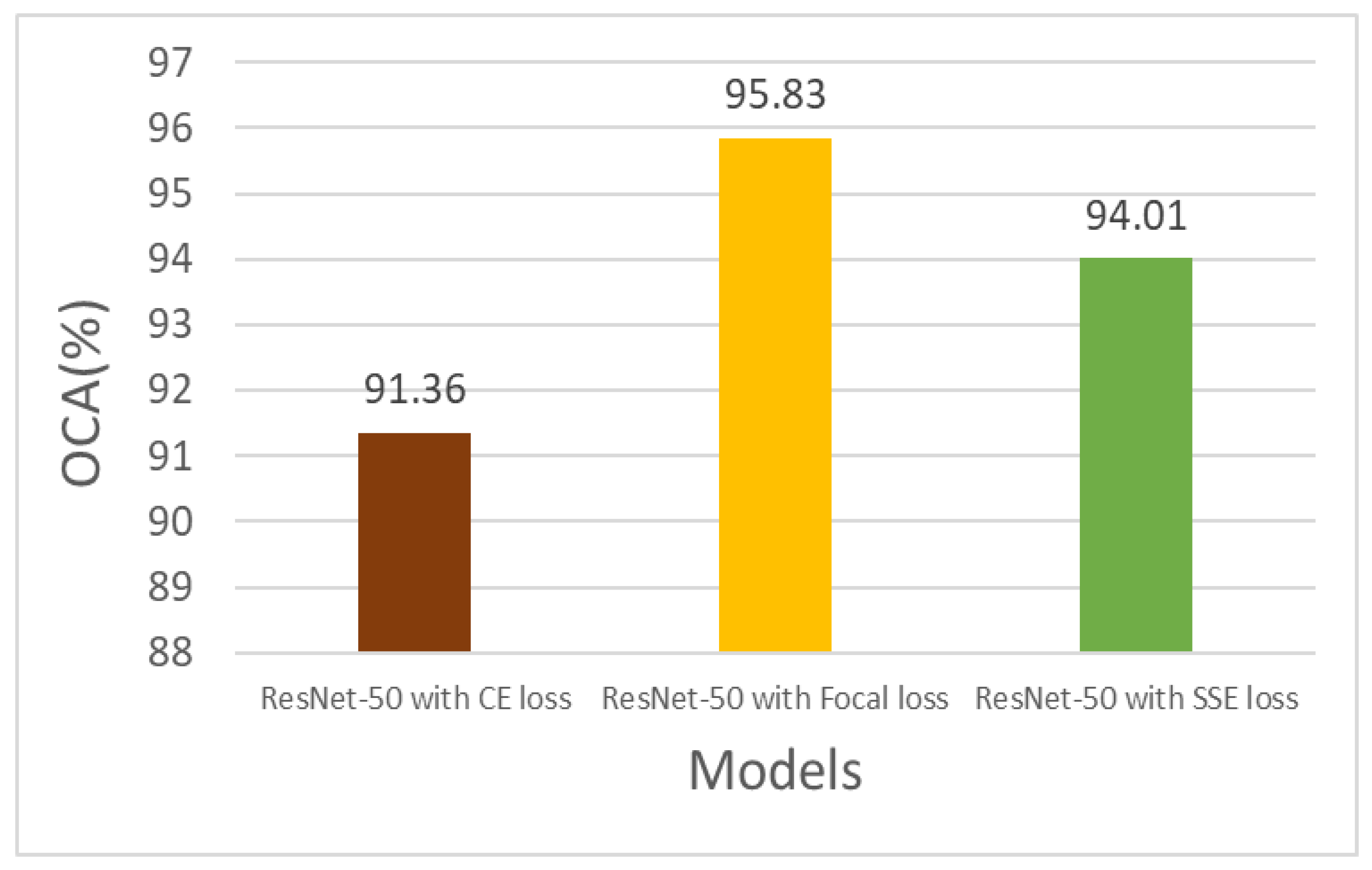
  • We employed different loss functions and their valuable characteristics to tackle the class-imbalance problem.
The remainder of this paper is organized as follows. Section 2 presents previous works related to breast density classification. Section 3 describes the proposed system of four BI-RADS categorizations. We present evaluation protocols in Section 4. Experimental results, as well as their interpretation and discussion, are presented in Section 5. Finally, we end up with the conclusions in Section 6.

2. Related Work

Many researchers have focused their attention on the challenge of classifying breast density into BI-RADS classifications. These approaches were tested with benchmark datasets such as the Digital Database for Screening Mammography (DDSM), INbreast, and Private datasets. Several methods that use deep learning have been proposed, including single-view-based and multi-view-based, reviewed in the following sections. A summary of these studies in the recent literature is presented in Table 1.
Li et al. [7] developed a CNN model based on dilated and attention-guided residual learning for the mammography density classification task. In addition, a multi-stream architecture was designed specifically to analyze multi-view mammograms. They achieved an accuracy of 88.7% and 70.0%, respectively. Yi et al. [8] developed deep convolutional neural networks (DCNNs) based on ResNet-50 to categorize two-dimensional mammography images, determine breast laterality, and assess breast tissue density. Their approach achieved 68% accuracy with breast density classification. Wu et al. [9] proposed a multi-view three-layer CNN to categorize breast density into the four density categories or superclasses (dense and non-dense), using all four mammography views as input. It gave an accuracy of 82.5% for superclasses and a macAUC (macro average) of 0.934 (Class 0: 0.971, Class 1: 0.859, C2: 0.905, and Class 3: 1) for the four-density classification. Lehman et al. [10] proposed deep learning based on ResNet-18 for dense and non-dense and BI-RADS density classification. They showed good agreement (kappa value = 77%) for four BI-RADS categorizations with radiologists in the test set. Zhao et al. [12] proposed a bilateral-view adaptive spatial and channel attention network (BASCNet) based on ResNet-50 as a backbone for fully automated breast density classification by integrating left and right breast information and adaptively capturing distinguishing features in space and channel dimensions. The method achieved accuracies of 85.10% and 90.51%. Gandomkar et al. [13] addressed the fine-tuning of the Inception-V3 model for the classification of breast density (i) fatty or dense, (ii) BI-RADS I, BI-RADS/II, and (iii) BI-RADS III/BI-RADS IV. The method achieved an accuracy of 83.33% and a Cohen’s kappa of 0.775 for four BI-RADS categorizations. Jian et al. [14] developed an attention strategy in which the SE-Attention mechanism is combined with the CNN framework to classify four BI-RADS. This method achieved accuracies of 92.17%, 89.97%, 89.64%, and 89.20% for Inception-V4-SE- Attention, Inception-V4, ResNeXt, and DenseNet models, respectively. Mohamed et al. [15] designed an end-to-end CNN model using improved AlexNet to classify breast density into BI-RADS categories. II and BI-RADS.III. The method achieved an AUC of 0.9421.
The preceding review of state-of-the-art approaches demonstrates that breast density classification requires additional research. All the methods discussed above use the cross-entropy function, which is often used for classification problems. We used different loss functions, such as focal and sum square error loss, to boost the CNN model’s classification accuracy. Additionally, by utilizing different preprocessing approaches to improve the training data provided to the CNN, it is possible to learn various density features. The preceding review of state-of-the-art approaches demonstrates that breast density classification requires additional research. Unilateral mammography images may not contain enough information to accurately classify breast density [7,9,12]. The classification accuracy will be improved by incorporating image information from contralateral or multi-view mammography. Previous studies have based their criteria on multi-view (i.e., four views including left MLO, right MLO, left CC, right CC) or two-view (i.e., similar for two MLO-view or two CC-view). In addition, the training data provided to the CNN requirement of previous studies were based on input images of size 224 × 224, whereas we used input images of size 336 × 224 to accommodate the regular aspect ratio of mammograms.
Timothy and Lakshman [16] developed DualViewNet for density classification similar to our method. The proposed model classifies MLO and CC mammograms taken from the same breast. It gave an AUC of 89.70%. The main difference between this method and our approach is the architecture of the deep models. The method in [16] extracts features using convolutional layers of two deep models, concatenates them, and classifies them; As the features from the convolutional layers are concatenated directly, so the dimension of the feature space becomes very high, which leads to classification layer with a huge number of learnable parameters. It restricts the use of only the CNN models with a reduced number of parameters, such as MobileNetV2, to avoid overfitting. On the contrary, our method first extracts features using the convolutional layers of deep models, then reduces the dimension of the feature space using global average pooling (GAP) layers and concatenates them. In this way, the dimension of the feature space is significantly reduced, and the parameter complexity of the classification layer remains very low. It allows using any pretrained CNN model as a backbone avoiding the fear of overfitting. Moreover, we first extract the breast area, unlike the method in [16], to emphasize the breast density, not just color mapping to magma and resizing to 336 × 224.

3. Proposed Method

In mammography, two views, i.e., CC and MLO, of the ipsilateral breast (i.e., two-view analysis) and the corresponding views of the contralateral breast (i.e., bilateral analysis) are captured to analyze the breast for detecting possible abnormalities. Both views have a complementary relationship and reveal signs of an abnormality better than a single view. Various multi-view approaches were proposed to improve the detection of breast abnormalities in mammograms. Multiple views of the right and left breasts in CC and MLO views are used to derive the information for these procedures. The ipsilateral analysis is based on combining the different projection views of the same breast, and bilateral analysis is based on combining the same projection view of the left and right breast [17,18,19,20,21]. This observation has been employed in different techniques for mass classification [22,23,24] and density classification. These studies reveal that multi-views result in better performance than a single view. Inspired by this, we propose a prediction model for breast density classification into four BI-RADS categories based on dual views, as shown in Figure 2. The proposed technique is an end-to-end deep learning-based model (we call it TwoViewDensityNet) that takes two views, i.e., two mammogram images of size 336 × 224 as input and predicts the label of the density type of the breast according to BI-RADS classification. It consists of two branches, one for each view. First, each branch preprocesses the corresponding view and extracts hierarchical features using a convolutional neural network (CNN) as a backbone model. The features from the two views are fused by the concatenation layer and passed to an FC layer, which serves as a classifier and yields the prediction label of the input mammographic views.
The precise specification of this method relies on three important design decisions: (i) which preprocessing technique is suitable, (ii) which backbone CNN model is suited for this task, and (iii) which loss function helps to train the model so that it has good generalization. Each of these design decisions is discussed in detail in the following subsections.

3.1. Preprocessing

Breast tissue is crucial for discrimination between different breast density classes; it must be adequately separated from the background. Removing all artifacts from the image leaves only the breast tissue area for the model to learn from. In the first step, we used the threshold value 200 to generate a binary mask, where 0 (black) is the background pixel, and 1 (white) is the breast region, artifact, or noise pixel. Afterward, a morphological opening operator is applied to the binary image with a disk-type structuring element of size 9 × 9 to extract the breast tissue area; it is more prominent than any object; it is binarized as a single region. As a result, the most significant contours are retained, and the remainder is discarded. Then, we overlay this mask to eliminate mammography artifacts and keep only the breast tissue area. Then, the bounding box of the breast tissue is used to crop each view so that it mainly contains the breast tissue.
Furthermore, we use magma color mapping from 16-bit grayscale to 24-bit RGB, as used in [16]; it enhances the perceptual quality [25,26] of the fibroglandular tissue and fat tissue. In addition, it maps the gray-level mammogram image on an RGB image, which can be passed easily to pretrained CNN models, which are usually pretrained on RGB pictures from ImageNet [27]. Figure 3 illustrates the whole preprocessing process.

3.2. Backbone Convolutional Neural Network (CNN) Model

The TwoViewDensityNet model employs two convolutional neural networks for feature extraction from each view. Greater depth in CNN models allows for extracting discriminative features, improving classification performance. Various widely used deep convolutional models, such as ResNet50 [28], EfficientNetb0 [29], and DenseNet201 [30], etc., can be exploited for feature extraction. We used ResNet-50 pretrained on ImageNet [27]; its architecture is based on residual learning, which allows increasing the depth of a CNN model that prevents the problem of gradient vanishing [31] and degradation [32,33].

3.3. Concatenation Layer

Different techniques combine the extracted deep features from the two views, such as concatenation and element-wise operations. In our proposed method, the features from the two views are fused by the concatenation layer. The output of the global average pooling (GAP) of ResNet-50 in the left branch is x 1 = [ α 1 ,   α 2 , , α 2048 ] T , and the right branch is x 2 = [ β 1 ,   β 2 , , β 2048 ] T . To fuse features from both views, we concatenate them in x where x = [ α 1 ,   α 2 , , α 2048 , β 1 ,   β 2 , , β 2048 ] .

3.4. Classification Layer

The last layer of the model is the classification layer; it is a fully connected layer with four output neurons to classify the input views into one of the four breast density categories; each neuron represents a different BI-RADS class. The output FC layer employs a SoftMax function as an activation function because it is the most commonly used activation function in the output layer; it converts the numerical output of a convolutional neural network to class-specific probability values. The predicted class of the input views is the one for which the posterior probability is maximum. The difference between the predicted class and the actual label is then calculated using a loss function at each training iteration.

3.5. Training the TwoViewDensityNet

The training of the network is an iterative process, and it depends on how accurately the error made by the network is measured, i.e., how the loss function is defined. First, we discuss the loss functions and then describe the optimization method used for training.

3.5.1. Loss Functions

The critical component of a deep-learning algorithm is the loss function; it indicates how much error a neural network makes in recognizing the input image. A sample’s involvement in the optimization problem is measured using a loss function, which assigns a numerical value to each input instance, i.e., the loss. The model parameters are updated so that the loss is minimum. We adopt some well-known loss functions.
Weighted cross-entropy loss (WCE) [34].
Let K be the number of classes and N the number of training instances in a batch. Further, let y n i   be the predicted posterior probability of n t h training example in the batch that belongs to i t h class, then the weighted cross-entropy loss function is calculated as follows in Equation (1):
L o s s = 1 N n = 1 N i = 1 K w i T n i ln y n i
where T n i   is the true posterior probability of n t h training example in the batch that belongs to an i t h class (in one-hot encoding vector), and w i is the prior of the i t h class. Further, if the total batch size is N and the number of instances of the i t h class is m i , then w i = m i N .
Focal loss (FL) [35].
Let K be the number of classes and N the number of training instances in a batch. Further, let y n i   be the predicted posterior probability of n t h training example in the batch that it belongs to i t h class, then the focal loss function is calculated as follows in Equation (2):
L o s s = 1 N n = 1 N i = 1 K T n i α ( 1 y n i ) γ ln y n i
where T n i   is the true posterior probability of n t h training example in the batch that belongs to an i t h class, and γ is the focusing parameter where γ ϵ [ 0 , 0.5 ] .
Sum square error loss (SSE) [36].
Let K be the number of classes and N the number of training instances in a batch. Further, let y n i   be the predicted posterior probability of the n t h training example in the batch that belongs to the i t h class, then the sum square error loss function is calculated as follows in Equation (3):
L o s s = 1 N n = 1 N i = 1 K ( y n i T n i ) 2
where T n i   is the true posterior probability of n t h training example in the batch that belongs to an i t h class.

3.5.2. Algorithms Used for Training
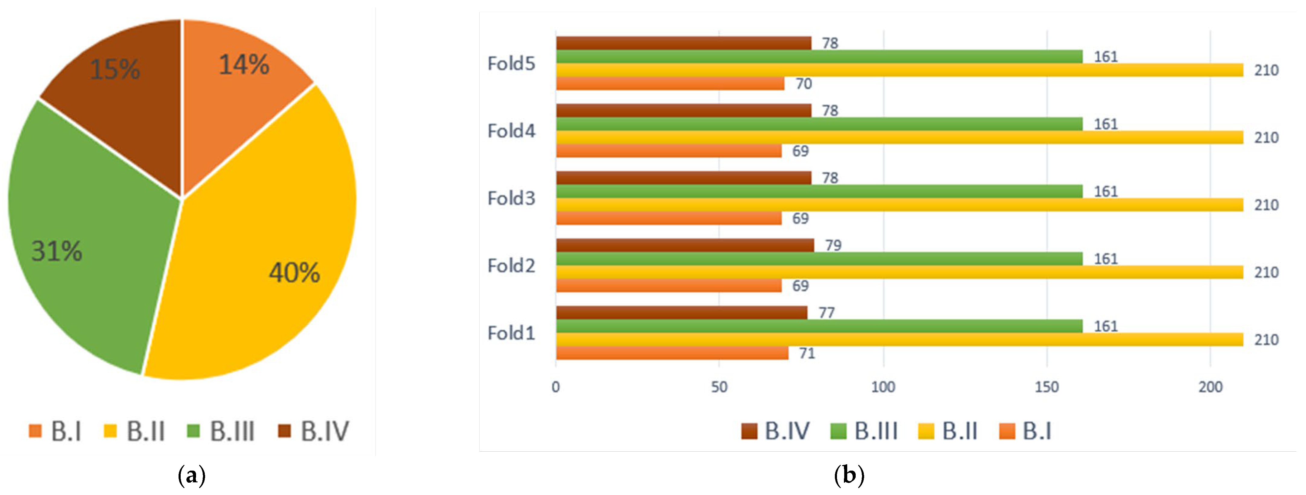
Fine-tuning involves various hyper-parameters: the optimization algorithm, learning rate, batch size, and the number of training epochs. We attempt different options to determine the best values of the hyperparameters. We tested three optimizers (Adam, SGD, and RMSprop), a learning rate between 1 × 10⁻⁴ and 1 × 10⁻², four batch sizes (16, 32, 64), and the number of epochs between 50 and 100. Early stopping is performed with patience of seven iterations to further reduce overfitting. Finally, we have decided on stochastic gradient descent (SGD) optimizers to fine-tune the models with a momentum of 0.9 and an initial learning rate of 1 × 10 4 . The training epoch is 50, and the batch size is 64; this would result in approximately 3–4 h of runtime.

3.5.3. Datasets

To verify the proposed system’s efficiency and robustness, we employed two publicly available mammographic benchmark datasets:
Digital Database for Screening Mammography (DDSM) [11]. The DDSM database consists of 2620 mammography screening cases containing a total of 10,480 mammograms with a resolution of 4000 × 6000 pixels. Moreover, they are stored in portable gray map (PGM) format with 16 bits; every case includes two views of bilateral breasts craniocaudal (CC), mediolateral oblique (MLO), breast laterality (right vs. left), and Breast Imaging Reporting and Data System (BI-RADS) breast density (four categories: almost entirely fatty, scattered area of fibroglandular density, heterogeneously dense, and extremely dense). We selected two views of each breast density category, totaling 5406 images, and the image distribution over the four categories presented in Figure 4a. Five-fold cross-validation is used to train and test models. Figure 4b shows the data distribution for each fold.
INbreast [37] is taken from the Breast Centre at the University of Hospital de São João, Portugal. It contains 115 cases comprising digital images converted to DICOM format with a resolution of either 3328 × 4084 or 2560 × 3328 pixels. Each case includes both craniocaudal (CC) and mediolateral oblique (MLO) views and breast laterality (right vs. left) annotated with contour points of the ROIs. The density labels are annotated by radiologists as BI-RADS I, BI-RADS II, BI-RADS III, and BI-RADS IV. Out of the total number of BI-RADS categories, 136 belong to BI-RADS I, 147 to BI-RADS II, 99 to BI-RADS III, and 28 to BI-RADS IV. Furthermore, 5-fold cross-validation is used to train and test models.

3.5.4. Data Augmentation

Training a CNN model on a large number of training instances typically yields good results and high-performance values. Additionally, data imbalances may be alleviated with the use of augmentation techniques. To reproduce a large number of breast density variations in mammogram images, we used rotation (θ = 180°) and random horizontal and vertical flipping.

4. Evaluation Protocol

We randomly divided the data into a training set (80%), a validation set (10%), and a test set (10%) and used a 5-fold cross-validation technique to evaluate the proposed system. The cross-validation concept is based on partitioning the dataset into k equal-sized folds. Then, k 1 folds will be used to train and validate, with the remaining fold to test the classification models. The final result is calculated as the average of overall classes [38].
Using the confusion matrix in Table 2, a model’s classification performance is evaluated primarily in terms of overall class accuracy (OCA), individual class accuracy (ICA), recall (RC), precision (PR), F1-score, Cohen’s kappa [39,40,41]. The definitions of these performance measures are described with the help of Equations (4)–(8), as shown below:
Overall   Classification   Accuracy   ( OCA . ) = Correct   predictions Total   predictions  
Individual   Classification   Accuracy   ( ICA . ) = Correct   predictions   belong   to   a   specific   class Total   predictions   belong   to   a   specific   class
Precision = Tp TP + FP   Recall = Tp TP + FN
F 1   Score = 2 × Precision × Recall   Precision + Recall
Cohen’s kappa is calculated using the following:
Kappa = ( P o P e ) ( 1 P e )   P e = ( T P + F N ) × ( T P + F P ) + ( F P + T N ) × ( F N + T N ) ( T P + T N + F P + F N ) 2 ;   P o = T P + T N T P + T N + F P + F N
Additionally, the breast density classifier’s performance was measured using the area under the ROC curve (AUC). The area under the receiver operating characteristic (AUC-ROC) curve is used to evaluate the effectiveness of classification problems with varying thresholds [42,43]. AUC is the separability measure, while ROC is a probability curve. It reveals the extent to which the model can differentiate between different types of data. The multiclass classifier considers the AUC between each class and all other classes (a one vs. all approach).
The system was implemented, and all experiments were performed in MATLAB R2021b version 9.11 with a deep-learning toolbox on AMD Ryzen Threadripper 3960X 24-core processor, 3.79 GHz, RAM 128 GB, and Nvidia graphics processing units (GPU) based in Santa Clara, CA, USA, GeForce RTX 3090 24 GB.

5. Experimental Results and Discussion

5.1. Ablation Study

This section conducts different ablation tests to validate the proposed system structure’s efficiency.

5.1.1. Which Backbone Model?

The question of which CNN model to use as the system’s backbone is emerging. The DDSM dataset was used to test three state-of-the-art CNN models. Based on the obtained results illustrated in Table 3, the selected backbone model for the breast density classification task was the ResNet-50. This decision was made because ResNet-50 outperformed other models in terms of overall classification accuracy. The variation in performance amongst the investigated CNN models can be attributable to the different design choices.

5.1.2. Which Preprocessing Operation?

Breast tissue characteristics in digital mammographic images will be more apparent after image enhancement, increasing the early breast cancer classification rate. A custom-tailored image processing technique will likely be needed to best display different image characteristics. Additionally, different breast density may benefit from specific algorithms and the performance disparities between the image preprocessing methods. As a result, we decided on magma color mapping, as presented in Table 4. An overview of different image preprocessing tasks is shown in Figure 5.

5.1.3. Single View or Dual View?

Comparing the results utilizing dual-view mammography inputs to those using single-view mammography input, it can be observed that the dual-view mammography inputs setting is beneficial to the density classification task, and improved statistics were obtained by all of the investigated models, including the backbone model ResNet50, as shown in Table 5.

5.1.4. Which Loss Function?

As mentioned in Section 3.5.1, We considered three loss functions: cross-entropy, focal, and SSE. We used the pretrained ResNet50 model as the backbone CNN model to test the effect of these loss functions. Figure 6 and Figure 7 show the results of the three-loss function on the DDSM dataset. The focal loss function yields the best results in terms of all performance metrics because focal loss does this by decreasing the weight given to simple examples in the loss function, hence focusing on more hard examples. Table 6 shows the results. In Table 7, we provide the confusion matrix produced from the best experiment result to explore the classification behavior of the model.

5.2. Comparison with State-of-the-Art Methods for Breast Density Classification

The method of Zhao et al. [12] has been introduced to compare related methods of the DDSM dataset with a four-view. The bilateral adaptive spatial and channel attention network (BASCNet) integrates the information of the left and right breasts. Li et al. [7] added dilated convolution and the channel attention mechanism to the ResNet network architecture with multi-view inputs (i.e., four-view, as well as two CC views or two MLO views of the left and right breasts). Wu et al. [9] used a VGG Net with four views as input. Our proposed method TwoViewDensityNet significantly outperforms the state-of-the-art methods since we used two views, CC and MLO, from the same breast.
Additionally, we applied different loss functions to improve performance accuracy. Our proposed method attained the highest accuracy of 95.83 on the DDSM, respectively, when TwoViewDensityNet used ResNet-50 as the backbone model with focal loss function; this is significantly higher than the existing methods. The findings were compared using a dual-view input. With a single-view input, it is evident that the dual-view input option is beneficial to the classification task and the ResNet50 backbone produced those improved metrics. Compared to Zhao et al. [12] on DDSM, our proposal outperformed w.r.t. all evaluation metrics, as presented in Table 8. To be precise, our model increased classification accuracy by 10% and 5% F1 score by 20% and 19% on the DDSM and INbreast, respectively, for dual-view inputs.

5.3. Discussion

Utilizing the dual-view approach, we built and tested a system for classifying breast density tissue as B-I, B-II, B-III, or B-IV using the DDSM benchmark dataset as guidance. An end-to-end CNN model was utilized as the backbone model in the method. We combined the information from two views and learned which complementary information is essential in each view. When we fine-tune this backbone for left and right, each view’s weight and complementary information are classified. Among the well-known CNN models, we investigated (ResNet-50, DenseNet-201, and Efficient-b0) and determined that ResNet-50 is the most suitable model for the system. That might be residual learning extracting global (high-level) features that effectively pay more attention to the semantics of fibroglandular tissue, which enables accurate discrimination of the four BI-RADS categories.
This study has some limitations. However, for the mammography dataset used in this study, the accessible images were limited, resulting in a severely uneven distribution across the four categories. Training a classification network with these datasets is quite difficult. Furthermore, breast density is a critical clinical characteristic used to determine a woman’s risk of developing breast cancer. Our proposed system is well classified between non-dense breasts (fatty or scattered density) and dense breasts (heterogeneously dense or extremely dense). It is simple to differentiate between fatty and highly dense breasts in the clinical setting.
On the other hand, radiologists have difficulty visually and consistently distinguishing between the scatter density and heterogeneously dense categories [44]. According to our findings, the heterogeneously dense or extremely dense classification results are better than the fatty or scattered density; this might be because of the similar characteristic between fatty and heterogeneously dense or scattered density and extremely dense.
The performance of TwoViewDensityNet for the four BI-RADS classification tasks on the DDSM dataset is (F-score of 98.63%, AUC of 99.51%, accuracy of 95.83%) and the INbreast dataset is (F-score of 97.14%, AUC of 97.44%, accuracy of 96%).

6. Conclusions

We addressed the challenging problem of discriminating mammographic breast density and, by leveraging advances in deep learning, developed a system for this problem that leverages the complementary relationship between the craniocaudal (CC) and mediolateral oblique (MLO) views to improve the differentiation of BI-RADS class. We extensively tested the system on the benchmark datasets DDSM and INbreast and discovered that it outperforms the state-of-the-art approaches. ResNet-50 achieves better results as a backbone model for the system when focal loss is used for training. We will continue investigating deep-learning mammography models and develop more robust models. This would help radiologists enhance the current clinical breast density assessment. The proposed model can be used for other similar applications, which will be our future work.

Author Contributions

Conceptualization, M.B. and M.H.; Data curation, M.B. and S.A.A.S.; Formal analysis, M.B. and S.A.A.S.; Funding acquisition; Methodology, M.B., F.-e.-A. and M.H.; Project administration, F.-e.-A. and M.H.; Resources, F.-e.-A. and M.H.; Software, M.B.; Supervision, M.H. and H.A.A.; Validation, M.B.; Visualization, M.B.; Writing—original draft preparation, M.B.; Writing—review and editing, M.H. All authors have read and agreed to the published version of the manuscript.

Funding

The authors extend their appreciation to the Deputyship for Research & Innovation, Ministry of Education in Saudi Arabia for funding this research work through the project no. (IFKSURG-2-106).

Data Availability Statement

The DDSM dataset is available at: http://www.eng.usf.edu/cvprg/Mammography/Database.html (accessed on 25 November 2021).

Conflicts of Interest

The authors declare no conflict of interest.

References

  1. Wolfe, J.N. Risk for breast cancer development determined by mammographic parenchymal pattern. Cancer 1976, 37, 2486–2492. [Google Scholar] [CrossRef] [PubMed]
  2. Wolfe, J.N. Breast patterns as an index of risk for developing breast cancer. Am. J. Roentgenol. 1976, 126, 1130–1137. [Google Scholar] [CrossRef] [PubMed]
  3. McCormack, V.A.; dos Santos Silva, I. Breast Density and Parenchymal Patterns as Markers of Breast Cancer Risk: A Meta-analysis. Cancer Epidemiol. Biomark. Prev. 2006, 15, 1159–1169. [Google Scholar] [CrossRef] [PubMed] [Green Version]
  4. Nazari, S.S.; Mukherjee, P. An overview of mammographic density and its association with breast cancer. Breast Cancer 2018, 25, 259–267. [Google Scholar] [CrossRef] [PubMed] [Green Version]
  5. Albeshan, S.M.; Hossain, S.Z.; Mackey, M.G.; Peat, J.K.; Al Tahan, F.M.; Brennan, P.C. Preliminary investigation of mammographic density among women in Riyadh: Association with breast cancer risk factors and implications for screening practices. Clin. Imaging 2019, 54, 138–147. [Google Scholar] [CrossRef]
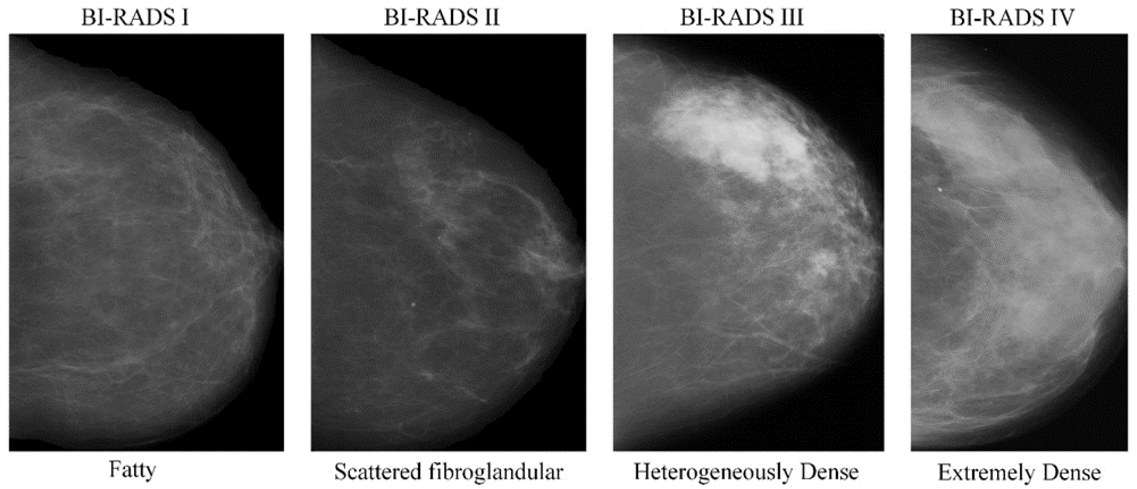
  6. American College of Radiology (ACR). Illustrated Breast Imaging Reporting and Data System (BI-RADS); American College of Radiology: Reston, VA, USA, 2003. [Google Scholar]
  7. Li, C.; Xu, J.; Liu, Q.; Zhou, Y.; Mou, L.; Pu, Z.; Xia, Y.; Zheng, H.; Wang, S. Multi-View Mammographic Density Classification by Dilated and Attention-Guided Residual Learning. IEEE/ACM Trans. Comput. Biol. Bioinform. 2020, 18, 1003–1013. [Google Scholar] [CrossRef]
  8. Yi, P.H.; Lin, A.; Wei, J.; Yu, A.C.; Sair, H.I.; Hui, F.K.; Hager, G.D.; Harvey, S.C. Deep-Learning-Based Semantic Labeling for 2D Mammography and Comparison of Complexity for Machine Learning Tasks. J. Digit. Imaging 2019, 32, 565–570. [Google Scholar] [CrossRef] [Green Version]
  9. Wu, N.; Geras, K.J.; Shen, Y.; Su, J.; Kim, S.G.; Kim, E.; Wolfson, S.; Moy, L.; Cho, K. Breast Density Classification with Deep Convolutional Neural Networks. In Proceedings of the 2018 IEEE International Conference on Acoustics, Speech and Signal Processing (ICASSP), Calgary, AB, Canada, 15–20 April 2018; pp. 6682–6686. [Google Scholar]
  10. Lehman, C.D.; Yala, A.; Schuster, T.; Dontchos, B.; Bahl, M.; Swanson, K.; Barzilay, R. Mammographic Breast Density Assessment Using Deep Learning: Clinical Implementation. Radiology 2019, 290, 52–58. [Google Scholar] [CrossRef] [Green Version]
  11. Heath, M.; Bowyer, K.; Kopans, D.; Kegelmeyer, P.; Moore, R.; Chang, K.; Munishkumaran, S. Current Status of the Digital Database for Screening Mammography. In Digital Mammography; Springer: Dordrecht, The Netherlands, 1998. [Google Scholar]
  12. Zhao, W.; Wang, R.; Qi, Y.; Lou, M.; Wang, Y.; Yang, Y.; Deng, X.; Ma, Y. BASCNet: Bilateral adaptive spatial and channel attention network for breast density classification in the mammogram. Biomed. Signal Process. Control. 2021, 70, 103073. [Google Scholar] [CrossRef]
  13. Gandomkar, Z.; Suleiman, M.E.; Demchig, D.; Brennan, P.C.; McEntee, M.F. BI-RADS Density Categorization Using Deep Neural Networks. In Medical Imaging 2019: Image Perception, Observer Performance, and Technology Assessment; SPIE: Bellingham, WA, USA, 2019. [Google Scholar]
  14. Deng, J.; Ma, Y.; Li, D.A.; Zhao, J.; Liu, Y.; Zhang, H. Classification of breast density categories based on SE-Attention neural networks. Comput. Methods Programs Biomed. 2020, 193, 105489. [Google Scholar] [CrossRef]
  15. Mohamed, A.A.; Berg, W.A.; Peng, H.; Luo, Y.; Jankowitz, R.C.; Wu, S. A deep learning method for classifying mammographic breast density categories. Med. Phys. 2017, 45, 314–321. [Google Scholar] [CrossRef] [PubMed]
  16. Cogan, T.; Tamil, L.S. Deep Understanding of Breast Density Classification. In Proceedings of the 42nd Annual International Conference of the IEEE Engineering in Medicine & Biology Society (EMBC), Montreal, QC, Canada, 20–24 July 2020; pp. 1140–1143. [Google Scholar]
  17. Jouirou, A.; Baâzaoui, A.; Barhoumi, W. Multi-view information fusion in mammograms: A comprehensive overview. Inf. Fusion 2019, 52, 308–321. [Google Scholar] [CrossRef]
  18. Wilms, M.; Krüger, J.; Marx, M.; Ehrhardt, J.; Bischof, A.; Handels, H. Estimation of Corresponding Locations in Ipsilateral Mammograms: A Comparison of Different Methods. In Medical Imaging 2015: Computer-Aided Diagnosis; SPIE: Bellingham, WA, USA, 2015. [Google Scholar]
  19. Ma, Y.; Peng, Y. Simultaneous detection and diagnosis of mammogram mass using bilateral analysis and soft label based metric learning. Biocybern. Biomed. Eng. 2022, 42, 215–232. [Google Scholar] [CrossRef]
  20. Xian, J.; Wang, Z.; Cheng, K.-T.; Yang, X. Towards Robust Dual-View Transformation via Densifying Sparse Supervision for Mammography Lesion Matching. In Proceedings of the International Conference on Medical Image Computing and Computer-Assisted Intervention, Strasbourg, France, 27 September 2021. [Google Scholar]
  21. Kowsalya, S.; Priyaa, D.S. An Adaptive Behavioral Learning Technique based Bilateral Asymmetry Detection in Mammogram Images. Indian J. Sci. Technol. 2016, 9, S1. [Google Scholar] [CrossRef]
  22. Lyu, Q.; Namjoshi, S.V.; McTyre, E.; Topaloglu, U.; Barcus, R.; Chan, M.D.; Cramer, C.K.; Debinski, W.; Gurcan, M.N.; Lesser, G.J.; et al. A transformer-based deep learning approach for classifying brain metastases into primary organ sites using clinical whole brain MRI images. Patterns 2022, 3, 100613. [Google Scholar] [CrossRef]
  23. Dhungel, N.; Carneiro, G.; Bradley, A.P. Fully Automated Classification of Mammograms Using Deep Residual Neural Networks. In Proceedings of the IEEE 14th International Symposium on Biomedical Imaging (ISBI 2017), Melbourne, Australia, 18–21 April 2017; pp. 310–314. [Google Scholar]
  24. Yi, D.; Sawyer, R.L.; Cohn, D.; Dunnmon, J.A.; Lam, C.K.; Xiao, X.; Rubin, D. Optimizing and Visualizing Deep Learning for Benign/Malignant Classification in Breast Tumors. arXiv 2017, arXiv:1705.06362. [Google Scholar]
  25. Cogan, T.; Cogan, M.; Tamil, L.S. RAMS: Remote and automatic mammogram screening. Comput. Biol. Med. 2019, 107, 18–29. [Google Scholar] [CrossRef]
  26. MatPlotLib Perceptually Uniform Colormaps. Available online: https://www.mathworks.com/matlabcentral/fileexchange/62729-matplotlibperceptually-uniform-colormaps (accessed on 25 November 2021).
  27. Russakovsky, O.; Deng, J.; Su, H.; Krause, J.; Satheesh, S.; Ma, S.; Huang, Z.; Karpathy, A.; Khosla, A.; Bernstein, M.; et al. ImageNet Large Scale Visual Recognition Challenge. Int. J. Comput. Vis. 2015, 115, 211–252. [Google Scholar] [CrossRef] [Green Version]
  28. KHe, K.; Zhang, X.; Ren, S.; Sun, J. Deep Residual Learning for Image Recognition. In Proceedings of the 2016 IEEE Conference on Computer Vision and Pattern Recognition (CVPR), Las Vegas, NV, USA, 27–30 June 2016; pp. 770–778. [Google Scholar] [CrossRef] [Green Version]
  29. Tan, M.; Le, Q.V. EfficientNet: Rethinking Model Scaling for Convolutional Neural Networks. In Proceedings of the International Conference on Machine Learning, Long Beach, CA, USA, 10–15 June 2019. [Google Scholar]
  30. Huang, G.; Liu, Z.; Van Der Maaten, L.; Weinberger, K.Q. Densely Connected Convolutional Networks. In Proceedings of the 2017 IEEE Conference on Computer Vision and Pattern Recognition (CVPR), Honolulu, HI, USA, 21–26 July 2017; pp. 2261–2269. [Google Scholar]
  31. Veit, A.; Wilber, M.J.; Belongie, S. Residual Networks Behave Like Ensembles of Relatively Shallow Networks. In Proceedings of the Advances in Neural Information Processing Systems 29, Barcelona, Spain, 5–10 December 2016; pp. 550–558. [Google Scholar]
  32. Schmidhuber, J. Deep Learning in Neural Networks: An Overview. Neural Netw. 2015, 61, 85–117. [Google Scholar] [CrossRef] [Green Version]
  33. Glorot, X.; Bengio, Y. Understanding the Difficulty of Training Deep Feedforward Neural Networks. In Proceedings of the 13th International Conference on Artificial Intelligence and Statistics (AISTATS), Sardinia, Italy, 13–15 May 2010; pp. 249–256. [Google Scholar]
  34. De Boer, P.T.; Kroese, D.P.; Mannor, S.; Rubinstein, R.Y. A Tutorial on the Cross-Entropy Method. Ann. Oper. Res. 2005, 134, 19–67. [Google Scholar] [CrossRef]
  35. Lin, T.Y.; Goyal, P.; Girshick, R.; He, K.; Dollár, P. Focal Loss for Dense Object Detection. In Proceedings of the IEEE Transactions on Pattern Analysis and Machine Intelligence, Venice, Italy, 22–29 October 2017. [Google Scholar]
  36. Bosman, A.S.; Engelbrecht, A.; Helbig, M. Visualising basins of attraction for the cross-entropy and the squared error neural network loss functions. Neurocomputing 2020, 400, 113–136. [Google Scholar] [CrossRef] [Green Version]
  37. Moreira, I.C.; Amaral, I.; Domingues, I.; Cardoso, A.; Cardoso, M.J.; Cardoso, J.S. Inbreast: Toward a full-field digital mammographic database. Acad. Radiol. 2012, 19, 236–248. [Google Scholar] [CrossRef] [PubMed] [Green Version]
  38. Levin, E.; Fleisher, M. Accelerated learning in layered neural networks. Complex Syst. 1988, 2, 625–640. [Google Scholar]
  39. Stone, M. Cross-validatory choice and assessment of statistical predictions. J. R. Stat. Soc. 1974, 36, 111–147. [Google Scholar] [CrossRef]
  40. Cetin, K.; Oktay, Y.; Sinan, A. Performance Analysis of Machine Learning Techniques in Intrusion Detection. In Proceedings of the 24th Signal Processing and Communication Application Conference (SIU), Zonguldak, Turkey, 16–19 May 2016; pp. 1473–1476. [Google Scholar]
  41. Ranganathan, P.; Pramesh, C.S.; Aggarwal, R. Common pitfalls in statistical analysis: Measures of agreement. Perspect. Clin. Res. 2017, 8, 187–191. [Google Scholar] [CrossRef]
  42. Hanley, J.A.; McNeil, B.J. The meaning and use of the area under a receiver operating characteristic (ROC) curve. Radiology 1982, 143, 29–36. [Google Scholar] [CrossRef] [Green Version]
  43. Hoo, Z.H.; Candlish, J.; Teare, D. What is an ROC curve? Emerg. Med. J. 2017, 34, 357–359. [Google Scholar] [CrossRef] [Green Version]
  44. Sprague, B.L.; Conant, E.F.; Onega, T.; Garcia, M.P.; Beaber, E.F.; Herschorn, S.D.; Lehman, C.D.; Tosteson, A.N.; Lacson, R.; Schnall, M.D.; et al. Variation in Mammographic Breast Density Assessments Among Radiologists in Clinical Practice: A Multicenter Observational Study. Ann. Intern. Med. 2016, 165, 457–464. [Google Scholar] [CrossRef]
Figure 1. Examples of BI-RADS breast composition categories of breast density in increasing order of density from left to right [11].
Mathematics 10 04610 g001
Figure 2. Proposed density classification system. GAP stands for global average pool.
Mathematics 10 04610 g002
Figure 3. Preprocessing method for mammogram image.
Mathematics 10 04610 g003
Figure 4. (a) Data distribution of the DDSM dataset over the four classes; (b) data distribution of the DDSM dataset for each fold.
Mathematics 10 04610 g004
Figure 5. A comparison of the visual effects of different image preprocessing tasks.
Mathematics 10 04610 g005
Figure 6. The effect of different loss functions of the DDSM test on overall classification accuracy.
Mathematics 10 04610 g006
Figure 7. The effect of different loss functions of the DDSM test individual classification accuracy.
Mathematics 10 04610 g007
Table 1. The comparison with different state-of-the-art methods for breast density classification.
ReferencesModelDatasetACC (%)AUC (%)F1-Score (%)
Single View
Li et al. [7] (2021)ResNet50 + DC + CA
(DC: dilated convolutions. CA:channel-wise attention)
Private88.7097.4087.10
INbreast7084.7063.50
Jian et al. [14] (2020)Inception-V4-SE- AttentionPrivate92.17--
ResNeXt-SE-Attention andPrivate89.97
DenseNet-SE-AttentionPrivate89.64
Yi et al. [8] (2019)ResNet-50DDSM68--
Lehman et al. [10] (2019)ResNet-18Private77--
Gandomkar et al. [13] (2019)Inception-V3Private83.33-77.50
Mohamed et al. [15] (2018)AlexNetPrivate-92-
Multi-View
Zhao et al. [12] (2021)BASCNet (ResNet)
(Bilateral-view adaptive spatial and channel attention network)
DDSM85.1091.5478.92
INbreast90.5199.0978.11
Li et al. [7] (2021)ResNet50 + DC + CA
(DC: dilated convolutions. CA: channel-wise attention)
Private92.1098.191.2
92.5098.291.7
75.2093.667.9
Timothy and Lakshman
[16] (2020)
DualViewNetCBISDDSM-89.70-
Wu et al. [9] (2018)VGG NetPrivate69.4084.20-
Table 2. Confusion matrix.
Confusion MatrixActual PositiveActual Negative
Predicted PositiveTP 1FP 3
Predicted NegativeFN 4TN 2
1 The number of true positives (TPs): the prediction was positive when the sample was malignant. 2 The number of true negatives (TNs): the prediction was negative when the sample was benign. 3 The number of false positives (FPs): the prediction was positive when the sample was benign. 4 The number of false negatives (FNs): the prediction was negative when the sample was malignant.
Table 3. The performance comparison on the DDSM dataset using different convolutional neural networks (CNN).
ModelOverall Classification Accuracy (OCA %)
ResNet 50 [28]74.94
DenseNet201 [30]69.58
EfficientNet b0 [29]64.06
Table 4. The effect of preprocessing full mammograms on the DDSM test performance.
ModelPreprocessing(OCA %)
ResNet50Without66.83
Contrast-limited adaptive histogram equalization (CLAHE)67.41
Histogram equalization65.23
Magma color mapping74.94
Table 5. The effect of overall classification accuracy of the single view vs. dual View of the DDSM test.
ModelOverall Classification Accuracy (OCA %)
Single View
ResNet 5074.94
DenseNet20169.58
EfficientNet b064.06
Dual View
ResNet 5091.36
DenseNet20186.16
EfficientNet b073.97
Table 6. The effect of different loss functions of the DDSM test.
Loss FunctionOCA I C B I   I C A B I I   I C A B I I I   I C A B I V
ResNet-50 CE loss91.36 ± 3.2996.28 ± 3.2996.29 ± 2089.44 ± 2.1077.70 ± 16.4
ResNet-50 focal loss95.83 ± 3.6394.25 ± 5.7299.14 ± 0.9893.17 ± 6.9593.83 ± 5.86
ResNet-50 SSE loss94.01 ± 3.6194.55 ± 5.9898.10 ± 1.1792.67 ± 4.7685.38 ± 9.96
Table 7. Confusion matrix of 5-folds of the best test (* OCA) and (** ICA).
Confusion MatrixAccuracy (%)
FoldPredicted
B-IB-IIB-IIIB-IVOCA I C B I   I C A B I I   I C A B I I I   I C A B I V
Fold 1ActualB-I6380094.0388.7398.1093.1789.61
B-II420600
B-III161504
B-IV01769
Fold 2ActualB-I6900099.3810010010096.20
B-II021000
B-III001610
B-IV01276
Fold 3ActualB-I6180091.8988.4198.1088.2085.90
B-II420600
B-III0014219
B-IV011067
Fold 4ActualB-I69000100100100100100
B-II021000
B-III001610
B-IV00078
Fold 5ActualB-I6640093.8394.2999.5284.4797.44
B-II120900
B-III0013625
B-IV00276
* OCA: overall classification accuracy. **   ICA BI RADS : individual classification accuracy for BI-RADS (I, II, III, IV).
Table 8. The comparison with different state-of-the-art methods for breast density classification.
ReferencesModelDatasetACC (%)AUC (%)F1-score (%)Kappa (%)
Single View
Li et al. [7], 2021ResNet50 + DC + CA
(DC: dilated convolutions. CA:channel-wise attention)
INbreast7084.7063.50-
Yi et al. [8], 2019ResNet-50DDSM68---
Lehman et al. [10], 2019ResNet-18INbreast63.8081.2048.90-
Gandomkar et al. [13], 2019Inception-V3INbreast63.9082.1053.10-
Mohamed et al. [15], 2018AlexNetINbreast59.608235.4-
Multi-View
Zhao et al. [12], 2021BASCNet (ResNet)
(Bilateral-view adaptive spatial and channel attention network)
DDSM85.1091.5478.92-
INbreast90.5199.0978.11-
Proposed systemTwoViewDensityNetDDSM95.8399.5198.6394.37
INbreast9697.4497.1494.31
Publisher’s Note: MDPI stays neutral with regard to jurisdictional claims in published maps and institutional affiliations.

