
Solving Poisson Equations by the MN-Curve Approach

Department of Data Science, Providence University, Shalu, Taichung 43301, Taiwan
Mathematics 2022, 10(23), 4582; https://doi.org/10.3390/math10234582
Submission received: 25 October 2022
/
Revised: 21 November 2022
/
Accepted: 28 November 2022
/
Published: 2 December 2022
(This article belongs to the Special Issue Numerical Analysis and Scientific Computing II)
Abstract
:In this paper, we adopt the choice theory of the shape parameters contained in the smooth radial basis functions to solve Poisson equations. Luh’s choice theory, based on harmonic analysis, is mathematically complicated and applies only to function interpolation. Here, we aim at presenting an easily accessible approach to solving differential equations with the choice theory which proves to be very successful, not only by its easy accessibility but also by its striking accuracy and efficiency. Our emphases are on the highly reliable prediction of the optimal value of the shape parameter and the extremely small approximation errors of the numerical solutions to the differential equations. We hope that our approach can be accepted by both mathematicians and non-mathematicians.
Keywords:
radial basis functions; multiquadrics; shape parameter; collocation; Poisson equation; meshless methodMSC:
31A30; 35J05; 35J25; 35J67; 35Q40; 35Q70; 65D05; 65L10; 65N351. Introduction
Here, we focus on the generalized multiquadrics
where denotes the smallest integer greater than or equal to . These are the most popular radial basis functions (RBFs) and are frequently used in the collocation method of solving partial differential equations. The choice of the shape parameter c contained in has been considered to be a hard and important question in this field for decades and often leads to giving up this approach. Hitherto, there is no strict theory about its optimal choice when dealing with partial differential equations (PDEs). Although Luh’s theory, called the c theory by E. Kansa, can predict its optimal value almost exactly, it applies mainly to function interpolation only and involves the complicated theory of harmonic analysis. Scientists, especially non-mathematicians, still do not know how to choose it when solving PDEs with RBFs.
As the inventor of the choice theory, the author knows that the theory applies to PDEs as well, maybe with a moderate search when necessary. The main reason is that collocation is, in spirit, a kind of interpolation. Moreover, Dirichlet conditions do offer interpolation points on the boundary. As can be seen in Luh [1,2], when c is chosen according to the MN curves, the accuracy of the function approximation is incredibly good, both in theory and practice. It is not hard to imagine that the combination of the c theory and collocation may lead to very good results in the field of numerical PDEs.
In this paper, we follow Kansa’s route [3,4,5] to make collocation for solving Poisson equations but in a totally different way of choosing c. Basically, we discard the traditional time-consuming trial-and-error search and adopt the theoretically predicted optimal value of c. It greatly increases the time efficiency of finding a suitable c because it avoids the traditional way of solving a linear system for each trial of the c value. Experiments show that such a c does produce a very good numerical solution to the PDE, even if the value of c is not exactly the experimentally optimal one. If one insists on finding the experimentally optimal value, it can be achieved by a moderate search. The stopping criterion is totally different from Kansa’s approach and perhaps has never appeared in the literature. Our stopping criterion proves to be very reliable and does lead to the experimentally optimal value of c. The highly precise prediction greatly relieves the trouble of finding a suitable c value when using RBFs to solve PDEs.
2. Materials and Methods
2.1. Fundamental Theory
We revisit the c theory introduced in Luh [12]. Some basic definitions are cited as follows.
Definition 1.
For any positive number σ,
where denotes the Fourier transform of f. For each , its norm is
Here, means that is integrable. In our theory, all functions can be interpolated by a function of the form
where , the space of polynomials of degree less than or equal to in , and is the set of centers (interpolation points). For . The integer . A well-established theory of RBF (radial basis functions) asserts that any set of data points for all i, can be interpolated by if , for , where is a basis of . The coefficients and in exist and are unique. For , the polynomial can be dropped. For , is a zero polynomial.
For any set and any set of centers contained in , the fill distance is defined by
which measures the spacing of the centers in . The smaller is, the more centers are needed. If one investigates Luh [1,2] carefully, it will be found that the parameter was defined there in a very different and complicated way. Here, we relax the strict requirement and let it be fill distance. It will greatly ease the pain of using the approach in those two papers, both for mathematicians and non-mathematicians. The reason we can do so is that the two kinds of ’s are in spirit the same thing. We also relax the requirement that the domain should be a simplex. Instead, we allow it be a cube in any dimensions. This will also greatly make things easier. In fact, the domain can be of any shape in our unorthodox approach. In this paper, denotes the function domain. We require that the diameter r of satisfies for some parameter which can be arbitrarily determined by us. The number plays a crucial role in the error bound of the function interpolation.
In order to bound , we need the following definition.
Definition 2.
Let d and β be as in (1). The numbers ρ and are defined as follows.
- (a)
- Suppose . Let . Then,
- (i)
- If
- (ii)
- If where .
- (b)
- Suppose . Then, and .
- (c)
- Suppose . Let . Then,
The bound of is a very complicated expression and involves and . We only extract its essential part and denote it by , called MN function, whose graph is called MN curve. We have
Here, c is just the shape parameter introduced in (1). The optimal choice of c should minimize the value of .
The definition of the MN function is also complicated. There are three cases.
Case 1: and . Let and be as in (1). For any fixed fill distance satisfying , the optimal value of c in is the number minimizing
where
Case 2: and . Let and be as in (1). For any fill distance satisfying , the optimal value of c in is the number minimizing
where
g being defined by .
Case 3: and . Let and be as in (1). For any fixed fill distance satisfying , the optimal value of c in is the number minimizing
where
The requirement can be ignored due to trivial reasons. Moreover, the extreme cases when c tends to 0 or infinity are not important because the optimal value of c is always a finite positive number. For detailed explanations, we refer the reader to Luh [12].
The reader should not get scared by the complicated definition of the MN function because what we need is mainly its graph which can be easily sketched by Mathematica. This function was so named by the author just to honor Professors W. R. Madych and S. A. Nelson for their outstanding contributions to the development of radial basis functions.
Seemingly, the MN-curve theory works only for function interpolation. In fact, it works for the collocation method of solving PDEs as well. The main reason is that collocation is in spirit a kind of interpolation. Combining collocation and the MN-curve theory leads to very good results, as we shall see in the next section.
2.2. Poisson Equations
The partial differential equations we deal with are of the form
where is the domain with boundary , and are given functions. The reason we choose the Dirichlet condition as the boundary condition is that this setting is closer to function interpolation. For simplicity, we let be a square.
The numerical solution to Equation (3) will be denoted by which is in the form of introduced in Equation (2). Although we cannot interpolate u with in the interior of the domain , we require that satisfies the differentiation property defined by Equation (3) at some interior points, called collocation points. Then, serves as an approximation to u. As for the boundary condition, because g is explicitly given, we require that interpolates u at some boundary points. In spirit, the function is a kind of interpolator of u, like in Equation (2). The coefficients in Equation (2) can then be obtained by solving a system of linear equations. This technique of establishing a numerical solution is called the collocation method. A typical example of applying this approach to solving Poisson equations can be found in Kansa [3,4,5]. The choice of the shape parameter c can then be determined by our MN-curve theory. The technique of solving (3) by the MN-curve theory will be introduced in detail in our experiments which can be easily understood, even if the reader has not learned the collocation method.
3. Results
3.1. One-Dimensional Experiment
Although we are interested mainly in two-dimensional problems, as a prelude, a one-dimensional problem is illustrated and tested so that the reader can grasp the central idea and obtain a simple understanding of our approach.
In this experiment, the solution function is where . It satisfies the equations
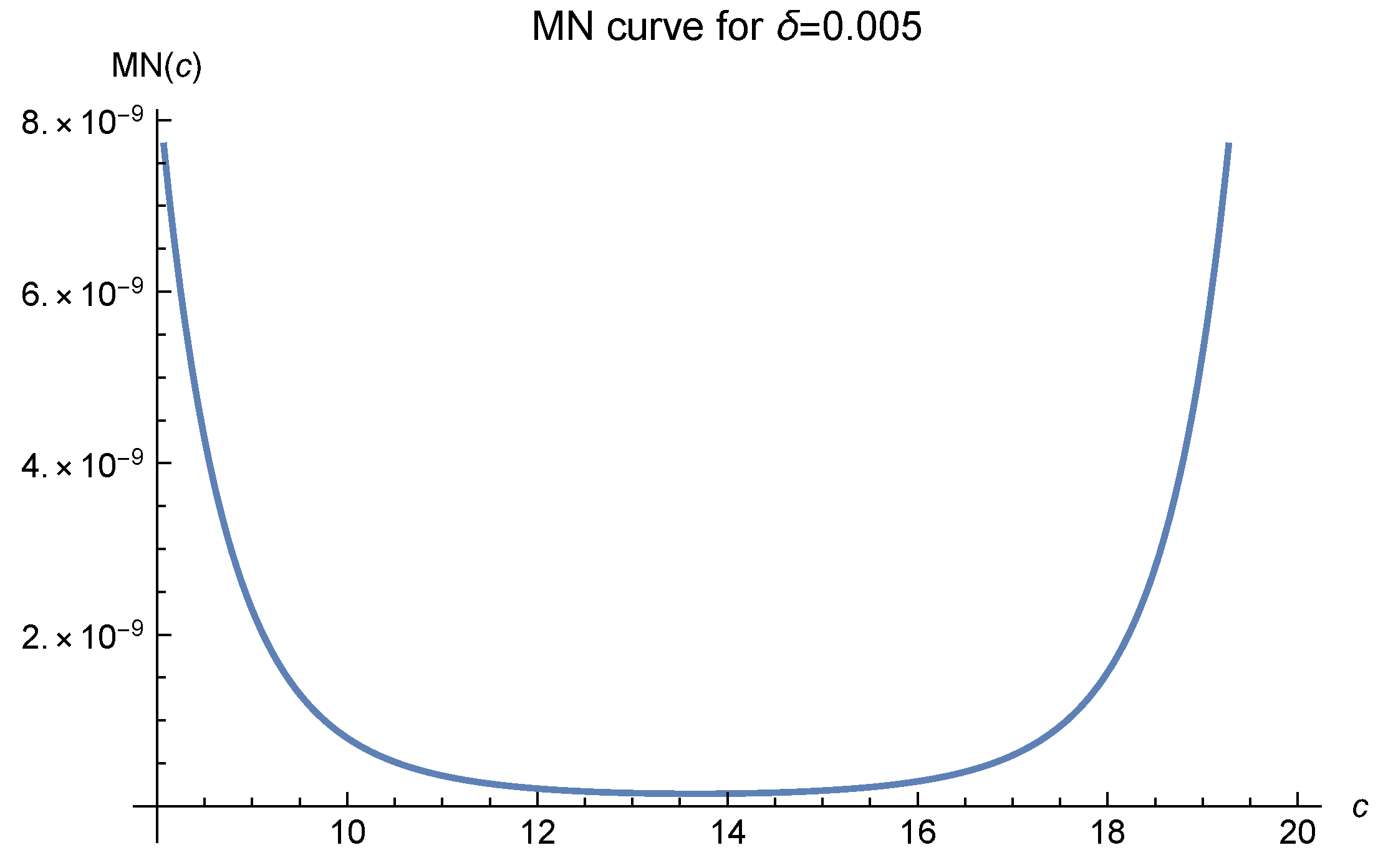
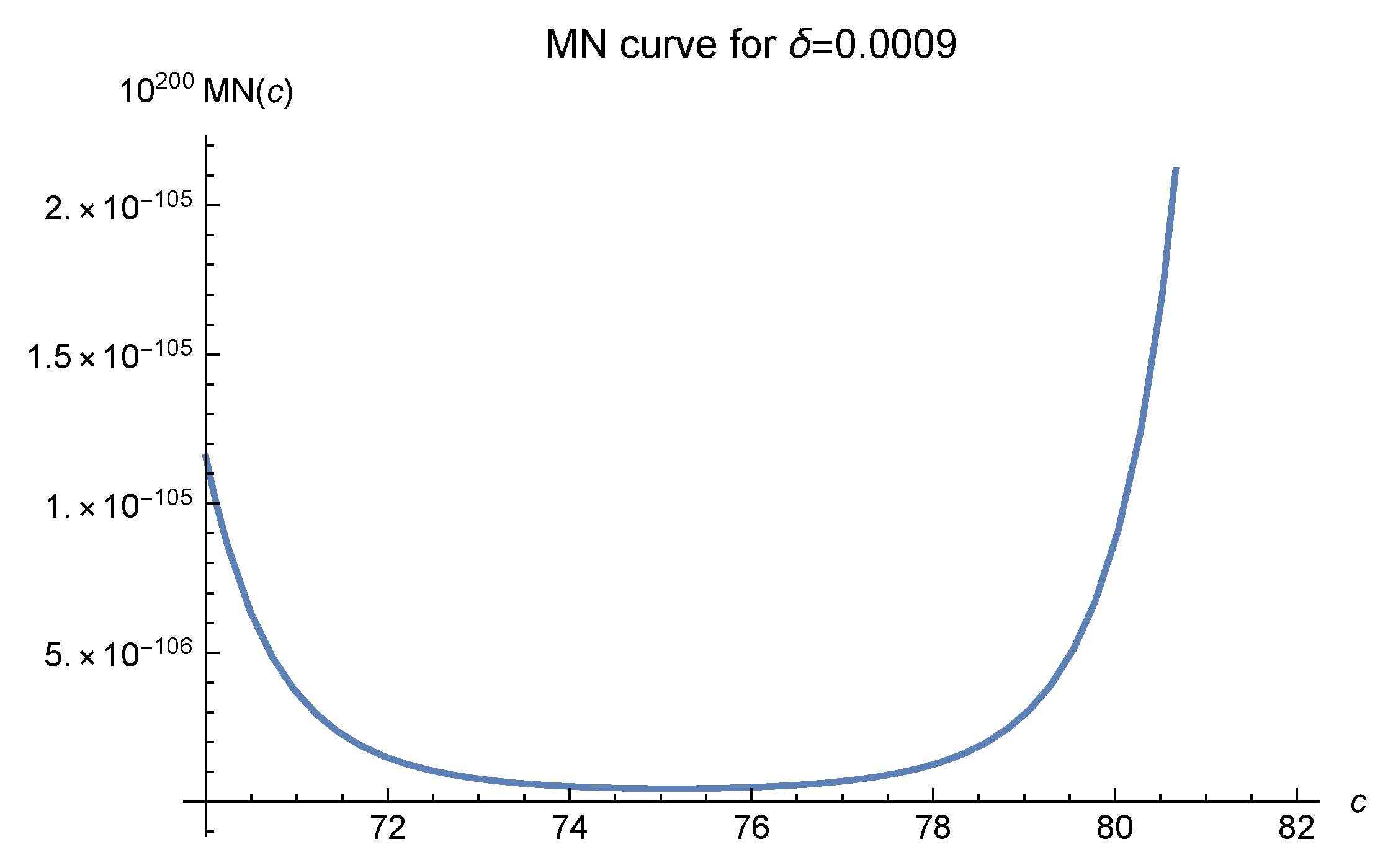
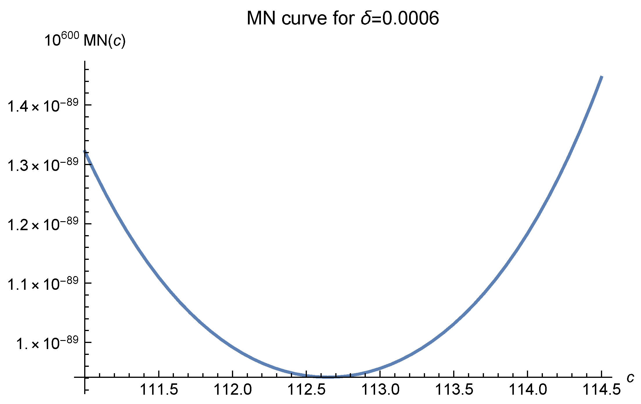
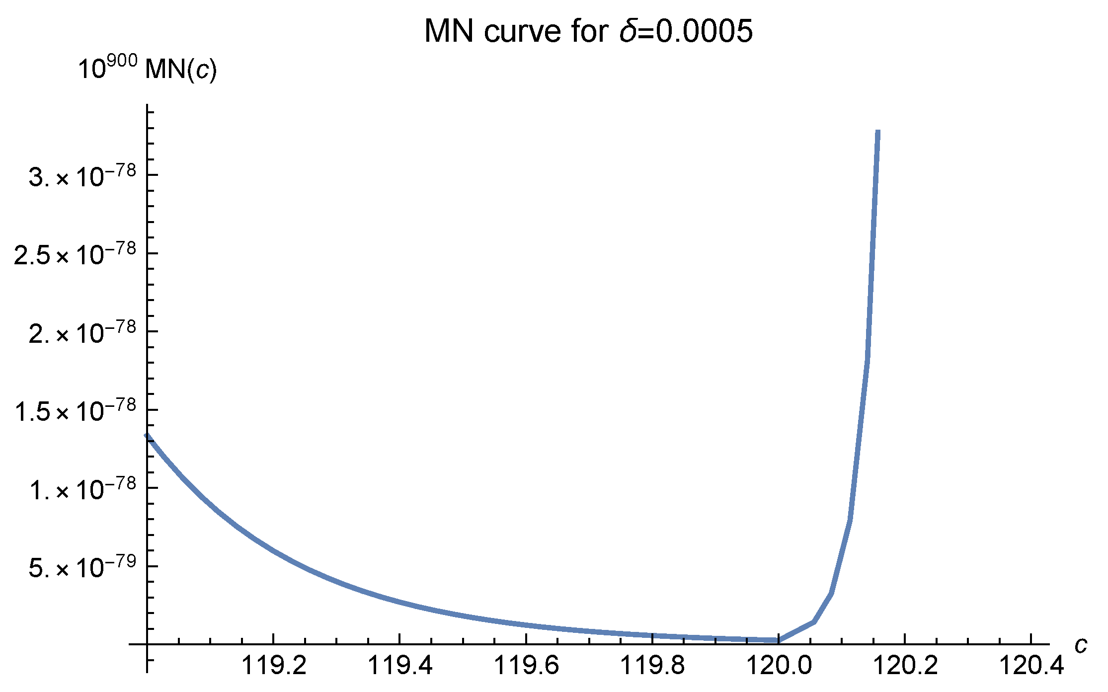
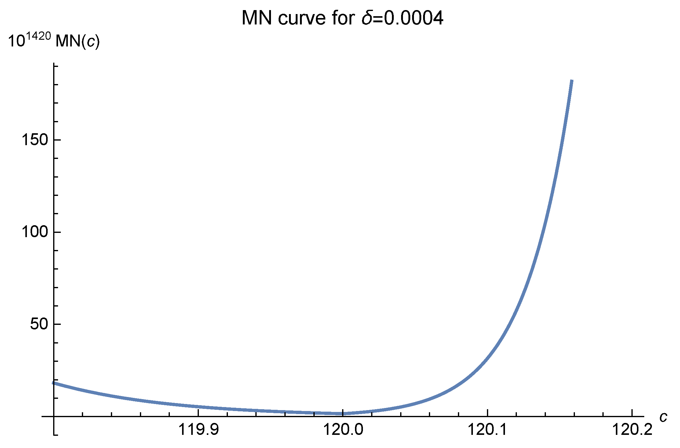
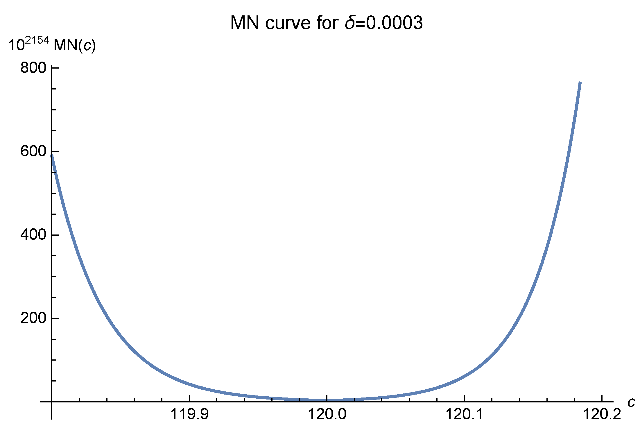
in the domain . Then, , and the MN curves of Case 2 for interpolation apply if we choose . The reason we adopt the inverse multiquadrics is that their programming is easier because the polynomial in (2) disappears. For , where exists, the way of dealing with interpolation for functions can be seen in Luh [2]. We offer six MN curves in Figure 1, Figure 2, Figure 3, Figure 4, Figure 5 and Figure 6, which serve as the essential error bounds for the function interpolations. The number , which greatly affects the MN curves, denotes the diameter of the interpolation domain. In these figures, it is easily seen that as the fill distance decreases, i.e., the number of data points increases, the optimal values of c move to 120 and are fixed there at last. The empirical results, as shown in Luh [12], show that one should choose to make the approximation.
Now, we let
where , and require that satisfies
and
where and for .
This is a standard collocation setting. The function is used to approximate the exact solution of the differential equation. After solving the linear equations for , we test at 400 test points evenly spaced in and find its root-mean-square error (RMS)
The condition number of the linear system is . With the arbitrarily precise computer software Mathematica, we kept 800 effective digits to the right of the decimal point for each step of the calculation, successfully overcoming the problem of ill-conditioning. The computer time for solving the linear system is less than one second. We did not test smaller fill distances and different because the RMS is already satisfactory.
Note that, here, is in the same form as the interpolating function defined in (2) where because . Although the collocation points are not exactly the interpolation points, they are in spirit like the interpolation points. It is not surprising that is very small.
3.2. Two-Dimensional Experiment
Here, the solution function is where . The domain is a large square with vertices , and . The function satisfies
for in the interior of the domain and
for on the boundary .
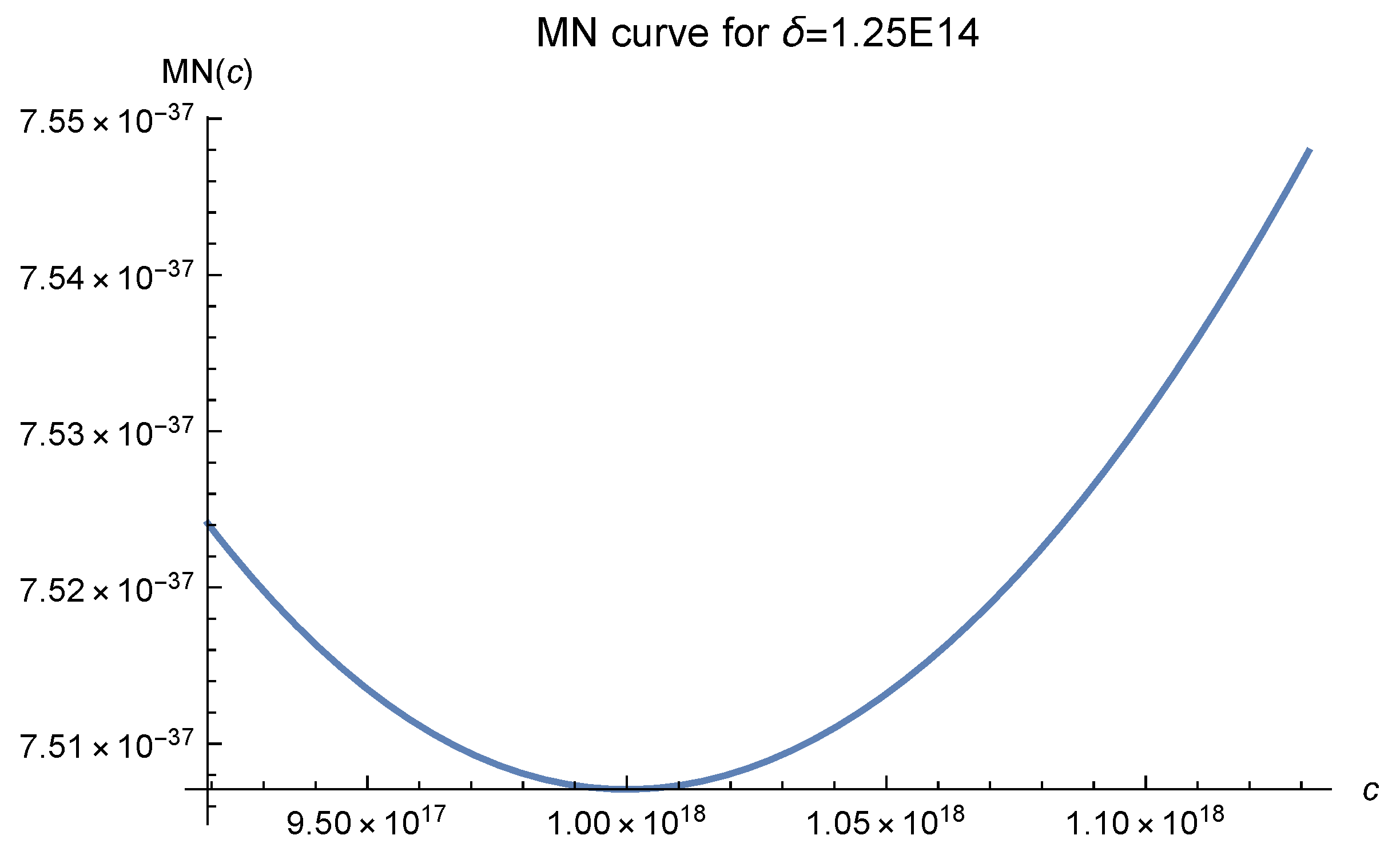
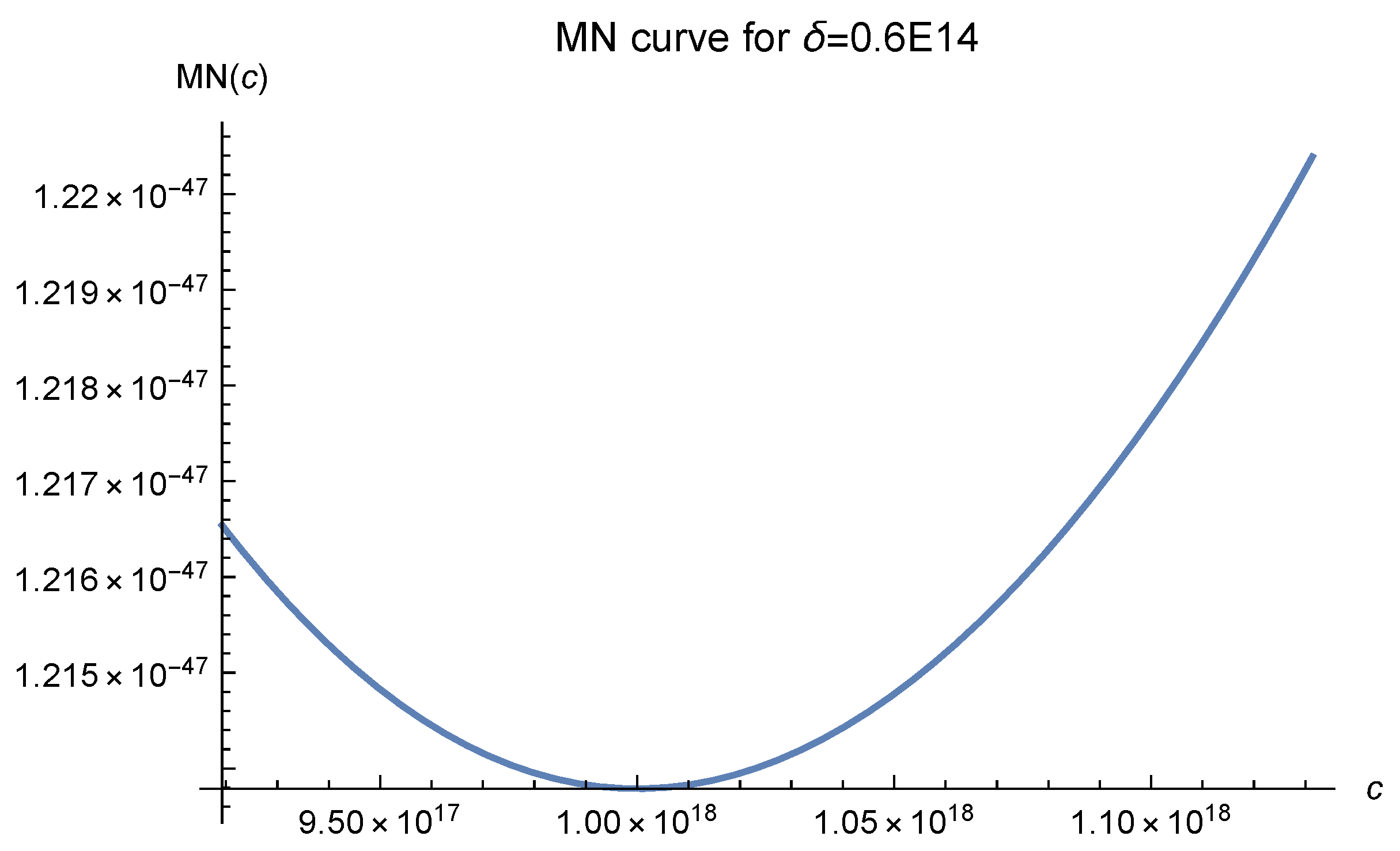
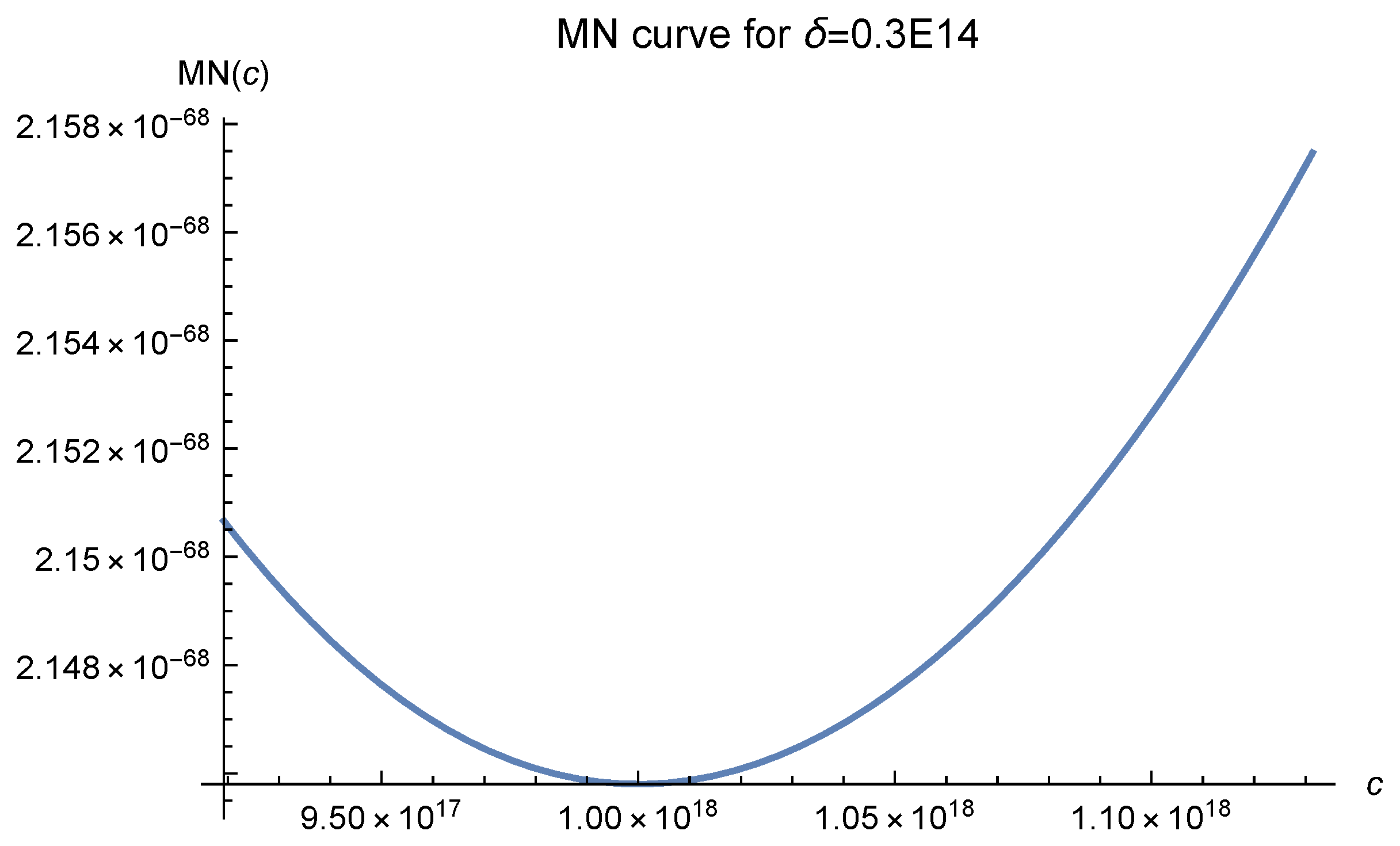
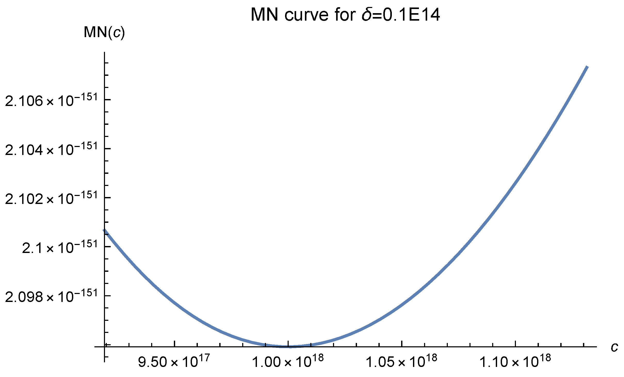
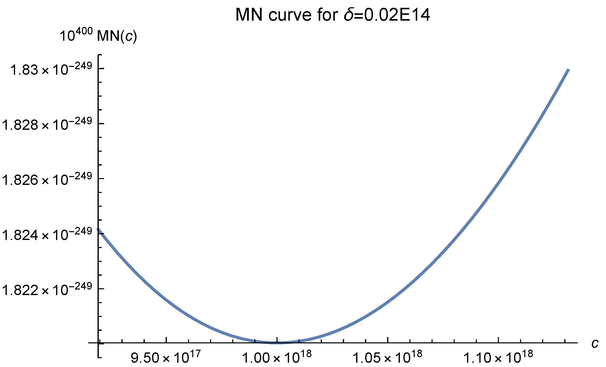
It can be easily checked that where and Case 1 of the MN curves applies if we choose . Five MN curves are shown in Figure 7, Figure 8, Figure 9, Figure 10 and Figure 11.
All these curves show that one should choose as the shape parameter in . We let be the approximate solution of the Poisson equation satisfying (5) and (6), and require that it satisfy
for where belong to the interior of , i.e., , and denotes the number of data points used. Moreover,
for where belong to the boundary .
A grid of is adopted. Hence, there are 1681 data points altogether. Among them, 160 are boundary points where the Dirichlet condition occurs. Thus, the fill distance is E14. The reason we choose such a delta is that it is close to the one in Figure 7. When applying the MN curves, we consider all the 1681 data points to be the interpolation points, even though it is not theoretically rigorous. As explained in Luh [12], it is supposed to work well. However, something important must be pointed out. Although MN curves can be used to predict almost exactly the optimal value of c for function interpolation, a moderate search may be needed if this approach is used in a non-rigorous way. We begin with the theoretically predicted optimal value and test two nearby values, one larger and the other smaller. Then, we check the RMS on the boundary for each c and choose the direction which makes the RMS smaller. Continuing to choose c in this direction, we stop when the RMS values begin to grow. Our experiment shows that not many steps are needed, and the finally obtained c does produce the best result.
The experimental results are presented in Table 1. Here, and denote the root-mean-square error, number of data points, number of test points, and condition number of the linear system, respectively. The optimal value of c is marked with the symbol *. We use to denote the root-mean-square error of the approximation on the boundary, generated by 800 test points located on the boundary. In the entire domain , 6400 test points were used to generate the s. The most time-consuming command of solving the system of linear equations took about 30 min for each c. Although we adopted 1200 effective digits for each step of the calculation, it still worked with an acceptable time efficiency.
Note that the optimal value of c is which coincides with the value chosen by our stopping criterion based on . This optimal value was obtained without much effort. The most time-consuming step is solving a linear system for each trial of the c value whenever the condition number is very large. Fortunately, it took only 30 min in our experiment. Obviously, we could have obtained better RMS values by increasing the number of data points, whereas we did not do so because the approximation was already quite good. Moreover, it can be seen that the theoretical value is not the same as the experimental value. The main reason is that we relaxed two strict requirements in Luh [1,2], as explained in the paragraph preceding Definition 2.2. Another important reason is that, according to the strict theory in [1,2], the MN functions are defined only for function interpolation, not for the collocation method of solving PDEs.
In this paper, all the calculations were not performed by double precision. Instead, they were made by the arbitrarily precise computer software Mathematica. In the MN-curve approach, the condition number of the linear system may be very large. If double precision is adopted, the final results may be meaningless. For example, in Table 1, when , the condition number is . One has to adopt at least 750 effective digits to the right of the decimal point for each step of the calculation. In order to increase the reader’s confidence, we adopted 1200 digits at the cost of spending more time. Hence, our calculations should be reliable. This is about the stability. As for the convergence, in Figure 1, Figure 2, Figure 3, Figure 4, Figure 5, Figure 6, Figure 7, Figure 8, Figure 9, Figure 10 and Figure 11, it can be clearly seen that as the fill distance decreases, the value of MN(c), which denotes the essential error bound of the approximation, decreases rapidly. It fully reflects a salient characteristic of the RBF approach. In our experiments, we did not test different fill distances because our primary concern is finding a good c value, not the convergence rate.
Seemingly, it is a limitation of our approach that one has to adopt Mathematica rather than the widely used Matlab. In fact, it probably can be considered to be a limitation of the entire RBF approach. In Madych [7], an incomplete experiment was presented. Meaningless results appear in that experiment whenever the condition number is greater than . What Madych used was Matlab and a double-precision scheme. In the paper, Madych said that he did not know how to overcome this trouble. By virtue of Mathematica, we can now handle it successfully. The severe ill-conditioning of the RBF approach seems to be an inherent problem which we have to face.
4. Discussion
The author believes that only a very small part of the PDE problems has been dealt with in this paper. For future research, we should try to explore different boundary conditions, different domains, and various PDEs. These will be an endless work.
Another paper by Oaxaca-Adams et al. [13] may be worth mentioning. In [13], a curve is also used to obtain the optimal point of interest, and in a similar way, a numerical approach is used that allows numerically solving a type of systems of interest in applied sciences.
In physics, as said by Kansa, many numerical solutions to PDEs are not bad, but truly good solutions are rarely seen. E. Kansa invented the collocation method and opened a new route to solving them. The combination of the c theory and collocation does produce very good results, as shown in our experiments. Maybe this is just a starting point. We are still facing a huge challenge and have a lot of work to conduct in the future.
Funding
This research was funded by National Science and Technology Council through the MOST project 107-2115-M-126-005. The APC was included.
Institutional Review Board Statement
Not applicable.
Informed Consent Statement
Not applicable.
Conflicts of Interest
The author declares no conflict of interest.
References
- Luh, L.-T. The mystery of the shape parameter IV. Eng. Anal. Bound. Elem. 2014, 48, 24–31. [Google Scholar] [CrossRef] [Green Version]
- Luh, L.-T. The mystery of the shape parameter III. Appl. Comput. Harmon. Anal. 2016, 40, 186–199. [Google Scholar] [CrossRef]
- Kansa, E.J. Multiquadrics—A scattered data approximation scheme with applications to computational fluid dynamics I: Surface approximations and partial derivative estimates. Comput. Math. Appl. 1990, 19, 127–145. [Google Scholar] [CrossRef] [Green Version]
- Kansa, E.J. Multiquadrics-a scattered data approximation scheme with applications to computational fluid dynamics II: Solutions to parabolic, hyperbolic, and elliptic partial differential equations. Comput. Math. Appl. 1990, 19, 147–161. [Google Scholar] [CrossRef] [Green Version]
- Kansa, E.J.; Holoborodko, P. On the ill-conditioned nature of C∞ RBF strong collocation. Eng. Anal. Bound. Elem. 2017, 78, 26–30. [Google Scholar] [CrossRef]
- Powell, M.J.D. Univariate Multiquadric Interpolation: Some Recent Results. In Curves and Surfaces; Academic Press: San Diego, CA, USA, 1991; pp. 371–382. [Google Scholar]
- Madych, W.R. Miscellaneous error bounds for multiquadric and related interpolators. Comput. Math. Appl. 1992, 24, 121–138. [Google Scholar] [CrossRef] [Green Version]
- Rippa, S. An algorithm for selecting a good value for the parameter c in a radial basis function interpolation. Adv. Comput. Math. 1999, 11, 193–210. [Google Scholar] [CrossRef]
- Fasshauer, G. Meshfree Approximation Methods with MATLAB; World Scientific Publishers: Singapore, 2007. [Google Scholar]
- Huang, C.-S.; Lee, C.-F.; Cheng, A.H.D. Error estimate, optimal shape parameter, and high precision computation of multiquadric collocation method. Eng. Anal. Bound Elem. 2007, 31, 615–623. [Google Scholar] [CrossRef]
- Huang, C.-S.; Yen, H.-D.; Cheng, A.H.D. On the increasingly flat radial basis function and optimal shape parameter for the solution of elliptic PDEs. Eng. Anal. Bound Elem. 2010, 34, 802–809. [Google Scholar] [CrossRef]
- Luh, L.-T. The choice of the shape parameter-a friendly approach. Eng. Anal. Bound. Elem. 2019, 98, 103–109. [Google Scholar] [CrossRef]
- Oaxaca-Adams, G.; Villafuerte-Segura, R.; Aguirre-Hernández, B. On nonfragility of controllers for time delay systems: A numerical approach. J. Frankl. Inst. 2021, 358, 4671–4686. [Google Scholar] [CrossRef]
Figure 1.
Here, , and .

Figure 2.
Here, , and .

Figure 3.
Here, , and .

Figure 4.
Here, , and .

Figure 5.
Here, , and .

Figure 6.
Here, , and .

Figure 7.
Here, E16, and E.

Figure 8.
Here, E16, and E.

Figure 9.
Here, E16, and E.

Figure 10.
Here, E16, and E.

Figure 11.
Here, E16, and E.


Table 1.
.
| c | |||||
| c | * | ||||
| c | |||||
Publisher’s Note: MDPI stays neutral with regard to jurisdictional claims in published maps and institutional affiliations. |
© 2022 by the author. Licensee MDPI, Basel, Switzerland. This article is an open access article distributed under the terms and conditions of the Creative Commons Attribution (CC BY) license (https://creativecommons.org/licenses/by/4.0/).
Share and Cite
MDPI and ACS Style
Luh, L.-T. Solving Poisson Equations by the MN-Curve Approach. Mathematics 2022, 10, 4582. https://doi.org/10.3390/math10234582
AMA Style
Luh L-T. Solving Poisson Equations by the MN-Curve Approach. Mathematics. 2022; 10(23):4582. https://doi.org/10.3390/math10234582
Chicago/Turabian StyleLuh, Lin-Tian. 2022. "Solving Poisson Equations by the MN-Curve Approach" Mathematics 10, no. 23: 4582. https://doi.org/10.3390/math10234582
Note that from the first issue of 2016, this journal uses article numbers instead of page numbers. See further details here.