Knowledge Gradient: Capturing Value of Information in Iterative Decisions under Uncertainty

Abstract

Many real-life problems that involve decisions under uncertainty are often sequentially repeated and can be approached iteratively. Knowledge Gradient (KG) formulates the decision-under-uncertainty problem into repeatedly estimating the value of information observed from each possible decisions and then committing to a decision with the highest estimated value. This paper aims to provide a multi-faceted overview of modern research on KG: firstly, on how the KG algorithm is formulated in the beginning with an example implementation of its most frequently used implementation; secondly, on how KG algorithms are related to other problems and iterative algorithms, in particular, Bayesian optimization; thirdly, on the significant trends found in modern theoretical research on KG; lastly, on the diverse examples of applications that use KG in their key decision-making step.

1. Introduction

Decision making under uncertainty is one of the fundamental tasks not only of scientific methods but also of everyday life. Ranging from mundane yet important decisions such as choosing a lunch menu to deciding which variations of hypotheses to test in the next iteration of experiments in academic research, decision making is ubiquitous in human life. The fundamental uncertainty that makes such decision making a challenging task is that every decision results in a corresponding aftermath, which is unknown prior to committing to the decision.

Due to the ubiquity of the problem in the real world, there are many directions in which mathematics is used to handle uncertainty in order to improve or assist overall decision making processes. A notable example is taking multiple criteria into consideration to alleviate subjectivity or bias into decision making, which is found in applications from different fields: ref. [1] presents a method to rank asphalt production plants under multiple decision criteria; ref. [2] applies multiple criteria decision making method in human resource decision of personnel management; ref. [3] designs sustainable measures of mobility by ranking and selecting multiple candidate measures by professionals. To handle uncertainty in subjectivity, this method of decision making can be further extended as follows: ref. [4] uses a fuzzy comparison matrix to model the potential uncertainty of criteria ranking due to subjectivity; ref. [5] incorporates fuzzy sets to represent the uncertainty of relative importance quantification in decision criteria.

Randomness due to subjectivity is not the only uncertainty in the field of decision making. For example, considering the best decision to be the optimal decision that leads to optimizing the key response variable such as profit or income, modeling the innate uncertainty in how decision leads to response is another wide field of applied mathematics. When predicting the monthly income of an online storefront, it is essential to estimate the sales of the store, for which a hidden Markov model can be used to model the customer decision making process that affects the sales [6]. Financial portfolio management has different optimality conditions—often minimizing portfolio variance—and finding the corresponding optimal allocation of assets is a challenging decision making task that must face market uncertainty. To model the uncertainty in the optimal asset allocation problem, ref. [7] presents a latent variable model that uses student’s t-distribution-based stochastic processes instead of the traditional Gaussian process. Estimating risk can be directly modeled by estimating the Value-at-Risk measure, and ref. [8] presents thee Bernstein copula-based method to model the risk measure adaptively. The aforementioned examples are just a few of the mathematical modeling of uncertainty methods, which can be coupled to other optimization tasks to solve real world operations such as reverse stress testing [9].

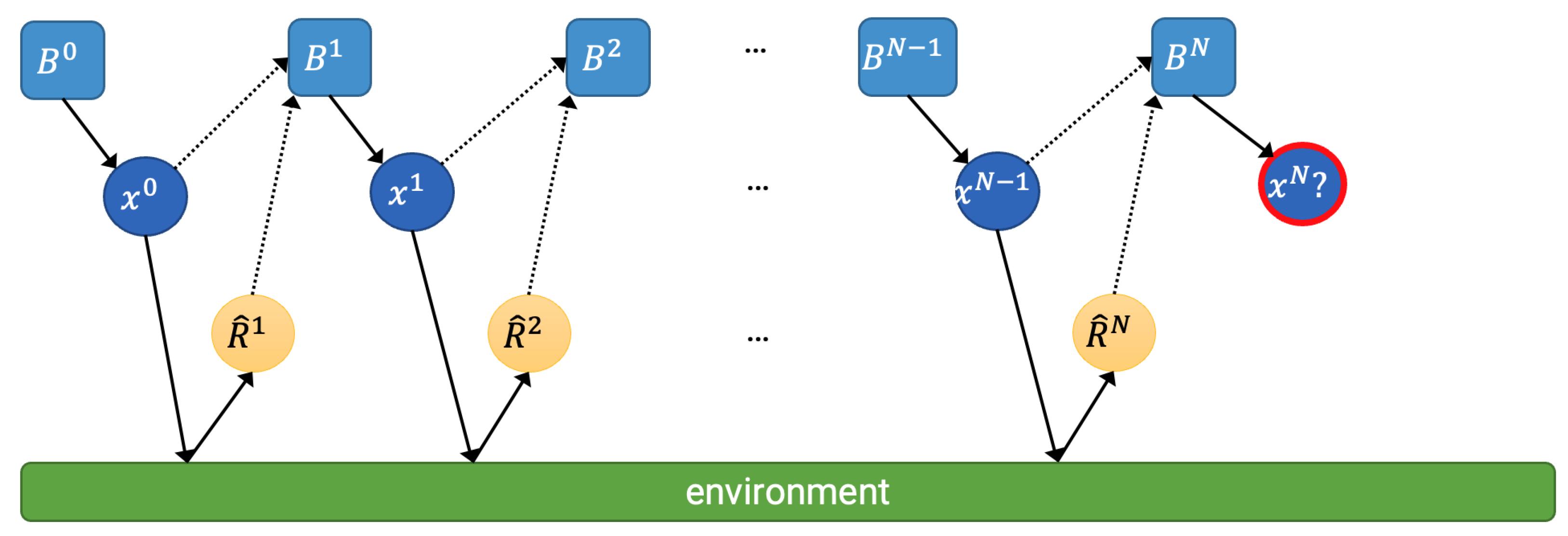
Adding another twist to the situation, in particular, the problem class of interest in this review article is sequential decision making under uncertainty, in which the decision making agent must make a series of decisions. Here, the agent is assumed to be intelligent, in a sense that it will learn from its previous decisions and its aftermath. Note that even if the same decision is repeated multiple times, the observed response may not be the same in value due to the innate uncertainty of the response. Depending on how the decision candidates and the objective function is formulated, sequential decision making problems can be cast into a number of different problems such as ranking and selection (R&S), multi-armed bandit, and Bayesian optimization, to name a few. Here, we focus on emphasizing the essence of the sequential decision problem with Figure 1:

The internal state of the decision-making agent at time n, represented as beliefs ($B^n$) that contain sufficient information to make decision at time n$\left(x^n\right)$, will evolve as the agent observe the resulting “decision–response” pair of $(x^n,{\widehat{R}}^{n+1})$ into $B^{n+1}$, which will contain the newest information extracted from the “decision–response” pair. For such a decision-making agent to learn the environment and find out the optimal decision-making rule, two properties are crucial:

• Learning from the response: learn efficiently from the observed experience.
• Decision making: make effective decisions that lead to learning what is unknown.

A knowledge gradient (KG) algorithm covers both aspects, such that for every time step it (1) learns efficiently with Bayesian inference and (2) makes decisions that maximize the estimated value of information to be learned from the next experience of the “decision–response”. The Knowledge gradient (KG) value of any decision candidate at any time step is a quantification of the aforementioned estimated value of information, which makes KG algorithms readily explained as a rational agent that tries to extract most information from every decision. In the rest of the review article, the following topics of KG algorithms are covered:

• Problem setup and fundamental properties of KG algorithms;
• KG and its related problems, especially Bayesian Optimization (BO);
• Survey on theoretical advances of KG-based algorithms;
• Survey on recent applications of KG-based algorithms.

2. Knowledge Gradient Algorithm

The knowledge gradient (KG) algorithm stands for a class of iterative optimization algorithms that first appeared in [10] and later developed thoroughly in [11] as a principled approach to solve fixed-budget stochastic ranking and selection (R&S) problems. Therefore, the R&S problem formulation will be presented first in Section 2.1, and the knowledge gradient later in Section 2.2.

2.1. Preliminary: Ranking and Selection Problem

R&S problems are defined by a known set of alternatives or possible decisions, and their unknown response values, and solving them requires finding the best decision according to a given objective function. Usually they are formulated as either finding the decision with the largest average response value—seeing the value as benefit or reward—or finding the decision with the smallest average response value—seeing the value as a demerit or cost. In this review, without loss of generality, we choose the maximization formulation that assumes the response values are considered as rewards, and the objective function formulated to maximize the expected reward naturally aligns with finding the optimal decision. Hence, an algorithm that solves an R&S problem must find the best decision through trial and error, as the intrinsic values of the decisions are initially unknown and must be estimated by observations revealed through choosing the corresponding decisions. Fu and Henderson [12] provide a historical discourse and Hong et al. [13] provide a categorical discourse on R&S problems.

There are many problems that are related to R&S problems, such as the best arm identification problem, budget allocation problem, multi-armed bandit (MAB) problem, and Bayesian optimization. The formulations and notations used in each of the related problems are not always compatible with each other. So in this review, we first introduce the minimal notations to formulate the R&S problem class solved by the first KG algorithm [11].

Let the set of decisions be $\mathcal{X}$, whose elements x’s are distinct alternatives or decisions. For now, assume the number of alternatives to be finite, i.e., $\left|\mathcal{X}\right|<\infty$. We also assume that the time horizon T is given, which means that the maximum number of decisions can be made in the given R&S problem is finite and known before any decision is made. Time index variable $t=0,1,\cdots ,T-1$ is used to index variables, such as the decision made at time t as $x_t$. Upon choosing a decision x, a reward corresponding to that decision is observed, and we assume a stochastic R&S problem, such that the true stationary distribution $R\left(x\right)$, which the reward follows, is unknown to the decision-making agent. Therefore, an R&S problem can be stated as an optimization problem whose objective function is:

$$\begin{array}{c}\hfill \underset{x_T\in \mathcal{X}}{max}\mathbb{E}\left[R\left(x_T\right)|R\left(x_0\right),R\left(x_1\right),\cdots ,R\left(x_{T-1}\right)\right],\end{array}$$

(1)

within the finite budget T to sample the random variables $R\left(x_0\right),R\left(x_1\right),\cdots ,R\left(x_{T-1}\right)$ by choosing $x_0,x_1,\cdots ,x_{T-1}$ from $\mathcal{X}$.

The reward of choosing $x_t$ is observed immediately, in a sense that it is observed before making another decision at time $t+1$. Note that the time index t captures the time between the last decision $x_{t-1}$ beinig made and the moment the t-th decision is made, such that the response observed by $x_t$ is indexed with $t+1$ as ${\widehat{R}}_{t+1}$. Furthermore, an additive intrinsic stochasticity or noise of observation is assumed, such that a zero-mean Gaussian random variable $ϵ\sim \mathcal{N}\left(0,{\sigma }_{ϵ}\right)$ is added to the noiseless observation $R\left(x_t\right)$ for all $x,t$. Hence, the observed response ${\widehat{R}}_{t+1}$ from choosing decision $x_t$ at time t, satisfies the following:

$$\begin{array}{c}\hfill {\widehat{R}}_{t+1}=R\left(x_t\right)+ϵ.\end{array}$$

(2)

The parameter ${\sigma }_{ϵ}$ expresses the intensity of the intrinsic noise $ϵ$, and this is assumed to be known to the agent a priori. The introduction of such $ϵ$ may be seen as introducing the following assumptions: (1) $ϵ\sim \mathcal{N}\left(0,{\sigma }_{ϵ}\right)$ means that the agent is certain of the unbiasedness of the measurement, i.e., no systematic bias is introduced due to intrinsic noisy measurement, and (2) knowing ${\sigma }_{ϵ}$ a priori means that the agent is aware of the precision or the resolution of its own sensor that measures the observation.

2.2. KG: Capturing Value of Information in R and S Problems

The first knowledge gradient algorithm [11] is called KG with the independent Gaussian belief model, which clarifies that the “belief” on the distribution of $R\left(x\right)$ for each $x\in \mathcal{X}$ can be modeled by $\left|\mathcal{X}\right|$ independent Gaussian distributions, each with unknown mean parameter ${\mu }_x$ and standard deviation ${\sigma }_x$. Belief state at time t, denoted as $B_t$, contains $\overrightarrow{\mu }$ and $\overrightarrow{\sigma }$, which are $\left|\mathcal{X}\right|$-dim real vectors with elements corresponding to estimates of means and standard deviations at time t. Note that $B_t$ must contain sufficient information to precisely describe the “belief” in the model of the the current time, t, and reward for each and every decision. Withstanding a little abuse of notation, we assume that conditioning on $B_t$ provides not only the parameter values that are explicitly given but also the implicit modeling detail such as the distribution type. Every knowledge gradient algorithms have a particular belief model and additional assumptions, and many different possible belief models are explained in greater detail in [14]. In this article, we focus our discussion on KG with the independent Gaussian belief model, as (1) it provides a theoretical foundation for more complicated KG algorithms and (2) it is the most frequently used KG algorithm in recent applications.

We define the value of information in R&S problems gathered up to time t as the largest expected reward, when the subsequent decision $x_t$ is made to maximize the corresponding reward. Therefore, we can use conditional expectation as follows:

$$\begin{array}{c}\hfill V_t:=\underset{x\in \mathcal{X}}{max}\mathbb{E}\left[R\left(x\right)|B_t\right],\end{array}$$

(3)

where $B_t$ is the belief state at time t. Comparing the value of information to the objective function of the R&S problem shown in Equation (1), it becomes obvious that $B_t$ is defined to encode all the past information $R\left(x_0\right),\cdots ,R\left(x_{t-1}\right)$ to solve the R&S problem objective function at any time $t\le T$.

Note that the choice of the belief model in the KG algorithm will determine how the value can be evaluated from the information in belief state $B_t$. Therefore, the belief state $B_t$ can be seen as a model-specific representation of information gathered up to time t in the R&S problem to compute $V_t$ at any time t. Particularly, in KG with the independent Gaussian belief model, where $R\left(x\right)\sim \mathcal{N}({\mu }_x,{\sigma }_x)$ by modeling assumption, computing $V_t$ becomes simply finding the maximal among the corresponding parameters from the given belief state $B_t=\left\{\overrightarrow{\mu },\overrightarrow{\sigma }\right\}$ as:

$$\begin{array}{cc}\hfill V_t& :=\underset{x\in \mathcal{X}}{max}\mathbb{E}\left[R\left(x\right)|B_t\right]\hfill \end{array}$$

(4)

$$\begin{array}{cc}\hfill & =\underset{x\in \mathcal{X}}{max}\left\{{\mu }_{1,t},\cdots ,{\mu }_{\left|\mathcal{X}\right|,t}\right\},\hfill \end{array}$$

(5)

since $\forall x\in \mathcal{X}:\mathbb{E}\left[R\left(x\right)|B_t\right]={\mu }_{x,t}$ at any t.

At any time t for any decision $x\in \mathcal{X}$, its KG value, denoted ${\nu }_x$, can be defined as the following conditional expectation:

$$\begin{array}{c}\hfill {\nu }_t\left(x\right):=\mathbb{E}\left[V_{t+1}-V_t|B_t,x_t=x\right],\end{array}$$

(6)

where $x_t=x$ denotes the conditional event of “assuming the agent makes the current decision $x_t$ to be x”. The standard interpretation of ${\nu }_t\left(x\right)$, the KG of decision x, is the expected improvement of value by observing another feedback of choosing decision x [15]. Note that the conditional expectation in Equation (6) is with respect to random variable $V_{t+1}$.

Particularly, when the belief model contains a parameter representing the expected reward $R\left(x\right)$ given x at time t, such as ${\mu }_{x,t}$ in independent Gaussian belief model, Equation (6) can be further simplified as:

$$\begin{array}{cc}\hfill {\nu }_t\left(x\right)& :=\mathbb{E}\left[V_{t+1}-V_t|B_t,x_t=x\right]\hfill \end{array}$$

(7)

$$\begin{array}{cc}\hfill & =\mathbb{E}\left[{\mu }_{x,t+1}-{\mu }_{x,t}|B_t,x_t=x\right]\hfill \end{array}$$

(8)

$$\begin{array}{cc}\hfill & =\mathbb{E}\left[{\mu }_{x,t+1}|B_t,x_t=x\right]-{\mu }_{x,t}.\hfill \end{array}$$

(9)

Note that Equation (9) explicitly shows the one-step look-ahead behavior of KG, which requires computing the conditional expectation of what the belief state ${\mu }_x$ will be at time $t+1$, given information at time t and decision x. As clearly shown above, the knowledge gradient ${\nu }_t\left(x\right)$ can be interpreted as the expected improvement of the average reward of choosing x at t, assuming additional information is obtained from decision x at time t is modeled from belief state $B_t$.

2.3. Decision Making Step in KG Algorithm

At each time t, a KG algorithm computes ${\nu }_t\left(x\right)$ for all decisions $x\in \mathcal{X}$ and makes decision at time t as:

$$\begin{array}{c}\hfill x_t=arg\underset{x\in \mathcal{X}}{max}\left\{{\nu }_t\left(x\right)\right\},\end{array}$$

(10)

which is to choose the decision x that has the largest KG value ${\nu }_t\left(x\right)$. Hence, the KG algorithm requires an explicit method to compute ${\nu }_t\left(x\right)$ for any $t,x$, given $B_t$, and the method may differ from the belief model assumed by the algorithm.

In particular, with the independent Gaussian belief model, it is possible to efficiently compute ${\nu }_t\left(x\right)$ for any decision $x\in \mathcal{X}$

$$\begin{array}{c}\hfill {\nu }_t\left(x\right):={\sigma }_{\nu }\left({\xi }_{x,t}\Phi \left({\xi }_{x,t}\right)+\varphi \left({\xi }_{x,t}\right)\right),\end{array}$$

(11)

where $\Phi (·)$ and $\varphi (·)$ are the cumulative distribution function and the probability density function of standard Gaussian distribution, respectively, and ${\xi }_{x,t}$ is defined as:

$$\begin{array}{c}\hfill {\xi }_{x,t}:=-\left|\frac{{\mu }_{x,t}-{max}_{x^{\prime }\ne x}{\mu }_{x^{\prime },t}}{{\sigma }_{\nu }}\right|,\end{array}$$

(12)

where ${\mu }_{x,t}$ is the mean parameter of the reward distribution of decision x estimated at time t (as part of the belief state $B_t$), and ${\sigma }_{\nu }$ is defined as:

$$\begin{array}{c}\hfill {\sigma }_{\nu }:=\frac{{\sigma }_{x,t}}{\sqrt{1+{\left(\frac{{\sigma }_{ϵ}}{{\sigma }_{x,t}}\right)}^2}},\end{array}$$

(13)

where ${\sigma }_{x,t}$ is the standard deviation parameter of the reward distribution of decision x estimated at time t (as part of the belief state $B_t$).

Two important theoretical properties of KG with independent Gaussian belief algorithm are as follows [16]:

• Makes a myopically optimal choice, such that if the current decision is the last decision to make in an R&S problem, the decision based on the KG algorithm is the optimal choice.
• Finds optimal choice asymptotically, such that if the KG algorithm is followed, it is always guaranteed to find the optimal decision among finite $\mathcal{X}$ after learning from a finite number of decisions.

The first property is due to the fact that the knowledge gradient of a decision is the expected improvement of best reward after seeing one more result from the decision. This is an immediate corollary from Equations (6) and (10). The second property is due to the fact that the knowledge gradient is guaranteed to sample each decision frequently enough to overcome finite random bias introduced by stochasticity. Proof of this property needs discussion on the learning step of the KG algorithm, found in Section 2.4.

2.4. Learning Step in KG Algorithm

When a decision $x_t$ is made and the corresponding result ${\widehat{R}}_{t+1}$ is observed, the agent following the KG algorithm must update their belief state $B_{t+1}$ to reflect the new set of information: decision $x_t$ and the incurred result ${\widehat{R}}_{t+1}$. Let the space of belief states be $\mathcal{B}$. For example, the belief state of KG with independent Gaussian belief model can be stated as $\mathcal{B}={\mathbb{R}}^{\left|\mathcal{X}\right|}\times {\mathbb{R}}_{+}^{\left|\mathcal{X}\right|}$, where ${\mathbb{R}}_{+}:=\left\{x\in \mathbb{R}|x\ge 0\right\}$, since the belief state is comprised of $\left|\mathcal{X}\right|$ parameters for the means and $\left|\mathcal{X}\right|$ parameters for the standard deviations of the reward distribution for each possible decision. The first batch of research papers on KG [16,17,18,19] uses $S^M:\mathcal{B}\times \mathcal{X}\times \mathbb{R}\to \mathcal{B}$, named “state model”, to designate the function that maps the old belief state to the new belief state given a new set of information. The name “state model” implies that $S^M$ the “(transition) model” of the “state” of KG algorithm at any time t; and it may be understood as the transition functional of belief states, which requires the information pair $\left(x_t,{\widehat{R}}_{t+1}\right)$ at any t to actually become the function that maps the current belief state $B_t$ to the next belief state $B_{t+1}$.

As the belief state is derived from the belief model, the form of $S^M$ and the availability of a closed-form formula depends on the belief model used in the KG algorithm. For example, in KG with independent Gaussian belief, $S^M$ can be stated in a closed form formula for each of the belief state parameters. First, given $x_t$, its response $\widehat{R}\left(x_t\right)$, and the belief state $B_t=\left\{\overrightarrow{\mu },\overrightarrow{\sigma }\right\}$ at time t, the updated standard deviation parameter ${\sigma }_{x,t+1}$ can be computed as:

$$\begin{array}{c}\hfill {\sigma }_{x,t+1}=\sqrt{\frac{{\sigma }_{x,t}^2}{1+\frac{{\sigma }_{x,t}^2}{{\sigma }_{ϵ}^2}}},\end{array}$$

(14)

and the updated mean parameter ${\mu }_{x,t+1}$ as:

$$\begin{array}{c}\hfill {\mu }_{x,t+1}={\sigma }_{x,t+1}^2\left(\frac{{\mu }_{x,t}}{{\sigma }_{x,t}^2}+\frac{\widehat{R}\left(x_t\right)}{{\sigma }_{ϵ}^2}\right).\end{array}$$

(15)

2.5. Modeling Belief and Reward in KG Algorithms

The fundamental setup of KG algorithms and its particular realization under the independent Gaussian belief model has been the topic up to this point. We take a step back, and consider an even more fundamental question: how the problem to be solved can affect the belief model of KG algorithms. Let us assume that a problem to be solved can be cast as an R&S problem. To use a KG algorithm to solve the R&S problem, there is an important design decision that must be made as soon as possible—how to decide the distributions of the belief of the algorithm and the response of the R&S problem. Fundamentally, this is a modeling decision that is ultimately dependent on whether the original problem specification is compatible with the modeling, yet there is another compatibility issue between the modeled problem and the KG algorithm to be used.

First of all, the response $R\left(x\right)$ for $x\in \mathcal{X}$ should be compatible to the problem to solve. The Gaussian response works well in many cases where the unknown response to each decision can be safely assumed as a Gaussian random variable with unknown mean and variance. However, there are situations where this assumption is not compatible. For example, when the response is known to be binary, such that the response to the decision may be either positive or negative, the KG algorithm with the Beta–Bernoulli belief model is a more natural fit with the problem than the KG algorithm with a Gaussian belief model. A handful of methods to compute KG with different belief models exist, as listed on

Table 1. KG belief models with closed-form update rule and KG computation formula, corresponding to the response types.

Response Type	Response Distribution	KG Belief Model
Continuous (Independent)	Gaussian	Independent Gaussian Belief Model
Continuous (Correlated)	Gaussian	Correlated Gaussian Belief Model
Binary	Bernoulli	Beta–Bernoulli Belief Model
Positive Continuous	Exponential	Gamma–Exponential Belief Model
Positive Discrete	Poisson	Gamma–Poisson Belief Model
Bounded Continuous	Uniform	Pareto–Uniform Belief Model

, based on their response variable types.

Computing $S^M$ efficiently has a significant practical impact on any KG algorithm since every consecutive decision $S^M$ needs to be computed, as it captures how to learn from the information pair $\left(x_t,{\widehat{R}}_{t+1}\right)$ and encodes what is learned into the belief state $B_{t+1}$. Therefore, most KG algorithms pay extra attention to establish a tractable computation method to update the belief state $B_t$ to $B_{t+1}$. In particular, all KG algorithms in Table 1 have a closed-form update rule, explained in more detail in Chapter 2 of [14], whose derivation originates mainly from the rich theory of conjugate priors in Bayesian inference. For example, the update rules for belief states in KG with independent Gaussian belief, for each decision $x\in \mathcal{X}$, is the same as the posterior predictive parameter update formula in Bayesian inference with 1-dimensional Gaussian priors and 1-dimensional Gaussian likelihood distribution.

Furthermore, all KG algorithms in Table 1 have closed-form KG computation rule, explained in more detail in Chapter 4 of [14]. Yet, as reviewed in the later section of this review, most applications report that Gaussian belief models are effective in real world problem solving, perhaps due to Central Limit Theorem allowing the sample mean of a wide range of distributions converge to a Gaussian limiting distribution.

A number of important modeling characteristics of KG algorithms arise from how KG algorithms utilize Bayesian inference can be summarized as follow:

• Despite the canonical freedom to choose the true distribution of $R\left(x\right)$ given decision x, the choice is often affected by the availability of conjugate Bayesian priors.
• If a conjugate prior distribution is available, it can be used as the belief model to have the corresponding state space $\mathcal{B}$ valid for all t, which is derived from the theory of conjugate priors in Bayesian inference.
• With the conjugate prior distribution used as the belief model, there exists a closed form formula that can be used as the update rule $S^M$.
• In practice, Gaussian belief models are most frequently used variant of KG algorithms, as a wide range of random variables converge to Gaussian according to the Central Limit Theorem.

3. How KG Relates to Other Algorithms

The KG algorithm started as a solution to thee R&S problem, which can be seen as a constrained optimization of finding, which of a set of unknown stochastic response variables $R\left(x\right)$’s, has the largest expectation via iterative choice of T sequential decisions $x_0,x_1,\cdots ,x_{T-1}$ from a predefined decision space $\mathcal{X}$. Problems that share similar characteristics were found in several different fields, formulated with different set of assumptions, and resulted in several different classes of algorithms that solve the respective formulation of the problems. In this section, we will note several classes of problems that are closely related to the KG algorithm, and in particular, take a deeper look into Bayesian optimization.

The response surface method (RSM) was introduced in the early 1950s [20], with the aim of finding the explanatory variable values that achieve optimal response from an experiment through a sequence of trial and errors. Considering the computational capacity of the era, RSM uses second-order polynomials as a surrogate function to model the response function, and assumes independence among the explanatory variables. RSM is still used in different fields such as manufacturing optimization [21] and chemical plants [22] since the method explicitly aims to find the optimum of an unknown response surface, despite its strong assumptions on the surrogate model. A more detailed survey on RSM can be found in a historical setup [23] and a modern perspective [24].

Kriging is another method popularized in the field of geostatistics and earth scientists since the mid-1960s [25]. It provides a statistically well-founded infilling method to reconstruct the entire surface of function from a finite set of observed samples from the function. Based on a different set of modeling assumptions, there are many types of kriging, such as ordinary kriging, simple kriging, and universal kriging. The theoretical foundation of most kriging methods can be traced back to Gaussian process (GP) regression and Best Linear Unbiased Prediction (BLUP) [26]. A more detailed comparison of different versions of kriging methods can be found in [27].

Efficient Global Optimization (EGO), proposed in [28] as a general purpose optimization algorithm, embeds the essence of the kriging method into a larger framework that is later called Bayesian optimization. EGO succinctly captures the idea of kriging to use Gaussian processes as a surrogate function, which has desirable asymptotic properties from a Bayesian statistics perspective. In particular, EGO introduces Expected Improvements (EI) as the acquisition function, which determines the input to use to measure the objective function, such that following the acquisition function will efficiently optimize an expensive-to-measure black box objective function in an iterative manner. The original formulation of EGO did not handle stochastic or noisy measurements, but later [29] extends EGO to build Sequential Kriging Optimization (SKO), which can handle stochastic black box functions. More detailed advancement on sequential Kriging-based methods can be found in [30].

The three methods—RSM, kriging, EGO—share a common interest in optimizing over an unknown function via iterative sampling. However, the three methods have distinctive characteristics: RSM is explicit in finding the optimum of the unknown function using simpler surrogate functions, whereas kriging methods aim to minimize variance over the entire function domain using Gaussian processes, and EGO distinctively emphasizes the efficiency of using less sampling to find the optimum of the unknown function.

3.1. KG and Bayesian Optimization

Bayesian optimization (BO) [31], which gained attention along with EGO [28] and even more popularity with its application to optimizing deep neural networks [32], is another iterative algorithm that finds the global optimum of black-box functions. Almost, if not every, implementation of BO algorithms uses Gaussian processes as its statistical foundation to model the unknown function whose optimum point is to be found. Hence, it is a valid viewpoint to consider BO as a method that uses surrogate functions, such as RSM, but of tighter ties to statistics to support the asymptotic properties required for modern machine learning. Gaussian process regression, to be precise, is the main learning process when BO uses the Gaussian process as a surrogate function. A thorough exposition on how Gaussian process can be used in machine learning can be found in [33].

BO algorithms have a prototypical structure shared by almost all of their variants. We present the prototypical BO algorithm in

Table 2. Algorithmic structure of a prototypical Bayesian optimization solving R&S problems.

Prototypical BO Algorithm

1:  Initialize Gaussian process prior using B0 (injecting the modeling assumptions) 2:  for t < T do 3:        Choose next decision $x_t\in \mathcal{X}$ according to a predefined acquisition function 4:        Observe a new data $R_{t+1}\sim R\left(x_t\right)$ 5:        Update the posterior $B_{t+1}$ using all available data 6:        Increase t 7:  Return ${\arg max}_{x\in \mathcal{X}}\mathbb{E}\left[R\left(x\right)|B_T\right]$ using the final posterior BT

, using the modeling convention from the R&S problem and KG algorithm to highlight high-level similarity between the KG algorithm and BO algorithm.

A deeper discussion on the theory and application of BO can be found in a series of recent reviews: ref. [34] is a review of BO from the perspective of machine learning hyperparameter optimization; ref. [35] provides a recent survey on how BO can be applied in experimental designs with different acquisition functions; ref. [36] is a more recent but theory-oriented survey; and lastly, ref. [37] in particular, gives a more detailed explanation on how KG and BO are related.

KG and BO may share structural similarity in their prototypical form, but there are several important distinctions. The key differences between KG algorithms and the prototypical BO algorithm are as follows:

Notably, the decision space size makes the largest difference, as the model parameters KG algorithm grows proportionally with respect to $\left|\mathcal{X}\right|$ as it determines the length of belief state vectors $\overrightarrow{\mu },\overrightarrow{\sigma }$; whereas BO algorithm’s model parameters are implicitly determined by the entire observed dataset, as all datasets are needed to update the posterior model.

Acquisition functions for BO algorithms determine which decision is made to measure the next data sample, and there are many available choices, for example, maximizing expected improvement (EI), which became popular from the work on EGO [28]; whereas KG algorithms are always formulated as to choose the decision with the maximal KG value. We leave further discussion on different acquisition functions to Section 3.2, in which we will see how KG can be seen as an acquisition function. Just as how the structural similarity between KG algorithms and prototypical BO algorithms allow injecting the idea of KG into the BO framework as an acquisition function, the differences outlined in

Table 3. Comparison of KG algorithm (independent Gaussian belief) and the prototypical BO algorithm.

	KG Algorithm	Prototypical BO
Modeling Assumption	Chosen by belief model	Chosen by kernel function
Model Parameters	Belief state	Entire set of observations
Decision Space Size ($\left|\mathcal{X}\right|$)	Finite. e.g., $\mathcal{X}=\left\{1,\cdots ,K\right\}$	Infinite. e.g., $\mathcal{X}=[-1,1]$
Repeated Observations at the Same Decision	Allowed	Not allowed
Noise in Observation	White noise $ϵ\sim \mathcal{N}(0,{\sigma }_{ϵ})$	Zero noise
Acquisition Function	Maximizing KG	Various

get blurred in recent developments of KG algorithms, as a recent trend of research in KG algorithms uses KG as an acquisition function in the BO framework to derive new KG-based algorithms.

3.2. KG as an Acquisition Function in BO Framework

Acquisition functions determine the next sampling points in Bayesian optimization (BO) framework. Frequently used acquisition functions include probability of improvement (PI) [38], expected improvement (EI) [31], knowledge gradient [18], Gaussian Process Upper Confidence Bound (GP-UCB) [39], entropy search [40], and predictive entropy search [41], to list a few in chronological order. Recently, the key idea of KG algorithm, which is to maximize the improvement of the posterior mean of the optimization objective, has been applied to the BO framework by using KG ${\nu }_t\left(x\right)$ itself as an acquisition function in BO. In

Table 4. Classic acquisition functions in BO and KG, with their expressions.

Name and Reference	Acquisition Function Expression
Probability of Improvement (PI) [38]	${max}_x\mathbb{P}\left[R\left(x\right)\ge R\left(x_t^{+}\right)|B_t\right]$1
Expected Improvement (EI) [31]	${max}_x\mathbb{E}\left[max\left(0,R\left(x\right)-R\left(x_t^{+}\right)\right)|B_t\right]$1
Knowledge Gradient [18]	${max}_x\mathbb{E}\left[R\left(x\right)|B_t,x_t=x\right]-{max}_{x^{\prime }}\left\{\mathbb{E}\left[R\left(x^{\prime }\right)|B_t\right]\right\}$

¹$x_t^{+}$ is the decision whose incurred the largest among all observations till time t − 1, i.e., $\max \{{\hat{R}}_0,\cdots ,{\hat{R}}_{t-1}\}$.

, we compare and contrast PI, EI, and KG to highlight the difference of KG and the other two classic acquisition functions of BO.

First of all, KG contains one-step lookahead, whereas PI and EI do not include the lookahead step. The lookahead in KG takes place within the implicit computation of $B_{t+1}$ performed as shown below:

$$\begin{array}{cc}\hfill {\nu }_t\left(x\right)& :=\mathbb{E}\left[V_{t+1}-V_t|B_t,x_t=x\right]\hfill \end{array}$$

(16)

$$\begin{array}{cc}\hfill & =\mathbb{E}\left[\underset{x^{″}}{max}\left\{\underset{\mathrm{r}.\mathrm{v}.\mathrm{w}.\mathrm{r}.\mathrm{t}.B_t}{\underbrace{\mathbb{E}\left[R\left(x^{″}\right)|B_{t+1}\right]}}\right\}-\underset{x^{\prime }}{max}\left\{\mathbb{E}\left[R\left(x^{\prime }\right)|B_t\right]\right\}|B_t,x_t=x\right]\hfill \end{array}$$

(17)

$$\begin{array}{cc}\hfill & =\mathbb{E}\left[\underset{x^{″}}{max}\left\{\mathbb{E}\left[R\left(x^{″}\right)|B_{t+1}\right]\right\}|B_t,x_t=x\right]-{\mu }_{x_t^{*},t}\hfill \end{array}$$

(18)

$$\begin{array}{cc}\hfill & =\underset{\mathrm{Must}\mathrm{compute}\mathrm{or}\mathrm{approximate}\mathrm{to}\mathrm{use}\mathrm{KG}\mathrm{as}\mathrm{acquisition}\mathrm{function}}{\underbrace{\mathbb{E}\left[{max}_{x^{″}}\left\{\mathbb{E}\left[R\left(x^{″}\right)|S^M(B_t,x_t=x,\mathbb{E}{R}_{t+1}={\mu }_{x,t})\right]\right\}|B_t,x_t=x\right]}}-{\mu }_{x_t^{*},t}.\hfill \end{array}$$

(19)

The need for one-step lookahead is shown in Equation (17), where $\mathbb{E}\left[R\left(x^{″}\right)|B_{t+1}\right]$ is a random variable with respect to conditioning on the current belief $B_t$. KG handles this lookahead computation using the assumed state model $S^M$. In particular, with independent Gaussian belief model, the computation can be conducted via Equation (11), whose complexity does not change even when many datapoints are observed. It is noteworthy to point out that both PI and EI use $x_t^{+}$, which is strictly sample dependent and still computable even when $\left|\mathcal{X}\right|=\infty$; whereas, KG uses ${max}_{x^{\prime }}$, which is decision–space dependent and computable when $\left|\mathcal{X}\right|<\infty$. This distinction is due to KG assuming finite $\mathcal{X}$ with multiple observations of the same decision allowed, whereas GP assumes infinite $\mathcal{X}$ without allowing multiple observations of the same decision. We only need a certain portion of ${\nu }_t\left(x\right)$ to be computed, as shown in Equation (19) since ${arg\; max}_{x\in \mathcal{X}}{\nu }_t\left(x\right)$ to determine the next decision $x_t$ in KG algorithms according to Equation (10). This is the same case for using KG as the acquisition function in the BO framework, and we will discuss the related research in Section 4, which has to bridge the difference between KG algorithms and BO algorithms such as the cardinality of the decision set $\mathcal{X}$ and model parametrization techniques.

Ref. [42] provides a more detailed exposition on how acquisition functions work in the BO framework, albeit limited to PI, EI, and UCB acquisition functions only. For more explicit comparison on the other acquisition functions and KG, ref. [43] provides a mildly technical comparison on how KG differs from other frequently used acquisition functions.

4. Theoretical Advancement of KG

The class of KG algorithms expanded significantly since the birth of the first KG algorithm, i.e., KG with independent Gaussian belief algorithm. In this section, various directions of theoretical advancement of KG algorithms are concisely presented, with the aim of showing the key improvements over the first KG algorithms.

4.1. Changes in Belief Model Structures

Belief model is the key assumption in any KG algorithm, since it determines both the decision step through computation of KG itself and the learning step through Bayesian posterior updating. As different belief models can correspond to different problems to be solved, KG algorithms with different belief models emerged immediately after KG algorithm with independent Gaussian belief model. Introducing correlation between the Gaussian response random variables of different decisions results in KG with correlated Gaussian belief algorithm [18], whose learning step may be implemented with the following formula to update the correlated Gaussian belief state:

$$\begin{array}{cc}\hfill {\Sigma }_{t+1}& ={\left({\left({\Sigma }_t\right)}^{-1}+{\left({\sigma }_{ϵ}^2\right)}^{-1}{e}_{x_t}{e}_{x_t}^{\top }\right)}^{-1},\hfill \end{array}$$

(20)

$$\begin{array}{cc}\hfill {\mu }_{t+1}& ={\Sigma }_{t+1}\left({\left({\Sigma }_t\right)}^{-1}{\mu }_t+{\left({\sigma }_{ϵ}^2\right)}^{-1}\widehat{R}\left(x_t\right)e_{x_t}{e}_{x_t}^{\top }\right),\hfill \end{array}$$

(21)

where ${\Sigma }_t$ is the estimated covariance matrix and ${\mu }_t$ is the estimated mean vector of the correlated Gaussian belief state modeled by $\left|\mathcal{X}\right|$-dimensional multivariate Gaussian distribution, and $e_x$ is the canonical basis vector of ${\mathbb{R}}^{\left|\mathcal{X}\right|}$, where its x-th element is 1 and all other elements are 0. Computing Equation (20) involves inverting ${\Sigma }_t$, resulting in $O\left(\right|\mathcal{X}{|}^3)$ time complexity of the KG algorithm when implemented naively; yet [18] also presents a computationally more efficient algorithm to update the belief states and compute the correlated KG values in $O\left(\right|\mathcal{X}{|}^{2}log\left|\mathcal{X}\right|)$.

KG algorithms with different belief models based on the availability of Bayesian conjugate priors, as shown in Table 1, have been designed and presented in [14]. There may be additional conjugate priors that are yet to be explored as KG algorithms, but most applications of KG algorithms find Gaussian priors to work well enough.

Taking a different path from the correlated Gaussian belief model, ref. [44] presents hierarchical KG (HKG) algorithm, which decomposes the response modeling into hierarchical layers of Gaussian beliefs models, and constructs the exact methods to compute the KG values. This approach assumes a known external hierarchical structure among different decisions, such that observing a response from a decision provides information about not only the decision but also other decisions related according to the hierarchical structure. Along the line of imposing discrete decomposition of the belief model, ref. [45] proposes KG with Discrete Priors (KGDP), a KG algorithm with discrete convex combination of possible truth models, over which discrete belief probabilities are learned. The particular style of belief modeling via a discrete set of possible truth models is particularly useful when explainability of the learned model is desired. Due to this property, a similar belief model is later used in [46] to create a multi-step lookahead extension of KG algorithms.

On the other hand, using functional decomposition of the target function $R\left(x\right)$ over the space of $\mathcal{X}$ results in a handful of KG algorithms as well. Using locally parametric approximation of $R\left(x\right)$, which is later published as Dirichlet Cloud Radial Basis Function (DC-RBF) [47], KG algorithm with approximate modeling of response surface in locally parametric polynomials is constructed in [48]. This approach naturally lifts the homoskedastic noise assumption in the original KG algorithm setup, thanks to DC-RBF allowing different parametric models for each of the Dirichlet clouds. Meanwhile, constructing KG algorithms under nonlinear decomposition of the target function has also been explored [49]. This direction of research leads to KG algorithms defined over continuous decision space $\mathcal{X}$, which fills one of the important differences between KG algorithms and prototypical BO algorithms.

4.2. Extending into Continuous Decision Space

KG algorithms assume finite-sized discrete decision space $\mathcal{X}$, such that for each element $x\in \mathcal{X}$ the KG value is computed first, and then the $arg{max}_{x\in \mathcal{X}}$ operation is conducted to choose the next decision. The KG algorithm that lifts this assumption on $\mathcal{X}$ by allowing continuous decision space such as $[-1,1]$ is constructed using a Gaussian process in [19,50]. Building KG algorithm using the Gaussian process as a foundation for Bayesian learning naturally allows continuous decision space, yet also succumbs to the setback of increasing model parameter cardinality proportional to the number of past observed samples, which was not the case for the finite-decision-set versions of KG with correlated Gaussian belief model.

The approach of using GP is further refined for the batch learning setting as the q-KG algorithm [51], inspired by the q-EI acquisition function for batch sequential BO algorithms [52]. However, q-KG can be applied in an approximate form by discretizing $\mathcal{X}$ for computing KG to keep the computation able to handle a long sequence of observations in a sampling set is proposed.

Algorithms using KG in conjunction to continuous decision space as its building blocks emerged as well, such as CLEVI [53], whose decision rule computes the KG value for the measured point, but extends it to nearby unobserved decisions with Gaussian kernel convolution. Recently, ref. [54] constructed a more simple, yet generalizable, version of the original consistency analysis of KG for continuous decision space [19] using reproducing kernel Hilbert space (RKHS) theory, which is a commonly used tool in the analysis of GP-based algorithms.

4.3. Improving Computational Efficiency

The KG algorithm with correlated beliefs, in general, has $O\left(\right|\mathcal{X}{|}^3)$ time complexity when implemented naively, due to inverting the covariance matrix for each t. Despite more efficient implementation of correlated Gaussian belief presented in [18], applications with a large enough decision set may be either forced to use KG algorithm with independent Gaussian belief model or search for a more efficient version that preserves correlation. As the second alternative, ref. [55] presents sparse knowledge gradient models, with different belief model assumptions—the simpler one with sparse linear model via Lasso estimates and Beta–Bernoulli prior on sparse mixtures, the more general one with sparse additive model. The idea of introducing sparsity with L1-regularization, as found in Lasso and its variants, is discussed in greater depth in [56].

Computational efficiency becomes even more important for KG algorithms with continuous $\mathcal{X}$, since their time complexity is $O\left(n^3\right)$ where n is the number of observations made up till now, which can grow prohibitively large with a long sequence of observations. Wu and Frazier [51] proposed the qKG algorithm, which is designed to solve batch Bayesian optimization problems, and apply the gradient estimation technique for Gaussian processes to make the evaluation of the knowledge gradient computationally tractable. Later, ref. [57] introduced a sample average approximation (SAA) technique to compute qKG with Monte Carlo sampling, and showed that doing so can obtain better computational tractability without significant loss of performance. Moreover, ref. [58] showed that the online variational conditioning (OVC) technique can be applied to qKG to gain both theoretical improvement in computational tractability and empirical performance gains.

4.4. Expansion of Problem Class

R&S problems do not include context such as the auxiliary information that is related to the response function to be optimized. Introducing context to R&S problems results in contextual R&S problems, which can model a richer variety of real world problems. Context may be represented as a random variable, and a natural extension of KG algorithms to handle the context variable is to sum over, or “integrate”, KG values conditional on related contexts. The integration idea is found in many versions of algorithms using KG such as Convolutional Local Expected Value of Improvement (CLEVI) [53], Conditional Bayesian Optimization (ConBO) [59], and Integrated KG (IKG) [54]. Each of the algorithms introduces context into BO ([53,59]) and R&S problesm ([54]), and provides different approximation methods to handle the integration efficiently while computing the KG values. Improving computational complexity of IKG, ref. [60] constructed GP-C-OCBA, which adapts the optimal computing budget allocation (OCBA) technique from [61] with integrating context-dependent KG values computed based on a GP framework.

There is another class of problem that extends the prototypical BO problem. Multi-task Bayesian optimization (MTBO) was first proposed as a problem class in [62] to build a principled approach to provide warm-starting in Bayesian optimization with multi-task Gaussian processes [63]. MTBO can be interpreted as a model to represent a real-life situation where multiple sources of information are available to solve a Bayesian optimization problem. Considering the possibility of having multiple sources of information that have different costs to measure, ref. [64] proposed misoKG, an algorithm that adapts KG to Multi-Information Source Optimization (MISO) problems, and its parallelized computation method. Meanwhile, CLEVI, proposed in [53] to handle context-enabled R&S problems, can also solve multi-task Bayesian optimization problems with continuous action space. An evident trend in recently developed algorithms using KG to solve context-enabled problems is that the distinction between KG algorithms and BO algorithms becomes more blurry, due to the widespread use of GP and the similarity between R&S problem objective and BO objective.

4.5. Exotic Objective Functions

R&S problems and BO frameworks share a common objective function, which can be represented in a problem-agnostic manner as follows:

$$\begin{array}{c}\hfill \underset{x\in \mathcal{X}}{max}\mathbb{E}\left[F(x,W)\right],\end{array}$$

(22)

where W represents the canonical random variable that induces F to a random variable, which can be the random response in R&S problems or the expensive-to-measure function in a BO framework.

Meanwhile, KG can also be used to solve problems with a different kind of objective function. For example, instead of optimizing the expectation of the function, it is possible to optimize the risk measure of the objective function such as Value-at-Risk (VaR) or Conditional Value-at-Risk (CVaR). Ref. [65] designed a Bayesian optimization method with KG acquisition function that optimizes over the following objective function

$$\begin{array}{c}\hfill \underset{x\in \mathcal{X}}{min}\rho \left[F(x,W)\right],\end{array}$$

(23)

where $\rho$ is a risk measure, which by its nature is the target of minimization.

Another approach that gives rise to a different objective function is applying the principle of KG in an inverse reinforcement learning (IRL) setting, where the boundary of the search space is set by a KG-like objective function, within which the search for the best option from the response of the human decision maker takes place [66]. This approach maximizes the following type of objective function:

$$\begin{array}{c}\hfill \underset{x\in \mathcal{X}}{max}g\left(f\left(x\right)\right),\end{array}$$

(24)

where $f:{\mathbb{R}}^d\to {\mathbb{R}}^k$ models the black-box function that is expensive to measure and $g:{\mathbb{R}}^k\to \mathbb{R}$ models the preference or utility function originating from the decision-making agent. This approach can be seen as a decomposition of the subjective reward function R that is directed as modeled in the typical R&S problems or BO problems into $g\circ f$, such that the randomness due to the environment is relegated to f and the subjectiveness is represented by g as the agent’s preference.

Despite the original KG algorithm being designed to solve the R&S problem that only emphasizes the quality of the final estimation or ranking of decisions, there are many real world problems where the cumulative response from the trial and error steps is equally important. Natural form of objective function to model such “online” problems can be written as:

$$\begin{array}{c}\hfill \underset{x_0,\cdots ,x_{T-1}}{max}\sum _{t=0}^{T-1}\mathbb{E}\left[R\left(x_t\right)\right],\end{array}$$

(25)

where $x_0,\cdots ,x_{T-1}\in \mathcal{X}$. For such problems, ref. [67] proposes the online KG algorithm, which is an adaptation of KG with Gaussian beliefs to such problems optimizing the cumulative response over a finite time horizon. Later, this direction of research is extended with online regularized KG algorithm [68], which has not only the asymptotic consistency like other KG algorithms, but also no-regret property when solving the online learning objective function in Equation (25) is seen as a stochastic multi-armed bandit problem.

4.6. Lifting Sampling Constraints

Lastly, there are series of studies related to lifting the sampling assumption in the classic R&S problem, which assumes one-sample-at-a-time and equal cost (either in time or effort or both) per sample.

Ref. [69] presents batch KG (BKG) algorithm, which applies KG to nested optimization, where the need for multiple decision making for each layer of optimization is natural. As BKG algorithm solves nested optimization problems iteratively, it computes the KG of heterogeneous combinations of decisions to make, at each iteration, multiple decisions that pertain to each layer of the nested objective function.

Similarly, but instead of using a nested optimization setup but a parallel BO setting, ref. [51] extends KG algorithms to handle multiple samplings from the BO perspective, which allows multiple decisions by parallel agents.

On a different note, ref. [46] designed the multiperiod KG algorithm, whose belief model allows computation of the multiple-step lookahead version of KG. This allows computing KG for a sequence of multiple decisions, albeit the multi-step is limited to repeating the same decision multiple times. This approach is related in its spirit to multi-fidelity BO, which also assumes the problem class, where multiple sources of information with different precision are available.

5. Applications of KG

In addition to the theoretical advancements in research related to KG, we provide a wide coverage of how KG algorithms are used in different applications, focusing on results from the recent five years. KG algorithms are widely used in real world problems, especially where the real version of the problem is hard or expensive to measure or simulate.

5.1. Material Sciences

Ref. [45] uses KG with discrete priors (KGDP) to predict the parameter setting to maximize nanoemulsion particle stability with a limited budget of experimental validations. Ref. [70] uses KG with support vector machine (SVM) with radial basis kernel function to find new alloy materials with desired properties. Ref. [71] constructs a multi-information-source Bayesian optimization framework for materials design, which fuses information from sources of different fidelity, with KG with correlated Gaussian belief. Ref. [72] uses KG as a key element to drive their autonomous material research platform, in which Bayesian optimization is augmented with problem-specific domain knowledge. Ref. [73] uses KG with correlated belief in the context of Bayesian optimization and applies it to select molding compounds that improves solder joint robustness in power devices. Note that the decision rule of the KG algorithm can be seen as one of the possible acquisition functions to implement Bayesian optimization in chemical engineering applications [74].

5.2. Mechanical and Aerospace Engineering

Ref. [75] uses KG to determine the best ball radius to achieve the longest life expectancy of ball bearings. Ref. [76] deploys KG algorithms with multiple information source fusion technique to optimize the mechanical behaviors of dual-phase steel. With a similar approach, ref. [77] solves an aerodynamic design task as a constrained optimization problem. Ref. [78] uses KG with correlated belief algorithm to find the optimal frequency selection algorithm for optimally estimating the position of an unmanned aerial vehicle (UAV). Ref. [79] solves a sensor path planning problem, in which a UAV tries to find the signal emitter, by casting it as an R&S problem with a policy rollout algorithm and solving the R&S problem with KG algorithm. Ref. [80] uses KG acquisition function to design its sample-efficient adversarial attack algorithm toward deep neural network-based driving algorithms in autonomous vehicles.

5.3. Biological and Cognitive Science

Ref. [81] performs a trial-and-error behavioral experiment on multi-armed bandit (MAB) problem, and shows that KG effectively models the observed human behavior. Ref. [82] applies Sparse KG algorithm [83] to efficiently predict which part of RNA structure has biological activity, with the aim of designing efficient experimental validations. Ref. [84] uses the KG acquisition function to solve inverse reinforcement learning (IRL) problems that model (1) predicting gene expression data from melanoma gene regulatory network and (2) predicting gut microbial community intervention process. Ref. [85] optimally designs the time for hydrogels to be created from silk and embedded E. coli with Generalized Knowledge Gradient (GKG), a custom KG policy for the problem design space.

5.4. Medicine

Ref. [86] applies KG with correlated Gaussian beliefs in a simulated drug discovery scenario, in which different but correlated drug candidates to be tested are sequentially chosen to find the best candidate. Ref. [87] also uses KG with correlated Gaussian beliefs to determine how many actuators are needed to design soft catheters given an intracranial vessel target region. Ref. [88] uses a KG acquisition function to decide the next stimulus orientation of transcranial magnetic stimulation (TMS) to minimize the number of stimuli to achieve desired results in TMS therapy. Ref. [89] applies both KG and optimal computing budget allocation strategy to create an active learning method for adaptive clinical trial design. Ref. [90] solves the budget allocation problem for multiple correlated medical interventions using correlation KG (cKG), an adaptation of KG to the stopping time problem, along with correlation PDE heuristics.

5.5. Computer Science and Optimization

KG can be used as a tool to guide optimization problems in general from within. Ref. [75] presents KGCS, an improved cuckoo search algorithm that uses KG to determine the populations of cuckoos to be used in the next batch of search. Ref. [91] uses KG in urban delivery fleet allocation problems, and [92] solves the sequential transit route design problem using KG with correlated beliefs. Ref. [93] uses the KG acquisition function to construct a two-stage Bayesian optimization framework to solve the State Space Model (SSM), a modeling technique of a system with an underlying hidden Markov model. Ref. [94] presents a unified method to decide between using simulation results or perform data collection by comparing the value of information computed by KG.

6. Discussion and Future Direction

Research in KG seems to have entered an explosive stage both from the theory perspective and application side. Still, there are many underexplored perspectives of the theoretical research on KG. Hoping that future breakthroughs in KG will lead not only to a richer theory of KG but also more widespread applications of KG, we overview some of the potential future research directions in more detail.

6.1. Scalability of KG in Continuous Decision Space

Extension of KG algorithms to handle continuous decision space $\mathcal{X}$ relies on Gaussian process (GP) regression, which is not readily scalable due to its cubic complexity with respect to sample counts. Recently, ref. [95] showed that gradient estimation for Gaussian process can lift the scalability issue of GP, which may lead to similar speedup for KG in general. Meanwhile, the Hybrid KG computation method using both dynamic discretization of $\mathcal{X}$ and Monte-Carlo sampling technique [59], may provide a practical alternative. Moreover, approximation via variational inference techniques, which has been applied to GP [96] to show scalability improvements, may provide another scalability boost for KG with continuous action space. From a different note, KG with GP is still too slow to be used in realtime applications, as [97] comments that KG, with several other BO-based algorithms, cannot be used for its application of online scanning probe microscopy due to high computational latency.

6.2. Finite-Time Behavior Analysis

Asymptotic consistency of KG algorithms have been established since the first KG algorithm, yet the finite-time behavior of KG algorithms is not as widely explored. First distribution-free finite-time performance bound of KG algorithms on R&S problems are shown under submodular objective function assumption, in particular under $\left|\mathcal{X}\right|=2$ and independent belief case [98]. Despite being distribution-free, using this breakthrough requires proving the submodularity assumption of the objective function per problem basis. On the other hand, by restricting the distribution, ref. [99] provides theoretical bounds on the performances of KG with Gaussian beliefs—probability of error in Best Arm Identification problem and simple regret in Multi-armed Bandit problems.

6.3. Nonstationary or Mis-Specified Problems

Problems related to KG, such as the R&S problem and BO problem, assume stationary unknown truth, as this assumption is crucial in the eventual learning of the optimal solution by Bayesian inference. This limitation may be partially lifted using time-varying discretization of decision space, as seen in q-KG [51], PES [41], and parallel-PES [100].

Moreover, the initial problem specification may need to be modified. For example, ref. [82] uses the RNA-specific method called “length mutagenesis” to expand action space dynamically, due to the full decision space being too spacious. Still, KG algorithms have stronger empirical robustness against mis-specified priors than myopic Bayesian sequential decision-making algorithms such as Thompson Sampling (TS) [101].

7. Conclusions

Knowledge Gradient (KG) started as an iterative algorithm that solves ranking and selection (R&S) problems, by quantifying the value of information resulting from committing to a decision under uncertainty. Recently, research on KG has established a rich class of algorithms in itself and has affected many related problems and algorithms. In particular, many recent theoretical breakthroughs on KG rely on the amalgamation of KG with Bayesian optimization (BO) and the Gaussian process (GP), which allowed mutual benefits in both areas of research: exploiting recent advancement in BO and GP to bolster theoretical understanding of KG-based algorithms, and allowing KG as an acquisition function to provide the BO framework with a lookahead decision model that often shows better performance in practical applications. Recently, there has been a trend of computer-aided decision making in scientific experiments, which is a timely match with KG algorithms: invoking KG algorithm’s property of making the best decision that maximizes the expected gain from learning the response of that decision once more. Computerized decision-making agents for scientific experiments can optimize every trial whose response is random and cost is heavy. As the potential applications of KG diversifies, theoretical research on the mathematical characterization of KG has been of greater importance to a wider audience than ever.

References

- Matić, B.; Jovanović, S.; Marinković, M.; Sremac, S.; Kumar Das, D.; Stević, Ž. A Novel Integrated Interval Rough MCDM Model for Ranking and Selection of Asphalt Production Plants. Mathematics 2021, 9, 269. [Google Scholar] [CrossRef]
- Ulutaş, A.; Popovic, G.; Stanujkic, D.; Karabasevic, D.; Zavadskas, E.K.; Turskis, Z. A New Hybrid MCDM Model for Personnel Selection Based on a Novel Grey PIPRECIA and Grey OCRA Methods. Mathematics 2020, 8, 1698. [Google Scholar] [CrossRef]
- Morfoulaki, M.; Papathanasiou, J. Use of PROMETHEE MCDA Method for Ranking Alternative Measures of Sustainable Urban Mobility Planning. Mathematics 2021, 9, 602. [Google Scholar] [CrossRef]
- Wang, C.N.; Yang, C.Y.; Cheng, H.C. Fuzzy Multi-Criteria Decision-Making Model for Supplier Evaluation and Selection in a Wind Power Plant Project. Mathematics 2019, 7, 417. [Google Scholar] [CrossRef] [Green Version]
- Milošević, D.M.; Milošević, M.R.; Simjanović, D.J. Implementation of Adjusted Fuzzy AHP Method in the Assessment for Reuse of Industrial Buildings. Mathematics 2020, 8, 1697. [Google Scholar] [CrossRef]
- Jandera, A.; Skovranek, T. Customer Behaviour Hidden Markov Model. Mathematics 2022, 10, 1230. [Google Scholar] [CrossRef]
- Uchiyama, Y.; Nakagawa, K. TPLVM: Portfolio Construction by Student’s t-Process Latent Variable Model. Mathematics 2020, 8, 449. [Google Scholar] [CrossRef] [Green Version]
- Pfeifer, D.; Ragulina, O. Adaptive Bernstein Copulas and Risk Management. Mathematics 2020, 8, 2221. [Google Scholar] [CrossRef]
- Mitic, P. Operational Risk Reverse Stress Testing: Optimal Solutions. Math. Comput. Appl. 2021, 26, 38. [Google Scholar] [CrossRef]
- Gupta, S.S.; Miescke, K.J. Bayesian look ahead one-stage sampling allocations for selection of the best population. J. Stat. Plan. Inference 1996, 54, 229–244. [Google Scholar] [CrossRef]
- Frazier, P.; Powell, W. The Knowledge Gradient Policy for Offline Learning with Independent Normal Rewards. In Proceedings of the 2007 IEEE International Symposium on Approximate Dynamic Programming and Reinforcement Learning, Honolulu, HI, USA, 1–5 April 2007; pp. 143–150. [Google Scholar]
- Fu, M.C.; Henderson, S.G. History of seeking better solutions, AKA simulation optimization. In Proceedings of the 2017 Winter Simulation Conference (WSC), Las Vegas, NV, USA, 3–6 December 2017; pp. 131–157. [Google Scholar]
- Hong, L.J.; Fan, W.; Luo, J. Review on ranking and selection: A new perspective. Front. Eng. Manag. 2021, 8, 321–343. [Google Scholar] [CrossRef]
- Powell, W.B.; Ryzhov, I.O. Optimal Learning; John Wiley & Sons: Hoboken, NJ, USA, 2013. [Google Scholar]
- Powell, W.B. Approximate Dynamic Programming: Solving the Curses of Dimensionality; John Wiley & Sons: Hoboken, NJ, USA, 2007. [Google Scholar]
- Frazier, P.I.; Powell, W.B.; Dayanik, S. A Knowledge-Gradient Policy for Sequential Information Collection. SIAM J. Control Optim. 2008, 47, 2410–2439. [Google Scholar] [CrossRef]
- Ryzhov, I.O.; Powell, W. A Monte Carlo knowledge gradient method for learning abatement potential of emissions reduction technologies. In Proceedings of the 2009 Winter Simulation Conference (WSC), Austin, TX, USA, 13–16 December 2009; pp. 1492–1502. [Google Scholar]
- Frazier, P.; Powell, W.; Dayanik, S. The Knowledge-Gradient Policy for Correlated Normal Beliefs. INFORMS J. Comput. 2009, 21, 599–613. [Google Scholar] [CrossRef] [Green Version]
- Scott, W.; Frazier, P.; Powell, W. The Correlated Knowledge Gradient for Simulation Optimization of Continuous Parameters using Gaussian Process Regression. SIAM J. Optim. Publ. Soc. Ind. Appl. Math. 2011, 21, 996–1026. [Google Scholar] [CrossRef]
- Box, G.E.P.; Wilson, K.B. On the experimental attainment of optimum conditions. J. R. Stat. Soc. 1951, 13, 270–310. [Google Scholar] [CrossRef]
- de Oliveira, L.G.; de Paiva, A.P.; Balestrassi, P.P.; Ferreira, J.R.; da Costa, S.C.; da Silva Campos, P.H. Response surface methodology for advanced manufacturing technology optimization: Theoretical fundamentals, practical guidelines, and survey literature review. Int. J. Adv. Manuf. Technol. 2019, 104, 1785–1837. [Google Scholar] [CrossRef]
- Djimtoingar, S.S.; Derkyi, N.S.A.; Kuranchie, F.A.; Yankyera, J.K. A review of response surface methodology for biogas process optimization. Cogent Eng. 2022, 9, 2115283. [Google Scholar] [CrossRef]
- Hill, W.J.; Hunter, W.G. A Review of Response Surface Methodology: A Literature Survey. Technometrics J. Stat. Phys. Chem. Eng. Sci. 1966, 8, 571–590. [Google Scholar] [CrossRef]
- Khuri, A.I.; Mukhopadhyay, S. Response surface methodology. Wiley Interdiscip. Rev. Comput. Stat. 2010, 2, 128–149. [Google Scholar] [CrossRef]
- Krige, D.G. A Statistical Approach to Some Mine Valuation and Allied Problems on the Witwatersrand. Ph.D. Thesis, University of the Witwatersrand, Johannesburg, South Africa, 1951. [Google Scholar]
- Cressie, N. The origins of kriging. Math. Geol. 1990, 22, 239–252. [Google Scholar] [CrossRef]
- Journel, A.G. Kriging in terms of projections. J. Int. Assoc. Math. Geol. 1977, 9, 563–586. [Google Scholar] [CrossRef]
- Jones, D.R.; Schonlau, M.; Welch, W.J. Efficient Global Optimization of Expensive Black-Box Functions. J. Glob. Optim. 1998, 13, 455–492. [Google Scholar] [CrossRef]
- Huang, D.; Allen, T.T.; Notz, W.I.; Zeng, N. Global Optimization of Stochastic Black-Box Systems via Sequential Kriging Meta-Models. J. Glob. Optim. 2006, 34, 441–466. [Google Scholar] [CrossRef]
- Tian, Y.; Xue, D.; Yuan, R.; Zhou, Y.; Ding, X.; Sun, J.; Lookman, T. Efficient estimation of material property curves and surfaces via active learning. Phys. Rev. Mater. 2021, 5, 013802. [Google Scholar] [CrossRef]
- Močkus, J. On Bayesian Methods for Seeking the Extremum. In Proceedings of the Optimization Techniques IFIP Technical Conference, Novosibirsk, Russia, 1–7 July 1974; Marchuk, G.I., Ed.; Springer: Berlin/Heidelberg, Germany, 1975; pp. 400–404. [Google Scholar]
- Snoek, J.; Larochelle, H.; Adams, R.P. Practical Bayesian Optimization of Machine Learning Algorithms. In Advances in Neural Information Processing Systems; Pereira, F., Burges, C.J., Bottou, L., Weinberger, K.Q., Eds.; Curran Associates, Inc.: Red Hook, NY, USA, 2012; Volume 25. [Google Scholar]
- Rasmussen, C.E.; Williams, C.K.I. Gaussian Processes for Machine Learning; MIT Press: Cambridge, MA, USA, 2005. [Google Scholar]
- Shahriari, B.; Swersky, K.; Wang, Z.; Adams, R.P.; de Freitas, N. Taking the Human Out of the Loop: A Review of Bayesian Optimization. Proc. IEEE 2016, 104, 148–175. [Google Scholar] [CrossRef] [Green Version]
- Greenhill, S.; Rana, S.; Gupta, S.; Vellanki, P.; Venkatesh, S. Bayesian Optimization for Adaptive Experimental Design: A Review. IEEE Access 2020, 8, 13937–13948. [Google Scholar] [CrossRef]
- Wang, X.; Jin, Y.; Schmitt, S.; Olhofer, M. Recent Adv. Bayesian Optim. arXiv 2022, arXiv:2206.03301. [Google Scholar]
- Frazier, P.I. Bayesian Optimization. In Recent Advances in Optimization and Modeling of Contemporary Problems; INFORMS TutORials in Operations Research, INFORMS: Catonsville, MD, USA, 2018; pp. 255–278. Available online: https://pubsonline.informs.org/doi/book/10.1287/educ.2018 (accessed on 11 September 2022).
- Kushner, H.J. A New Method of Locating the Maximum Point of an Arbitrary Multipeak Curve in the Presence of Noise. J. Basic Eng. 1964, 86, 97–106. [Google Scholar] [CrossRef]
- Srinivas, N.; Krause, A.; Kakade, S.; Seeger, M. Gaussian Process Optimization in the Bandit Setting: No Regret and Experimental Design. In Proceedings of the 27th International Conference on International Conference on Machine Learning, Haifa, Israel, 21–24 June 2010; Omnipress: Madison, WI, USA, 2010; pp. 1015–1022. [Google Scholar]
- Hennig, P.; Schuler, C.J. Entropy Search for Information-Efficient Global Optimization. J. Mach. Learn. Res. JMLR 2012, 13, 1809–1837. [Google Scholar]
- Hernández-Lobato, J.M.; Hoffman, M.W.; Ghahramani, Z. Predictive Entropy Search for Efficient Global Optimization of Black-box Functions. In Advances in Neural Information Processing Systems; Ghahramani, Z., Welling, M., Cortes, C., Lawrence, N., Weinberger, K.Q., Eds.; Curran Associates, Inc.: Red Hook, NY, USA, 2014; Volume 27. [Google Scholar]
- Brochu, E.; Cora, V.M.; de Freitas, N. A Tutorial on Bayesian Optimization of Expensive Cost Functions, with Application to Active User Modeling and Hierarchical Reinforcement Learning. arXiv 2010, arXiv:1012.2599. [Google Scholar]
- Hu, J.; Jiang, Y.; Li, J.; Yuan, T. Alternative Acquisition Functions of Bayesian Optimization in terms of Noisy Observation. In Proceedings of the 2021 2nd European Symposium on Software Engineering, Larissa, Greece, 6–8 November 2021; Association for Computing Machinery: New York, NY, USA, 2021; pp. 112–119. [Google Scholar]
- Mes, M.R.K.; Powell, W.B.; Frazier, P.I. Hierarchical Knowledge Gradient for Sequential Sampling. J. Mach. Learn. Res. JMLR 2011, 12, 2931–2974. [Google Scholar]
- Chen, S.; Reyes, K.R.G.; Gupta, M.K.; McAlpine, M.C.; Powell, W.B. Optimal learning in experimental design using the knowledge gradient policy with application to characterizing nanoemulsion stability. SIAM/ASA J. Uncertain. Quantif. 2015, 3, 320–345. [Google Scholar] [CrossRef]
- Han, W.; Powell, W.B. Optimal Online Learning for Nonlinear Belief Models Using Discrete Priors. Oper. Res. 2020, 68, 1538–1556. [Google Scholar] [CrossRef]
- Jamshidi, A.A.; Powell, W.B. A Recursive Local Polynomial Approximation Method Using Dirichlet Clouds and Radial Basis Functions. SIAM J. Sci. Comput. 2016, 38, B619–B644. [Google Scholar] [CrossRef]
- Cheng, B.; Jamshidi, A.A.; Powell, W.B. The knowledge gradient algorithm using locally parametric approximations. In Proceedings of the 2013 Winter Simulations Conference (WSC), Washington, DC, USA, 8–11 December 2013; pp. 856–867. [Google Scholar]
- He, X.; Reyes, K.G.; Powell, W.B. Optimal Learning with Local Nonlinear Parametric Models over Continuous Designs. SIAM J. Sci. Comput. 2020, 42, A2134–A2157. [Google Scholar] [CrossRef]
- Scott, W.R.; Powell, W.B.; Simão, H.P. Calibrating simulation models using the knowledge gradient with continuous parameters. In Proceedings of the 2010 Winter Simulation Conference, Baltimore, MD, USA, 5–8 December 2010; pp. 1099–1109. [Google Scholar]
- Wu, J.; Frazier, P. The Parallel Knowledge Gradient Method for Batch Bayesian Optimization. In Advances in Neural Information Processing Systems; Lee, D., Sugiyama, M., Luxburg, U., Guyon, I., Garnett, R., Eds.; Curran Associates, Inc.: Red Hook, NY, USA, 2016; Volume 29. [Google Scholar]
- Chevalier, C.; Ginsbourger, D. Fast Computation of the Multi-Points Expected Improvement with Applications in Batch Selection. In Learning and Intelligent Optimization; Springer: Berlin/Heidelberg, Germany, 2013; pp. 59–69. [Google Scholar]
- Pearce, M.; Branke, J. Continuous multi-task Bayesian Optimisation with correlation. Eur. J. Oper. Res. 2018, 270, 1074–1085. [Google Scholar] [CrossRef] [Green Version]
- Ding, L.; Hong, L.J.; Shen, H.; Zhang, X. Technical note—Knowledge gradient for selection with covariates: Consistency and computation. Nav. Res. Logist. 2022, 69, 496–507. [Google Scholar] [CrossRef]
- Li, Y.; Liu, H.; Powell, W. The Knowledge Gradient Policy Using A Sparse Additive Belief Model. arXiv 2015, arXiv:1503.05567. [Google Scholar]
- Hastie, T.; Tibshirani, R.; Wainwright, M. Statistical Learning with Sparsity: The Lasso and Generalizations; CRC Press: Boca Raton, FL, USA, 2015. [Google Scholar]
- Balandat, M.; Karrer, B.; Jiang, D.; Daulton, S.; Letham, B.; Wilson, A.G.; Bakshy, E. BoTorch: A Framework for Efficient Monte-Carlo Bayesian Optimization. In Advances in Neural Information Processing Systems; Larochelle, H., Ranzato, M., Hadsell, R., Balcan, M.F., Lin, H., Eds.; Curran Associates, Inc.: Red Hook, NY, USA, 2020; Volume 33, pp. 21524–21538. [Google Scholar]
- Maddox, W.J.; Stanton, S.; Wilson, A.G. Conditioning Sparse Variational Gaussian Processes for Online Decision-making. In Advances in Neural Information Processing Systems; Ranzato, M., Beygelzimer, A., Dauphin, Y., Liang, P.S., Vaughan, J.W., Eds.; Curran Associates, Inc.: Red Hook, NY, USA, 2021; Volume 34, pp. 6365–6379. [Google Scholar]
- Pearce, M.; Klaise, J.; Groves, M. Practical Bayesian Optimization of Objectives with Conditioning Variables. arXiv 2020, arXiv:2002.09996. [Google Scholar]
- Cakmak, S.; Zhou, E.; Gao, S. Contextual Ranking and Selection with Gaussian Processes. In Proceedings of the 2021 Winter Simulation Conference (WSC), Phoenix, AZ, USA, 12–15 December 2021; pp. 1–12. [Google Scholar]
- Gao, S.; Du, J.; Chen, C.H. Selecting the Optimal System Design under Covariates. In Proceedings of the 2019 IEEE 15th International Conference on Automation Science and Engineering (CASE), Vancouver, BC, Canada, 22–26 August 2019; pp. 547–552. [Google Scholar]
- Swersky, K.; Snoek, J.; Adams, R.P. Multi-Task Bayesian Optimization. In Advances in Neural Information Processing Systems; Burges, C.J., Bottou, L., Welling, M., Ghahramani, Z., Weinberger, K.Q., Eds.; Curran Associates, Inc.: Red Hook, NY, USA, 2013; Volume 26, pp. 6365–6379. [Google Scholar]
- Bonilla, E.V.; Chai, K.; Williams, C. Multi-task Gaussian Process Prediction. In Advances in Neural Information Processing Systems; Platt, J., Koller, D., Singer, Y., Roweis, S., Eds.; Curran Associates, Inc.: Red Hook, NY, USA, 2007; Volume 20. [Google Scholar]
- Poloczek, M.; Wang, J.; Frazier, P. Multi-Information Source Optimization. In Advances in Neural Information Processing Systems; Guyon, I., Luxburg, U.V., Bengio, S., Wallach, H., Fergus, R., Vishwanathan, S., Garnett, R., Eds.; Curran Associates, Inc.: Red Hook, NY, USA, 2017; Volume 30. [Google Scholar]
- Cakmak, S.; Astudillo Marban, R.; Frazier, P.; Zhou, E. Bayesian Optimization of Risk Measures. In Advances in Neural Information Processing Systems; Larochelle, H., Ranzato, M., Hadsell, R., Balcan, M.F., Lin, H., Eds.; Curran Associates, Inc.: Red Hook, NY, USA, 2020; Volume 33, pp. 20130–20141. [Google Scholar]
- Jerry Lin, Z.; Astudillo, R.; Frazier, P.; Bakshy, E. Preference Exploration for Efficient Bayesian Optimization with Multiple Outcomes. In Proceedings of the 25th International Conference on Artificial Intelligence and Statistics, Virtual, 28–30 March 2022; Volume 151, pp. 4235–4258. [Google Scholar]
- Ryzhov, I.O.; Powell, W. The knowledge gradient algorithm for online subset selection. In Proceedings of the 2009 IEEE Symposium on Adaptive Dynamic Programming and Reinforcement Learning, Nashville, TN, USA, 30 March–2 April 2009; pp. 137–144. [Google Scholar]
- Lee, D.; Powell, W.B. Online Learning with Regularized Knowledge Gradients. In Advances in Knowledge Discovery and Data Mining; Springer International Publishing: New York, NY, USA, 2022; pp. 328–339. [Google Scholar]
- Wang, Y.; Reyes, K.G.; Brown, K.A.; Mirkin, C.A.; Powell, W.B. Nested-Batch-Mode Learning and Stochastic Optimization with An Application to Sequential MultiStage Testing in Materials Science. SIAM J. Sci. Comput. 2015, 37, B361–B381. [Google Scholar] [CrossRef] [Green Version]
- Xue, D.; Balachandran, P.V.; Hogden, J.; Theiler, J.; Xue, D.; Lookman, T. Accelerated search for materials with targeted properties by adaptive design. Nat. Commun. 2016, 7, 11241. [Google Scholar] [CrossRef] [PubMed] [Green Version]
- Khatamsaz, D.; Molkeri, A.; Couperthwaite, R.; James, J.; Arróyave, R.; Srivastava, A.; Allaire, D. Adaptive active subspace-based efficient multifidelity materials design. Mater. Des. 2021, 209, 110001. [Google Scholar] [CrossRef]
- Baek, S.; Reyes, K.G. Problem-fluent models for complex decision-making in autonomous materials research. Comput. Mater. Sci. 2021, 193, 110385. [Google Scholar] [CrossRef]
- Yao, P.; Chen, H.; Fan, H.; Wu, J.; Yang, J. AI-enabled Automatic Molding Compound Selection for A Power Device with High Solder Joint Reliability. In Proceedings of the 2022 23rd International Conference on Electronic Packaging Technology (ICEPT), Dalian, China, 9–11 August 2022; pp. 1–6. [Google Scholar]
- Wang, K.; Dowling, A.W. Bayesian optimization for chemical products and functional materials. Curr. Opin. Chem. Eng. 2022, 36, 100728. [Google Scholar] [CrossRef]
- Tudose, L.; Rusu, F.; Tudose, C. Optimal design under uncertainty of bearing arrangements. Mech. Mach. Theory 2016, 98, 164–179. [Google Scholar] [CrossRef]
- Ghoreishi, S.F.; Molkeri, A.; Srivastava, A.; Arroyave, R.; Allaire, D. Multi-Information Source Fusion and Optimization to Realize ICME: Application to Dual-Phase Materials. J. Mech. Des. 2018, 140, 111409. [Google Scholar] [CrossRef]
- Ghoreishi, S.F.; Allaire, D.L. A Fusion-Based Multi-Information Source Optimization Approach using Knowledge Gradient Policies. In Proceedings of the 2018 AIAA/ASCE/AHS/ASC Structures, Structural Dynamics, and Materials Conference, Kissimmee, FL, USA, 8–12 January 2018. [Google Scholar]
- Souli, N.; Kolios, P.; Ellinas, G. Online Relative Positioning of Autonomous Vehicles using Signals of Opportunity. IEEE Trans. Intell. Veh. 2021. Available online: https://ieeexplore.ieee.org/document/9599503 (accessed on 11 September 2022). [CrossRef]
- Gerlach, T.; Hoffmann, F.; Charlish, A. Policy Rollout Action Selection with Knowledge Gradient for Sensor Path Planning. In Proceedings of the 2021 IEEE 24th International Conference on Information Fusion (FUSION), Sun City, South Africa, 1–4 November 2021; pp. 1–8. [Google Scholar]
- Sarker, A.; Shen, H.; Sen, T. A Suspicion-Free Black-box Adversarial Attack for Deep Driving Maneuver Classification Models. In Proceedings of the 2021 IEEE 41st International Conference on Distributed Computing Systems (ICDCS), Washington, DC, USA, 7–10 July 2021; pp. 786–796. [Google Scholar]
- Zhang, S.; Yu, A.J. Cheap but clever: Human active learning in a bandit setting. In Proceedings of the 35th Annual Meeting of the Cognitive Science Society, Berlin, Germany, 31 July–3 August 2013. [Google Scholar]
- Li, Y.; Reyes, K.G.; Vazquez-Anderson, J.; Wang, Y.; Contreras, L.M.; Powell, W.B. A Knowledge Gradient Policy for Sequencing Experiments to Identify the Structure of RNA Molecules Using a Sparse Additive Belief Model. INFORMS J. Comput. 2018, 30, 750–767. [Google Scholar] [CrossRef] [Green Version]
- Li, Y.; Liu, H.; Powell, W. A Lasso-based Sparse Knowledge Gradient Policy for Sequential Optimal Learning. In Proceedings of the 19th International Conference on Artificial Intelligence and Statistics, Cadiz, Spain, 9–11 April 2016; Gretton, A., Robert, C.C., Eds.; PMLR: Cadiz, Spain, 2016; Volume 51, pp. 417–425. [Google Scholar]
- Imani, M.; Ghoreishi, S.F. Scalable Inverse Reinforcement Learning Through Multifidelity Bayesian Optimization. IEEE Trans. Neural Netw. Learn. Syst. 2022, 33, 4125–4132. [Google Scholar] [CrossRef]
- Martineau, R.L.; Bayles, A.V.; Hung, C.S.; Reyes, K.G.; Helgeson, M.E.; Gupta, M.K. Engineering Gelation Kinetics in Living Silk Hydrogels by Differential Dynamic Microscopy Microrheology and Machine Learning. Adv. Biol. 2022, 6, e2101070. [Google Scholar] [CrossRef]
- Negoescu, D.M.; Frazier, P.I.; Powell, W.B. The knowledge-gradient algorithm for sequencing experiments in drug discovery. INFORMS J. Comput. 2011, 23, 346–363. [Google Scholar] [CrossRef]
- Ghoreishi, S.F.; Sochol, R.D.; Gandhi, D.; Krieger, A.; Fuge, M. Bayesian Optimization for Design of Multi-Actuator Soft Catheter Robots. IEEE Trans. Med. Robot. Bionics 2021, 3, 725–737. [Google Scholar] [CrossRef] [PubMed]
- Tervo, A.E.; Nieminen, J.O.; Lioumis, P.; Metsomaa, J.; Souza, V.H.; Sinisalo, H.; Stenroos, M.; Sarvas, J.; Ilmoniemi, R.J. Closed-loop optimization of transcranial magnetic stimulation with electroencephalography feedback. Brain Stimul. 2022, 15, 523–531. [Google Scholar] [CrossRef]
- Delshad, S.; Khademi, A. Adaptive Design of Personalized Dose-Finding Clinical Trials. Serv. Sci. 2022. [Google Scholar] [CrossRef]
- Chick, S.E.; Gans, N.; Yapar, Ö. Bayesian Sequential Learning for Clinical Trials of Multiple Correlated Medical Interventions. Manag. Sci. 2022, 68, 4919–4938. [Google Scholar] [CrossRef]
- Huang, Y.; Zhao, L.; Powell, W.B.; Tong, Y.; Ryzhov, I.O. Optimal Learning for Urban Delivery Fleet Allocation. Transp. Sci. 2019, 53, 623–641. [Google Scholar] [CrossRef]
- Symposium, T.X.; Yoon, G.; Chow, J.Y.J. Sequential Transit Route Design by Link Expansion Using Knowledge Gradient with Correlated Beliefs. Available online: https://tristan2022.org/Papers/TRISTAN_2022_paper_9245.pdf (accessed on 11 September 2022).
- Imani, M.; Ghoreishi, S.F. Two-Stage Bayesian Optimization for Scalable Inference in State-Space Models. IEEE Trans. Neural Netw. Learn. Syst. 2022, 33, 5138–5149. [Google Scholar] [CrossRef]
- Ungredda, J.; Pearce, M.; Branke, J. Bayesian Optimisation vs. Input Uncertainty Reduction. ACM Trans. Model. Comput. Simul. 2022, 32, 1–26. [Google Scholar] [CrossRef]
- Eriksson, D.; Dong, K.; Lee, E.; Bindel, D.; Wilson, A.G. Scaling Gaussian Process Regression with Derivatives. In Advances in Neural Information Processing Systems; Bengio, S., Wallach, H., Larochelle, H., Grauman, K., Cesa-Bianchi, N., Garnett, R., Eds.; Curran Associates, Inc.: Red Hook, NY, USA, 2018; Volume 31, pp. 20130–20141. [Google Scholar]
- Padidar, M.; Zhu, X.; Huang, L.; Gardner, J.; Bindel, D. Scaling Gaussian Processes with Derivative Information Using Variational Inference. In Advances in Neural Information Processing Systems; Ranzato, M., Beygelzimer, A., Dauphin, Y., Liang, P.S., Vaughan, J.W., Eds.; Curran Associates, Inc.: Red Hook, NY, USA, 2021; Volume 34, pp. 6442–6453. [Google Scholar]
- Ziatdinov, M.; Liu, Y.; Kelley, K.; Vasudevan, R.; Kalinin, S.V. Bayesian Active Learning for Scanning Probe Microscopy: From Gaussian Processes to Hypothesis Learning. ACS Nano 2022, 16, 13492–13512. [Google Scholar] [CrossRef]
- Wang, Y.; Powell, W.B. Finite-Time Analysis for the Knowledge-Gradient Policy. SIAM J. Control Optim. 2018, 56, 1105–1129. [Google Scholar] [CrossRef]
- Li, Y.; Gao, S. On the Finite-Time Performance of the Knowledge Gradient Algorithm. In Proceedings of the 39th International Conference on Machine Learning, Baltimore, MD, USA, 17–23 July 2022; Chaudhuri, K., Jegelka, S., Song, L., Szepesvari, C., Niu, G., Sabato, S., Eds.; PMLR: New York, NY, USA, 2022; Volume 162, pp. 12741–12764. [Google Scholar]
- Shah, A.; Ghahramani, Z. Parallel Predictive Entropy Search for Batch Global Optimization of Expensive Objective Functions. In Advances in Neural Information Processing Systems; Cortes, C., Lawrence, N., Lee, D., Sugiyama, M., Garnett, R., Eds.; Curran Associates, Inc.: Red Hook, NY, USA, 2015; Volume 28, pp. 20130–20141. [Google Scholar]
- Simchowitz, M.; Tosh, C.; Krishnamurthy, A.; Hsu, D.J.; Lykouris, T.; Dudik, M.; Schapire, R.E. Bayesian decision-making under misspecified priors with applications to meta-learning. In Advances in Neural Information Processing Systems; Ranzato, M., Beygelzimer, A., Dauphin, Y., Liang, P.S., Vaughan, J.W., Eds.; Curran Associates, Inc.: Red Hook, NY, USA, 2021; Volume 34, pp. 26382–26394. [Google Scholar]
Figure 1.
Schematic diagram of a canonical sequential decision problem. ’s are the response or the rewards from the environment. Note that the process itself contains Markov property, as each of the past decision x is the only information (except the unknown environment itself) that immediately influences the next response. B’s stand for the belief of the decision-making agent, which evolves with past experiences of observing “decision-response” pairs.