Parallel Implementation of a Sensitivity Operator-Based Source Identification Algorithm for Distributed Memory Computers

Abstract

Large-scale inverse problems that require high-performance computing arise in various fields, including regional air quality studies. The paper focuses on parallel solutions of an emission source identification problem for a 2D advection–diffusion–reaction model where the sources are identified by heterogeneous measurement data. In the inverse modeling approach we use, a source identification problem is transformed to a quasi-linear operator equation with a sensitivity operator, which allows working in a unified way with heterogeneous measurement data and provides natural parallelization of numeric algorithms by concurrent calculation of the rows of a sensitivity operator matrix. The parallel version of the algorithm implemented with a message passing interface (MPI) has shown a 40× speedup on four Intel Xeon Gold 6248R nodes in an inverse modeling scenario for the Lake Baikal region.

1. Introduction

The effective use of air quality data is a significant scientific problem [1,2,3]. In this regard, it is worth mentioning the ideas of data assimilation that are currently being developed all over the world, especially in weather forecasting [4,5]. The combined use of process models and observational data (or shortly inverse modeling) allows solving a number of environmental problems, including emission sources identification and reconstruction of air pollution concentration fields in unobserved areas. The emission source identification problem is one of the crucial inverse problems in air quality studies [4,6] since the sources largely determine the behavior of an environmental system [7,8] and usually are not completely known.

Due to the complexity [3,9,10] (both high dimension and non-linearity) of the air quality models, the corresponding inverse problems can be qualified as large-scale ones (see, e.g., [11]). In terms of the computational cost, the solution of the inverse problem can be equivalent to hundreds or thousands solutions of the direct (forward) modeling problems. Hence, the large-scale inverse problems in the air-quality studies can be resolved in several basic ways: reduction in the mathematical model complexity or using simplified models, modification of the inversion algorithms to reduce their computational demand, and operation of high performance computing (HPC) systems involving sufficient computational resources. In the paper, we focus on the last one listed. Currently, the available computational systems develop in the direction of massively parallel computations. Therefore, the algorithms should have the appropriate scalable design.

The inverse modeling and data assimilation framework (IMDAF) is an original software platform for solving inverse modeling problems for differential equations and various types of measurement data. The main task classes to be solved are direct and inverse problems, data assimilation, and sensitivity assessment. We have experience in the application of the platform for air quality modeling [12,13] and in biological systems studies [14]. Within IMDAF, we implemented the sensitivity operator and adjoint ensemble-based approach [12] to the inverse problem solution. The inverse problem is represented by a set of quasi-linear operator equations with sensitivity operators of various dimensions. Sensitivity operators are constructed with the adjoint problem ensembles, linking the set of observed quantities with unknown model parameters. The approach combines the idea from [15], the sensitivity theory methods [16], the essence of the mollification [17], and the “image to structure” operator concept [18].

In the overview of the related works, we considered the papers on scalable parallel algorithms for large-scale inverse modeling and data assimilation problems. The ensemble Kalman filters [19,20] are widely used in large-scale atmospheric and hydrological [21,22] data assimilation. These algorithms take direct problem solution ensembles with different parameters. Some examples of the frameworks implementing these algorithms are data assimilation research testbed (DART) [23], parallel data assimilation framework (PDAF) [24,25] and employing message passing interface for researching ensembles (EMPIRE) [26]. The Kalman filter-based approach can be applied to large-scale inverse problems to construct derivative-free algorithms [27]. Scalable inverse modeling algorithms can be constructed within the Bayesian framework using algebraic hybrid projection methods [28].

Classical gradient-based 4DVAR (and 3DVAR) algorithms are known to be used in large-scale inverse modeling problems (e.g., [4,6,11]). However, these algorithms are less suitable for scalable parallelization [29]. Some results on the scalability of these algorithms can be achieved by means of space-time domain decomposition [29,30]. To improve the scalability, these algorithms can be hybridized with the other algorithms such as ensemble Kalman filters [31], Lagrangian back-trajectories [32,33] and particle filters [34]. An example of a hybrid framework is presented in [33]. A promising approach to improve the scalability of the inverse modeling algorithms is to use scalable surrogates (e.g., neural networks) instead of computationally intensive model aggregates [35]. There are general frameworks implementing various optimization algorithms that are designed to work with large-scale inverse problems [36,37].

Adjoint ensemble-based source identification algorithms have been applied to the linear (non-reacting) transport model in [38] and the nonlinear transport-transformation model with pointwise sources and in situ measurements in [39]. An overview of other adjoint-ensemble-based methods can be found in [40]. The cluster implementation of the adjoint ensemble algorithm for a linear urban-scale source identification problem was presented in [41]. In the linear case, the adjoin ensemble is evaluated only once and that is not the case for the nonlinear models we consider in the paper.

Summarizing this overview, we can identify the following research gap. Ensemble-based algorithms are widely used to solve the large-scale inverse modeling and data assimilation problems. The adjoint ensemble-based algorithms fit the parallel architectures; nevertheless, there is a relatively small number of works concerning their scalability and applications to large-scale nonlinear inverse modeling problems.

Previously, we implemented the parallel version of the IMDAF adjoint ensemble solver for shared memory computers [42]. However, the need to work with heterogeneous measurement data of high detail (in situ measurements and satellite images of concentration fields) [13] and to use more realistic models of atmospheric chemistry requires the involvement of larger computational resources than a computer with shared memory. The paper’s objective is to present the message passing interface (MPI) version of the IMDAF source identification adjoint ensemble solver and the results of its tests on distributed memory systems in a realistic inverse modeling scenario.

The paper is organized as follows. Section 2.1 provides a brief survey of IMDAF as a framework. Section 2.2 states the basic source identification problem. In terms of the inverse modeling workflow, the sensitivity operator and adjoint ensemble-based approach consist of two major steps. The first step is to represent the inverse problem as the quasi-linear operator equation with the sensitivity operator (Section 2.3). The second step (Section 2.4) is to solve this equation numerically. Therefore, Section 2.4 includes a description of the algorithm’s parallelization strategy. Section 2.5 describes the HPC modeling setup. Section 3 provides the results of the computational experiment. In Section 4, we analyze the numerical results and discuss the conclusions.

2. Materials and Methods

2.1. Inverse Modeling and Data Assimilation Framework

Within the IMDAF platform, three main groups of the inverse problems “solvers” are implemented. Each group (individual framework) defines a code skeleton, which is parameterized with external procedures specific for the applied concrete problem. The groups require different complexities of their external procedures:

1.

The first group of solvers uses NLOpt package [43] implementations of “derivative-free” minimization algorithms. To use the solvers, it is enough to implement the procedure for solving a direct problem only. Derivative-free and meta-heuristic solvers (a review can be found in [44]) may use the ensembles of direct problem solutions with different input parameters, which can be calculated in parallel. It makes them a good target for parallel implementation (e.g., [45]). We tested this approach in [46] for a Python differential evolution solver in a chemical reaction rate identification problem. Nevertheless, meta-heuristic solvers seem to show relatively slow convergence for high-dimensional inverse problems [47]. To use them for solving large-scale inverse problems, some reduction procedures should be applied in advance.

2.

The second group uses the implementations of gradient algorithms from GSL [48] or NLOpt [43] to address the misfit minimization problems [47,49,50]. The solvers require the procedures for operating both direct and adjoint problems to estimate the gradient of the misfit functional of measured and modeled values. Deriving adjoint problems and implementing their solutions takes additional theoretical and programming effort comparable to the one needed for the direct problem. The task of adjoint code generation can be potentially automatized [51,52,53]. The gradient-based algorithms can be paralleled on the level of direct and adjoint problem solutions.

3.

The third group of solvers is based on the sensitivity operators of inverse problems and refers to the unique features of IMDAF: the inverse problem is reduced to a family of quasi-linear operator equations with sensitivity operators, which are constructed by solving the ensembles of adjoint equations and calculating the corresponding sensitivity functions defined by a set of measurement data aggregation functions. We provide a brief description of the algorithms in Section 2.3; the detailed description can be found in [12,13]. The sensitivity operators can be used for solving and analyzing inverse problems. To realize such options, it is necessary to design the procedures for solving an ensemble of adjoint equations.

Numerical experiments show a higher efficiency of solvers from the third group [47,49,50].

The kernel of the IMDAF is implemented in C++ within the object-oriented paradigm. The kernel uses NetCDF file format [54] for reading and storing data and XML as configuration files. In the case of the regional air quality studies, the input files include the chemical transport model (CTM) parameters and measurement data. Pre- and post-processing, including visualization, is carried out in Python scripts.

2.2. Direct and Inverse Problems

The approach based on adjoint ensembles and sensitivity operators provides a natural way to integrate various data with a CTM. The CTM for $N_c$ reacting substances is defined in a domain ${\mathsf{\Omega }}_T=\mathsf{\Omega }\times (0,T)$, where $\mathsf{\Omega }$ is a sufficiently smooth approximation of a bounded rectangular domain $[0,X]\times [0,Y]$ in ${\mathbb{R}}^2$, $T>0$. The domain ${\mathsf{\Omega }}_T$ is bounded by $\partial {\mathsf{\Omega }}_T=\partial \mathsf{\Omega }\times [0,T]$.

$$\begin{array}{c}\frac{\partial {\phi }_l}{\partial t}-\nabla ·\left(\mathrm{diag}\left({\mu }_l\right)\nabla {\phi }_l-\mathbf{u}{\phi }_l\right)+P_l(t,\mathbf{\phi }){\phi }_l={\Pi }_l(t,\mathbf{\phi })+f_l+r_l,(\mathbf{x},t)\in {\mathsf{\Omega }}_T,\end{array}$$

(1)

$$\begin{array}{c}\mathbf{n}·\left(\mathrm{diag}\left({\mu }_l\right)\nabla {\phi }_l\right)+{\beta }_l{\phi }_l={\alpha }_l,(\mathbf{x},t)\in {\Gamma }^{\left(out\right)}\subset \partial \mathsf{\Omega }\times [0,T],\end{array}$$

(2)

$$\begin{array}{c}{\phi }_l={\alpha }_l,(\mathbf{x},t)\in {\Gamma }^{\left(in\right)}\subset \partial \mathsf{\Omega }\times [0,T],\end{array}$$

(3)

$$\begin{array}{c}{\phi }_l={\phi }_l^0,\mathbf{x}\in \mathsf{\Omega },t=0,\end{array}$$

(4)

$$\begin{array}{c}l=1,\dots ,N_c,\end{array}$$

(5)

where t is time, and $\mathbf{x}$ is a space coordinate, ${\phi }_l={\phi }_l(\mathbf{x},t)$ denotes the concentration of the $l^{th}$ substance at a point $(\mathbf{x},t)\in {\mathsf{\Omega }}_T$, $\mathbf{\phi }$ is the vector of ${\phi }_l(\mathbf{x},t)$ for $l=1,\dots ,N_c$, which is called the state function, $L=\{1,\dots ,N_c\}$. The functions ${\mu }_l(\mathbf{x},t)\in {\mathbb{R}}^2$ correspond to the diffusion coefficients, $\mathrm{diag}\left(\mathbf{a}\right)$ is the diagonal matrix with the vector $\mathbf{a}$ on the diagonal, and $\mathbf{u}(\mathbf{x},t)\in {\mathbb{R}}^2$ is the wind speed vector at the surface level. ${\Gamma }^{\left(in\right)}$ and ${\Gamma }^{\left(out\right)}$ are parts of domain boundary $\partial {\mathsf{\Omega }}_T$ in which the vector $\mathbf{u}(\mathbf{x},t)$ points the domain ${\mathsf{\Omega }}_T$ inwards and is zero or points the domain ${\mathsf{\Omega }}_T$ outwards correspondingly, and $\mathbf{n}$ is the outer normal. The functions ${\alpha }_l(\mathbf{x},t)$, ${\phi }_l^0\left(\mathbf{x}\right)$ describe the boundary and initial conditions, correspondingly, ${\beta }_l$ is the boundary condition parameter, $f_l(\mathbf{x},t)$ is the a priori known source function; $r_l(\mathbf{x},t)$ is the unknown source function. Loss and production operator elements $P_l,{\Pi }_l:[0,T]\times {\mathbb{R}}_{+}^{N_c}\to {\mathbb{R}}_{+}$ are defined by the transformation model (see Section 2.5.1).

The model parameters are divided into “predefined parameters” $\mathbf{v}$, and “uncertainty functions” $\mathbf{q}$ from some set Q of admissible values. We choose $\mathbf{r}$ as the uncertainty function $\mathbf{q}=\left\{\mathbf{r}\right\}$. The rest of the parameters are predefined. Let the set of admissible sources Q be defined by a priori information:

• Let only a given set of species $L_{src}$ be emitted and $r_l(\mathbf{x},t)=0$ for $l\notin L_{src}$.
• Let the sources be constant in time ($r_l(\mathbf{x},t)=r_l\left(\mathbf{x}\right)$).
• The emission rates can be of both signs.

Let us define “direct” and “inverse” problems:

• In the direct problem, $\mathbf{v}$ and $\mathbf{q}\in Q$ are known, find $\mathbf{\phi }$ from (1)–(4). The solution of the direct problem is denoted by $\mathbf{\phi }\left[\mathbf{q}\right]$. Let there be an “exact” ${\mathbf{q}}^{(*)}=\left\{{\mathbf{r}}^{(*)}\right\}$ to be found, and ${\mathbf{\phi }}^{(*)}=\mathbf{\phi }\left[{\mathbf{q}}^{(*)}\right]$ be the corresponding direct problem solution.
• In the inverse problem, ${\mathbf{q}}^{(*)}$ has to be identified from the “measurement data” collected for ${\mathbf{\phi }}^{(*)}$, see Section 2.5.1.

2.3. Sensitivity Operator-Based Representation of Source Identification Problem

To solve the inverse problem, we use the algorithm from [12,13]. Its basic element is the sensitivity relation, which links the variation of the model’s state function with the variation of the unknown parameters. For any ${\mathbf{q}}^{\left(2\right)},{\mathbf{q}}^{\left(1\right)}\in Q$:

$${〈S[{\mathbf{q}}^{\left(2\right)},{\mathbf{q}}^{\left(1\right)};h],{\mathbf{q}}^{\left(2\right)}-{\mathbf{q}}^{\left(1\right)}〉}_Q={〈h,\mathbf{\phi }[{\mathbf{q}}^{\left(\mathbf{2}\right)}]-\mathbf{\phi }[{\mathbf{q}}^{\left(\mathbf{1}\right)}]〉}_H.$$

(6)

Here $S[{\mathbf{q}}^{\left(2\right)},{\mathbf{q}}^{\left(1\right)};h]$ is the sensitivity function, which is evaluated by solving the adjoint problem (the details can be found in [12] and Section 2.4). The solution of the adjoint problem is determined by its source function h, which corresponds to the measurement operator. The scalar products in (6) are

$${〈a,b〉}_H=\sum _{l=1}^{N_c}{\rho }_l{\int }_0^T{\int }_{\mathsf{\Omega }}{a}_l(\mathbf{x},t)b_l(\mathbf{x},t)d\mathbf{x}dt,{〈a,b〉}_Q=\sum _{l=1}^{N_c}{\rho }_l{\int }_{\mathsf{\Omega }}{a}_l\left(\mathbf{x}\right)b_l\left(\mathbf{x}\right)d\mathbf{x}.$$

(7)

Here, ${\rho }_l$ are some positive weights. The right-hand side of (6) corresponds to an aggregate of the measurement data.

For a given set of functions $U={\left\{h^{\left(\xi \right)}\right\}}_{\xi =1}^{\Xi }$, we can combine the relations (6) to obtain a sensitivity operator relation

$$M_U\left[{\mathbf{q}}^{\left(2\right)},{\mathbf{q}}^{\left(1\right)}\right]\left({\mathbf{q}}^{\left(2\right)}-{\mathbf{q}}^{\left(1\right)}\right)=H_U\mathbf{\phi }\left[{\mathbf{q}}^{\left(2\right)}\right]-H_U\mathbf{\phi }\left[{\mathbf{q}}^{\left(1\right)}\right],$$

(8)

where

$$\begin{array}{c}{M}_U\left[{\mathbf{q}}^{\left(2\right)},{\mathbf{q}}^{\left(1\right)}\right]z=\sum _{\xi =1}^{\Xi }{\mathbf{e}}^{\left(\xi \right)}{〈S[{\mathbf{q}}^{\left(2\right)},{\mathbf{q}}^{\left(1\right)};h^{\left(\xi \right)}],z〉}_Q,\end{array}$$

(9)

$$\begin{array}{c}{H}_U\mathbf{\phi }=\sum _{\xi =1}^{\Xi }{\mathbf{e}}^{\left(\xi \right)}{〈h^{\left(\xi \right)},\mathbf{\phi }〉}_H.\end{array}$$

(10)

Here, ${\mathbf{e}}^{\left(\xi \right)}$ is the $\xi$-th element of the canonical basis in ${\mathbb{R}}^{\Xi }$. The adjoint functions, corresponding to different elements of U, can be processed in parallel as an ensemble. Heterogeneous monitoring networks can be considered by aggregating the adjoint ensembles corresponding to different measurement types [13]. Hence, the quasi-linear operator equation

$$M_U\left[{\mathbf{q}}^{(*)},\mathbf{q}\right]\left({\mathbf{q}}^{(*)}-\mathbf{q}\right)=H_{U}I+H_U\delta I-H_U\mathbf{\phi }\left[\mathbf{q}\right],$$

(11)

holds for the exact solution of the source identification problem ${\mathbf{q}}^{(*)}$, the measurement data I aggregated in the state function form (i.e., it is equal to the measurement results in the parts of ${\mathsf{\Omega }}_T$ where they appear and is zero otherwise), its perturbation $\delta I$ (i.e., the measurement noise), and any U and $\mathbf{q}$.

Equation (11) can be solved by any relevant method. We use the Newton–Kantorovich-type algorithm from [13] regularized with the truncated singular value decomposition (SVD). The algorithm is presented in Section 2.4 and Appendix A. In the numerical experiments in Section 3, we measure the performance of the inverse problem solution with this algorithm.

Representation (11) can be used to predict the inverse problem’s solution quality [12,13]. Let

$${\rm Y}[{\mathbf{q}}^{\left(2\right)},{\mathbf{q}}^{\left(1\right)}]:=M^{*}{\left(M{M}^{*}\right)}^{†}M,$$

where $M=M_U[{\mathbf{q}}^{\left(2\right)},{\mathbf{q}}^{\left(1\right)}]$, $M^{*}$ is the adjoint of M, and ${\left(M{M}^{*}\right)}^{†}$ is the generalized Moore–Penrose inverse of $M{M}^{*}$. The aggregate ${\rm Y}[{\mathbf{q}}^{\left(2\right)},{\mathbf{q}}^{\left(1\right)}]$ is an orthogonal projector on the orthogonal complement to the sensitivity operator’s kernel [13]. Hence,

$${\mathbf{q}}^{\left(p\right)}:={\mathbf{q}}^{\left(0\right)}+{\rm Y}[{\mathbf{q}}^{\left(0\right)},{\mathbf{q}}^{\left(0\right)}]\left({\mathbf{q}}^{\left(*\right)}-{\mathbf{q}}^{\left(0\right)}\right).$$

(12)

can be considered as a predictor of the solution, where ${\mathbf{q}}^{\left(0\right)}$ is the initial guess [13]. Therefore, in Section 3, we also measure the performance of the sensitivity operator’s computation as a separate meaningful task.

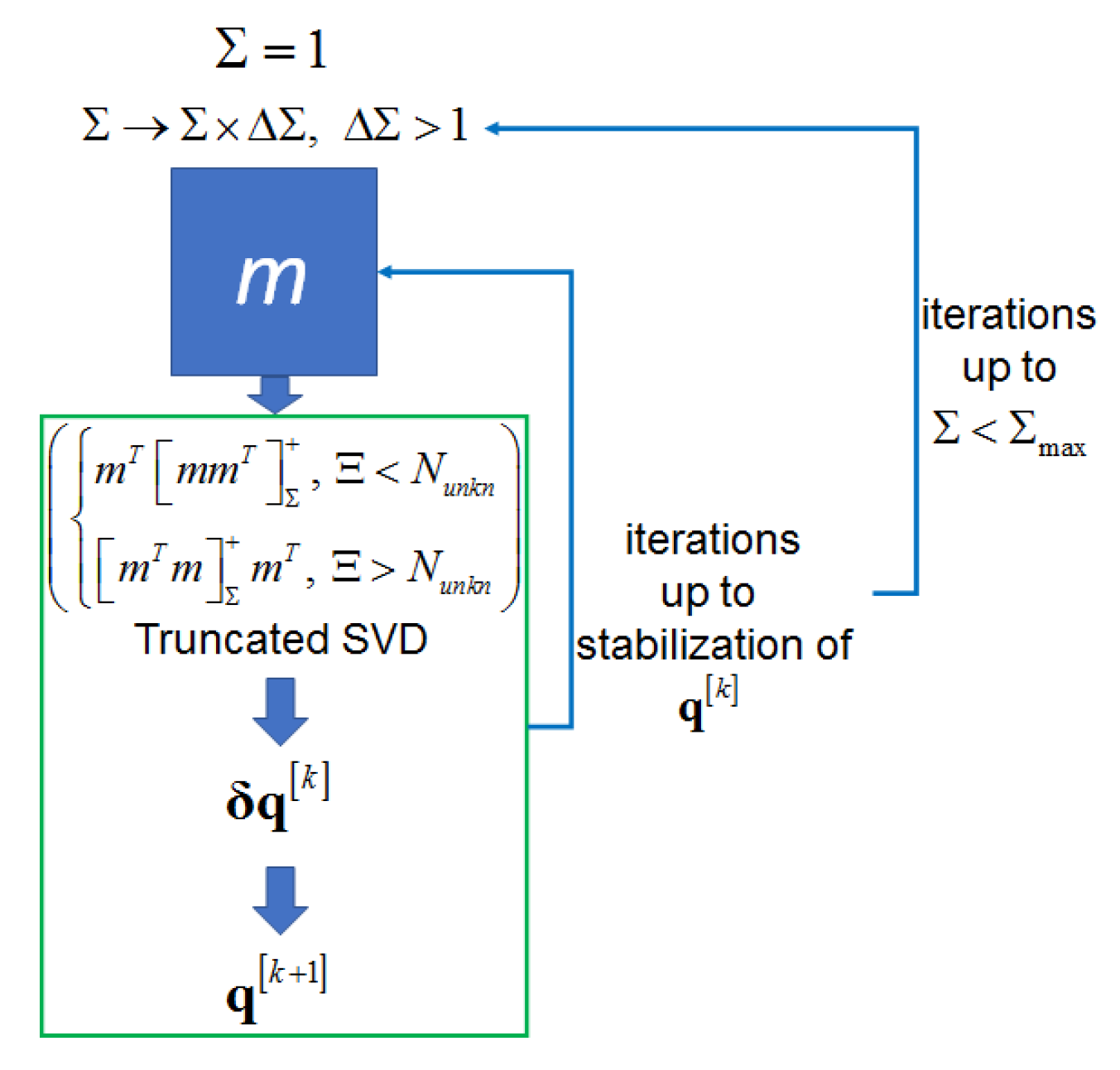
2.4. Parallelization Strategy

To solve the inverse problem by solving the ill-posed nonlinear (quasi-linear) operator Equation (11), we use Algorithm A1 from Appendix A. The computational scheme of the algorithm is shown in Figure 1, and it has three levels of nested loops:

• The outer loop increases the sensitivity operator’s matrix inversion regularization parameter $\Sigma$;
• The middle loop performs the Newton-type iterations up to the stabilization with the fixed $\Sigma$;
• The inner loop chooses the step parameter $\gamma$ in the Newton-type iterations to provide the monotonic decrease in the data misfit.

Figure 1. The principal scheme on the algorithm’s iterations (the outer and the middle loops), the inner loop is inside the green box. The most time-consuming part of the algorithm (more than $95\%$ of all computations) is constructing the sensitivity operator’s matrix m.

Figure 1. The principal scheme on the algorithm’s iterations (the outer and the middle loops), the inner loop is inside the green box. The most time-consuming part of the algorithm (more than $95\%$ of all computations) is constructing the sensitivity operator’s matrix m.

The iteration at the middle level constructs the sensitivity operator’s matrix $m=M_U[{\mathbf{q}}^{\left[k\right]},{\mathbf{q}}^{\left[k\right]}]$ according to (9) and builds the Newton-type update using Truncated SVD regularized inversion of m; the details can be found in Appendix A.

The most time-consuming part of the algorithm (more than $95\%$ of all computations, see

Table 1. Time results of sequential execution of the source identification algorithm with the considered scenario: $t_{IP}^{seq}$ is the total time of the inverse problem solution; $t_{SO}^{seq}$ is the total time of the sensitivity operator matrix construction; $p_{SO}^{seq}=t_{SO}^{seq}/t_{IP}^{seq}$ is the fraction of the time of inverse problem solution spent for sensitivity operator matrix construction.

Hardware	${\mathit{t}}_{\mathbf{IP}}^{\mathbf{seq}}$, sec	${\mathit{t}}_{\mathbf{SO}}^{\mathbf{seq}}$, sec	${\mathit{p}}_{\mathbf{SO}}^{\mathbf{seq}}$, %
Intel Xeon Phi 7290	461,257	442,233	95.9
Intel Xeon Gold 6248R	84,928	82,101	96.7

) is constructing the sensitivity operator’s matrix m, so this operation is the main target for parallel implementation. According to (9), the rows of m correspond to the ensemble of sensitivity functions

$$S^{\left[k\right]}=\{S[{\mathbf{q}}^{\left[k\right]},{\mathbf{q}}^{\left[k\right]};h^{\left(\xi \right)}],\xi =1,\dots ,\Xi \}.$$

(13)

In a naive way, we can evaluate the members of $S^{\left[k\right]}$ in parallel independently. This procedure can be optimized thanks to the similar nature of the ensemble members and reusing common aggregates of the sensitivity function calculation algorithms. To do this, we should consider the inner structure of the elements.

In the case of the source identification problem, the sensitivity function is evaluated according to ([12], Lemma 3.1). For the stationary sources ${\mathbf{r}}^{\left(2\right)},{\mathbf{r}}^{\left(1\right)}\in Q$, the sensitivity function is the temporal integral of the adjoint problem solution

$$S[{\mathbf{q}}^{\left(2\right)},{\mathbf{q}}^{\left[\right(1)};h]\left(\mathbf{x}\right)={\int }_0^T\mathsf{\Psi }(\mathbf{x},t)dt.$$

(14)

Here, $\mathsf{\Psi }(\mathbf{x},t)$ is the solution of the adjoint problem

$$\begin{array}{c}-\frac{\partial {\mathsf{\Psi }}_l}{\partial t}-\mathbf{u}·\nabla {\mathsf{\Psi }}_l-\nabla ·(\mathrm{diag}\left({\mu }_l\right)\nabla {\mathsf{\Psi }}_l)+{\left(\mathbf{W}\left(t,\mathbf{\phi }[{\mathbf{r}}^{\left(2\right)}],\mathbf{\phi }[{\mathbf{r}}^{\left(1\right)}]\right)\mathsf{\Psi }\right)}_l=h_l,\end{array}$$

$$\begin{array}{c}(\mathbf{x},t)\in {\mathsf{\Omega }}_T,\end{array}$$

(15)

$$\begin{array}{c}\mathbf{W}\left(t,\mathbf{a},\mathbf{b}\right)=\mathrm{diag}P(t,\mathbf{a})+{\rho }^{-1}\overline{\nabla }P{(t,\mathbf{a},\mathbf{b})}^T\rho \mathrm{diag}\mathbf{b}-{\rho }^{-1}\overline{\nabla }\Pi {(t,\mathbf{a},\mathbf{b})}^T\rho ,\end{array}$$

(16)

$$\begin{array}{c}\mathbf{n}·\left(\mathrm{diag}\left({\mu }_l\right)\nabla {\mathsf{\Psi }}_l+\mathbf{u}{\mathsf{\Psi }}_l\right)+\beta {\mathsf{\Psi }}_l=0,(\mathbf{x},t)\in {\Gamma }^{\left(out\right)}\subset \partial \mathsf{\Omega }\times [0,T],\end{array}$$

(17)

$$\begin{array}{c}{\mathsf{\Psi }}_l=0,(\mathbf{x},t)\in {\Gamma }^{\left(in\right)}\subset \partial \mathsf{\Omega }\times [0,T],\end{array}$$

(18)

$$\begin{array}{c}{\mathsf{\Psi }}_l=0,\mathbf{x}\in \mathsf{\Omega },t=T.\end{array}$$

(19)

In (16), the vector $\rho$ is the vector with elements ${\rho }_l$, and $P(t,\mathbf{a}),\Pi (t,\mathbf{a})$ are the vector-functions with the elements $P_l(t,\mathbf{a})$ and ${\Pi }_l(t,\mathbf{a})$, correspondingly for $l=1,\dots ,N_c$; and the symbol $\overline{\nabla }$ defines the divided difference operator ([55], p. 201) that maps vector-function $S:[0,T]\times {\mathbb{R}}^{N_c}\to {\mathbb{R}}^{N_c}$ to the vector function $\overline{\nabla }S:[0,T]\times {\mathbb{R}}^{N_c}\times {\mathbb{R}}^{N_c}\to {\mathbb{R}}^{N_c\times N_c}$, such that for any $t\in [0,T]$ and $\mathbf{\phi },\mathbf{\delta }\mathbf{\phi }\in {\mathbb{R}}^{N_c},$

$$S(t,\mathbf{\phi }+\delta \mathbf{\phi })-S(t,\mathbf{\phi })=\overline{\nabla }S(t,\mathbf{\phi }+\delta \mathbf{\phi },\mathbf{\phi })\delta \mathbf{\phi }.$$

We can see that the problem (15)–(19) is linear and all ensemble members share the same equation coefficients. In other words, we have to solve multiple linear problems that share the same numerical schemes coefficients and differ by right-hand sides only. Note that the ensemble of direct problem solutions would take the solution of nonlinear problems (1)–(4) with different right-hand sides. We evaluate the whole ensemble of the adjoint equation solutions backward in time, collecting $S^{\left[k\right]}$ according to (14).

Figure 2 illustrates our approaches to organizing the parallel evaluation of $S^{\left[k\right]}$ to obtain the rows of m:

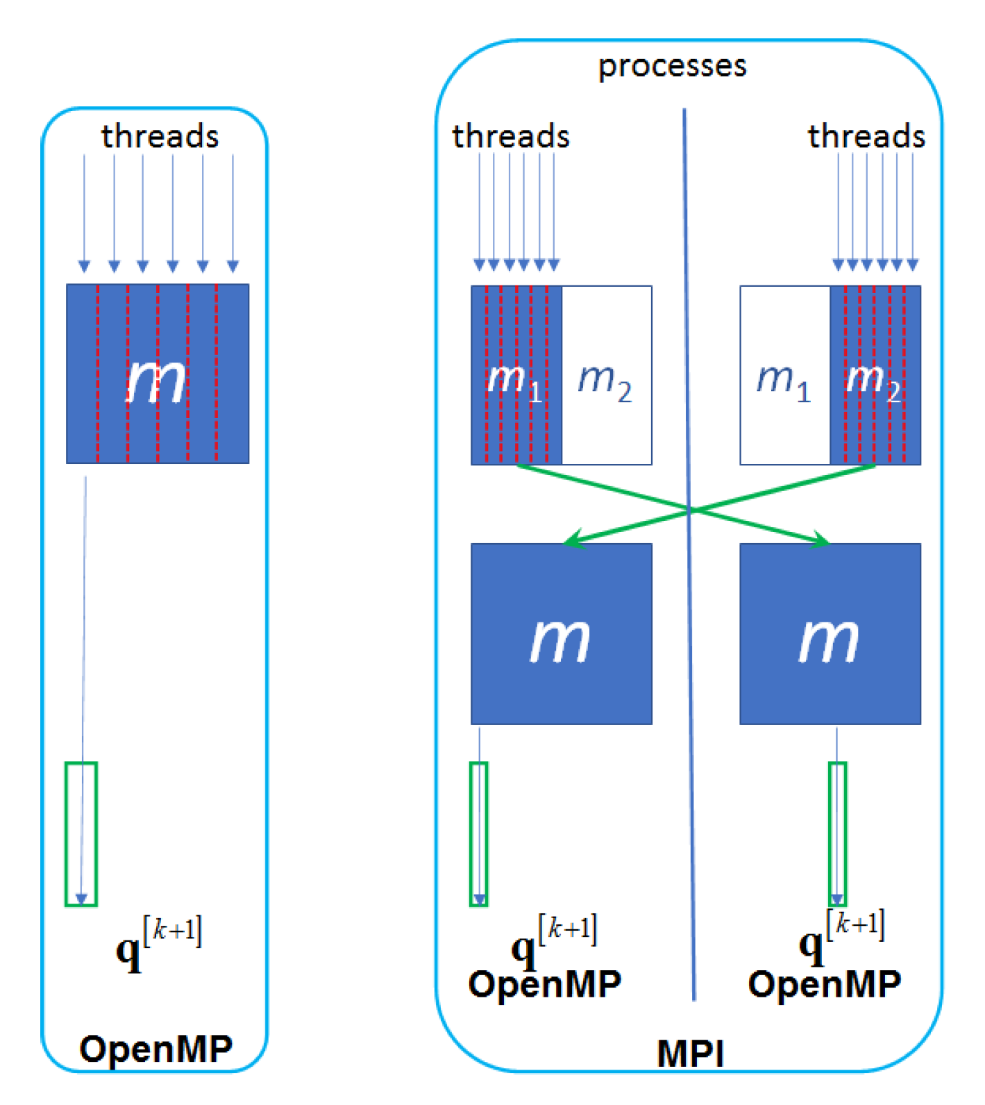
• For single-process execution, we use OpenMP parallelization technology [42]: each OpenMP thread constructs its set of the rows of m; after all rows are constructed and the whole m is built, one (the main) thread executes the sequential part of the iteration, i.e., inverts m and makes an update.
• For multiple-process execution, we use OpenMP for in-process parallelization and MPI for inter-process communications. Each MPI process executes the sequential part of the algorithm. In the parallel part, each process constructs its set of the rows of m; then the processes communicate with each other to form full m on each process.

Figure 2. Single-process (left) and multiple-process (right) parallelization schemes for the algorithm’s iterations. Parallelization is achieved by concurrent calculation of the rows of sensitivity operator matrix m. Green box corresponds to the green box in Figure 1 (sequential part of the iteration, i.e., inverting m and building update).

Figure 2. Single-process (left) and multiple-process (right) parallelization schemes for the algorithm’s iterations. Parallelization is achieved by concurrent calculation of the rows of sensitivity operator matrix m. Green box corresponds to the green box in Figure 1 (sequential part of the iteration, i.e., inverting m and building update).

Obviously, in this approach, the number of rows of sensitivity operator matrix determines the algorithm’s scalability, i.e., how many threads can concurrently execute the algorithm.

2.5. Experimental Setup

2.5.1. Inverse Modeling Scenario

For the objectives of the paper, we use the same “realistic” inverse modeling scenario as in [13], where the domain of the study contains the Baikal Natural Territory (Figure 3), which is recognized by UNESCO as a World Heritage Site [56]. The locations of the Roshydromet sites [57] are taken as the prototype of the measurement system in the scenario. We suppose that there are only $O_3$ concentration measurements ($L_{meas}=\{\#\left(O_3\right)\}$). Here, $\#\left(O_3\right)$ denotes the index of $O_3$ concentration in the state function $\mathbf{\phi }$.

The measurement sites in Figure 3 are divided into three groups with respect to the type of the “collected” measurements: concentration time series in a point, pointwise measurements in space and time, integrals over time domain in a point; the fourth type is a snapshot represented by the image of the simultaneous concentration distribution in the whole domain.

Time series are collected at 6 sites and are projected to 10 cosine Fourier basis elements resulting in 60 ($6\mathrm{sites}\times 10\mathrm{basis}\mathrm{elements}$) aggregates. Pointwise measurements are taken at 5 sites with 6-hour time intervals, thus producing 60 ($5\mathrm{sites}\times 12\mathrm{measurement}\mathrm{moments}$) aggregates. Integrals are collected at 5 sites producing 5 values. Snapshot is available on the third day of the scenario and is presented by 625 ($25\times 25$) projections to 2D cosine Fourier basis elements. Projection functions h corresponding to these types of measurements can be found in [13]. The total number of the measurement data aggregates $\Xi$ is equal to 750.

The value of $\Xi$ is an important parameter of the algorithm as the number of rows of the sensitivity operator’s matrix is equal to $\Xi$; therefore, according to Section 2.4, $\Xi$ determines the scalability of the parallel algorithm.

To obtain synthetic measurement data, we constructed a realistic “exact” emission source distribution $r^{(*)}$ as in [13] (Figure 4a). The initial guess is $r^{\left(0\right)}=0$, corresponding to $100\%$ relative error. A priory emission source is $\mathbf{f}=0$.

As the transformation model, we chose the atmospheric chemistry model (e.g., [58]) describing the photochemical $O_3-N{O}_x$ cycle:

$$\begin{array}{c}N{O}_2+h\nu \stackrel{y_1}{\to }NO+O{(}^{3}P),\end{array}$$

(20)

$$\begin{array}{c}O{(}^{3}P)+O_2\stackrel{y_2}{\to }{O}_3,\end{array}$$

(21)

$$\begin{array}{c}NO+O_3\stackrel{y_3}{\to }{O}_2+N{O}_2.\end{array}$$

(22)

The first reaction rate coefficient $y_1$ is time-dependent, and $y_2,y_3$ are constants:

$$\begin{array}{c}{y}_1\left(t\right)=\left\{\genfrac{}{}{0.0pt}{}{{10}^{-5}{e}^{sec\left(t\right)},\mathrm{at}\mathrm{day}\mathrm{time}}{{10}^{-40},\mathrm{at}\mathrm{night}\mathrm{time}}\right.,\end{array}$$

(23)

$$\begin{array}{c}sec\left(t\right)={\left(sin\left(\frac{\pi }{16}\left(\overline{t_h}-4\right)\right)\right)}^{0.2},\overline{t_h}=t_h-24int\left(\frac{t_h}{24}\right),t_h=\frac{t}{3600},\end{array}$$

(24)

$$\begin{array}{c}{y}_2=1.87\times {10}^{-14},y_3={10}^{-16},\end{array}$$

(25)

and $int\left(\frac{t_h}{24}\right)$ is the integer part of $\frac{t_h}{24}$. The concentration of $O_2$ is considered constant.

The initial concentration distributions ${\phi }_l^0$ are constant in the spatial domain $\mathsf{\Omega }$:

$$\begin{array}{c}\left[NO\right]\approx 0.002\frac{mg}{m^3},\left[N{O}_2\right]\approx 0.001\frac{mg}{m^3},\end{array}$$

(26)

$$\begin{array}{c}\left[O_2\right]\approx \mathrm{284,202}\frac{mg}{m^3},\left[O\right]=0\frac{mg}{m^3},\left[O_3\right]\approx 0.12\frac{mg}{m^3}.\end{array}$$

(27)

The boundary conditions are

$${\alpha }_l=\left\{\genfrac{}{}{0.0pt}{}{0,(\mathbf{x},t)\in {\Gamma }^{\left(out\right)}}{{\phi }_l^0,(\mathbf{x},t)\in {\Gamma }^{\left(in\right)}}\right.,{\beta }_l=0,$$

(28)

where ${\phi }_l^0$ is the constant value of the corresponding initial conditions. The values ${\phi }_l^0$ denote the background concentrations of the considered substances.

The results of the COSMO model [59] simulations for the period 2019-07-23 T12:00:00 to 2019-08-03 T12:00:00 are used as the 2D wind speed vector field $\mathbf{u}$ at the surface level. The diffusion coefficient $\mu =1000$ m${}^2$/s is chosen as a constant one.

The “exact” concentration distribution ${\phi }^{(*)}$ is generated by solving the direct problem with $r^{(*)}$. The synthetic measurement data, which are provided to the source reconstruction algorithm, is obtained from the $O_3$ elements of ${\phi }^{(*)}$. The result of the source reconstruction is presented in Figure 4b.

The calculations are carried out on a grid of $N_x=57$ by $N_y=60$ points in space, $N_t=$ 18,801 points in time, and $N_c=5$ chemicals. The time step $\Delta t=54$ seconds is demanded for the correct simulation of chemical transformations (20)–(25). Thus, the dimension of the state function is $N_t\times N_x\times N_y\times N_c=$ 321,497,100 elements. The dimension of the unknowns that have to be estimated by given $\Xi =750$ aggregated values is $N_x\times N_y=3420$.

Sequential execution of the source identification algorithm with this scenario takes about 5 days on an Intel Xeon Phi 7290 1.50 GHz 96 GB RAM node and about 1 day on an Intel Xeon Gold 6248R 3.00 GHz 384 GB RAM (Table 1).

2.5.2. Hardware Configuration

The experiments with HPC were carried out in the Siberian Supercomputer Center on the NKS-30T Hybrid cluster. The following configurations are used:

• Single node with Intel Xeon Phi 7290 (1 CPU × 72 cores × 4 threads, 1.50 GHz, 96 GB RAM). Total number of cores is 72, and the maximum number of processing threads is 288.
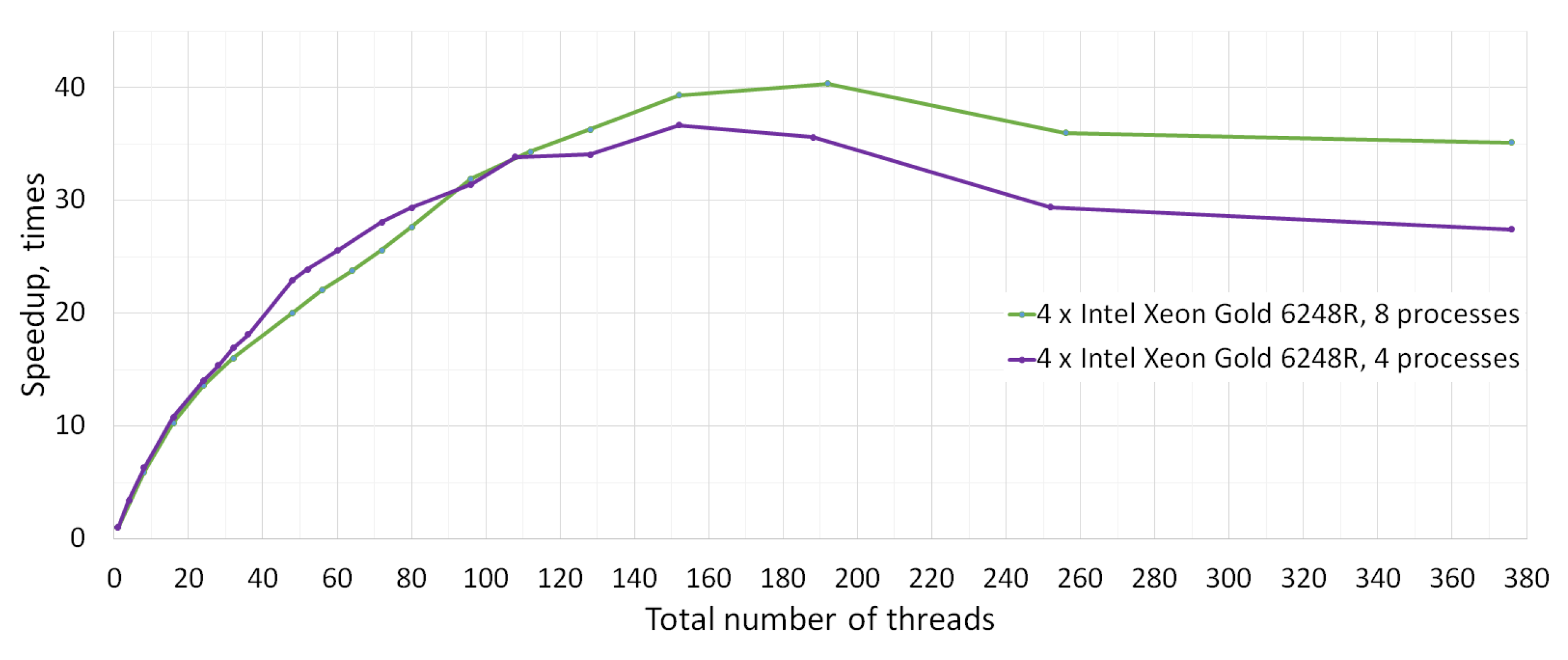
• Total of 1, 2, 3, and 4 nodes with Intel Xeon Gold 6248R (2 CPU × 24 cores × 2 threads, 3.00 GHz, 384 GB RAM) connected with Cluster Interconnect Omni-Path 100 Gbps. Total number of cores/threads is 48/96, 96/192, 144/288, and 192/384, correspondingly. For each number of nodes, we tested:

  −

  “Single process per node” execution,

  −

  “Two processes per node” execution with each process running on separate CPU.

  In multiple-process execution, all the processes launch an equal number of OpenMP threads, so the total number of threads is a multiple of the number of processes.

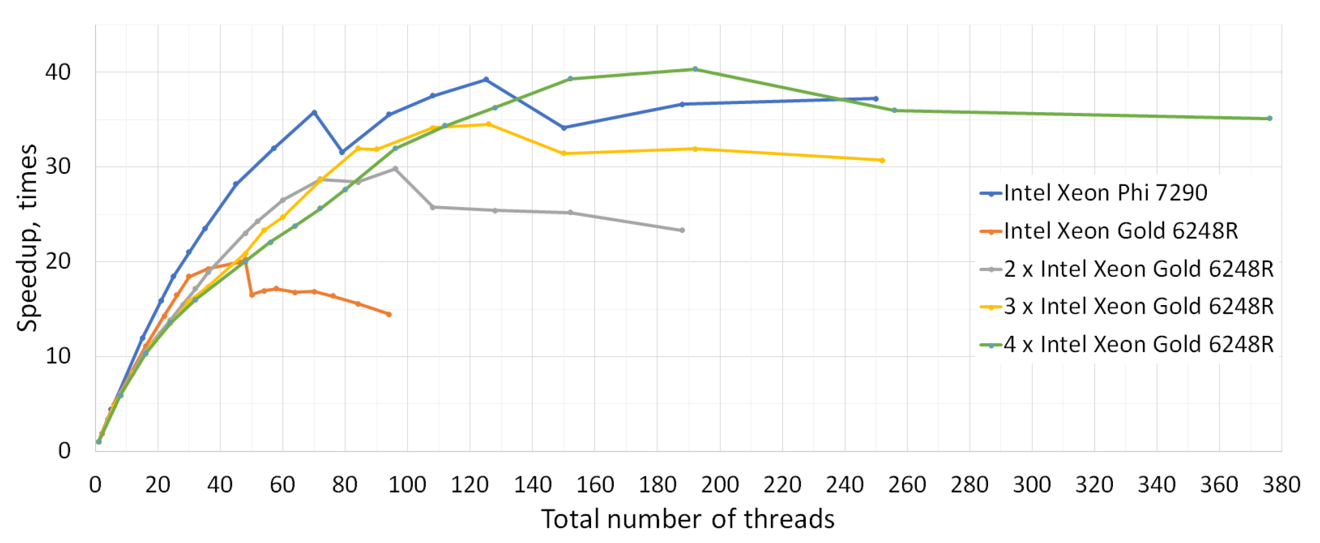
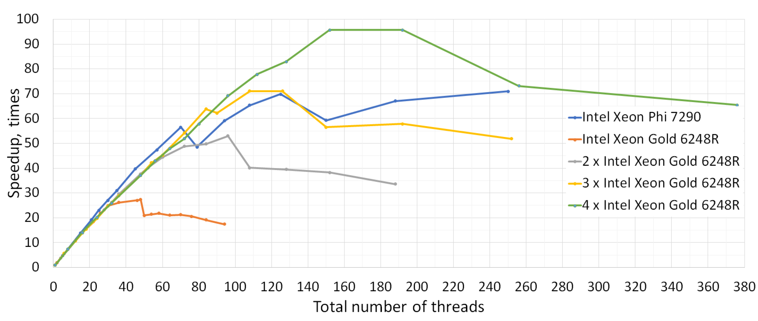
The main principle for choosing the number of threads to test the algorithm is the minimization of the total idle threads. As, in our scenario, the value of $\Xi$ (the number of rows of sensitivity operator matrix m and, therefore, the number of independent “pieces of work” for constructing m) is 750, it makes sense to test the algorithm against, say, 375 threads (each thread constructs 2 rows, no idle) or 250 threads (each thread constructs 3 rows, no idle), but not against 300 threads (150 threads per 2 rows plus 150 per 3 rows; execution time is “3 rows”, and the total idle is ($3\times 150-2\times 150$) = “150 rows”).

3. Results

The results of the computational experiments are demonstrated in Table 2 and Figure 5, Figure 6 and Figure 7:

• Table 2 summarizes various time characteristics of parallel execution for different hardware configurations.
• Figure 5 and Figure 6 show the speedup achieved with different hardware configurations and the number of executing threads for inverse problem solution and for sensitivity operator matrix construction, correspondingly.
• Figure 7 compares the performance of two approaches to parallel execution: “single process per node” and “single process per CPU”.

Figure 5. Speedup of inverse problem solution on different hardware configurations. The best values are achieved with the numbers of threads equal to the number of processor cores (for Intel Xeon Phi node, twice the number of cores).

Figure 5. Speedup of inverse problem solution on different hardware configurations. The best values are achieved with the numbers of threads equal to the number of processor cores (for Intel Xeon Phi node, twice the number of cores).

Figure 6. Speedup of sensitivity operator matrix construction on different hardware configurations. The best values are achieved with the numbers of threads equal to the number of processor cores (for Intel Xeon Phi node, triple the number of cores).

Figure 6. Speedup of sensitivity operator matrix construction on different hardware configurations. The best values are achieved with the numbers of threads equal to the number of processor cores (for Intel Xeon Phi node, triple the number of cores).

Figure 7. Speedup of four-node executions of the inverse problem solution with four (one per two-CPU node) and eight (two per node with CPU affinity) MPI processes. For a large number of threads, the option with CPU affinity provides better results despite the additional costs of duplicating calculations.

Figure 7. Speedup of four-node executions of the inverse problem solution with four (one per two-CPU node) and eight (two per node with CPU affinity) MPI processes. For a large number of threads, the option with CPU affinity provides better results despite the additional costs of duplicating calculations.

Table 2. Time results of the inverse problem solution on different hardware configurations: $t_{IP}^{seq}$ is the time of the sequential inverse problem solution; $t_{IP}^{par}$ is the best time of the parallel inverse problem solution; $s_{IP}=t_{IP}^{seq}/t_{IP}^{par}$ is the best speedup; $N_{IP}$ is the total number of threads with which the best speedup was achieved; $n_{IP}$ is the number of threads per node with which the best speedup was achieved; $e_{IP}=s_{IP}/N_{IP}$ is the parallelization efficiency for best speedup; $t_{SO}^{par}$ is the time of sensitivity operator’s matrix construction with $N_{IP}$ threads; $p_{SO}^{par}=t_{SO}^{par}/t_{IP}^{par}$ is the fraction of time of parallel inverse problem solution spent for the sensitivity operator’s matrix construction.

Hardware	${\mathit{t}}_{\mathbf{IP}}^{\mathbf{seq}}$, sec	${\mathit{t}}_{\mathbf{IP}}^{\mathbf{par}}$, sec	${\mathit{s}}_{\mathbf{IP}}$	${\mathit{N}}_{\mathbf{IP}}$	${\mathit{n}}_{\mathbf{IP}}$	${\mathit{e}}_{\mathbf{IP}}$, %	${\mathit{t}}_{\mathbf{SO}}^{\mathbf{par}}$, sec	${\mathit{p}}_{\mathbf{SO}}^{\mathbf{par}}$, %
1 × Intel Xeon Phi 7290	461,257	11,758	39.23	125	125	31.4	6336	53.9
1 × Intel Xeon Gold 6248R	84,928	4195	20.25	48	48	42.2	3003	71.6
2 × Intel Xeon Gold 6248R	84,928	2847	29.83	96	48	31.1	1551	54.5
3 × Intel Xeon Gold 6248R	84,928	2460	34.52	126	42	27.4	1155	47.0
4 × Intel Xeon Gold 6248R	84,928	2105	40.35	192	48	21.0	858	40.8

Table 2. Time results of the inverse problem solution on different hardware configurations: $t_{IP}^{seq}$ is the time of the sequential inverse problem solution; $t_{IP}^{par}$ is the best time of the parallel inverse problem solution; $s_{IP}=t_{IP}^{seq}/t_{IP}^{par}$ is the best speedup; $N_{IP}$ is the total number of threads with which the best speedup was achieved; $n_{IP}$ is the number of threads per node with which the best speedup was achieved; $e_{IP}=s_{IP}/N_{IP}$ is the parallelization efficiency for best speedup; $t_{SO}^{par}$ is the time of sensitivity operator’s matrix construction with $N_{IP}$ threads; $p_{SO}^{par}=t_{SO}^{par}/t_{IP}^{par}$ is the fraction of time of parallel inverse problem solution spent for the sensitivity operator’s matrix construction.

Hardware	${\mathit{t}}_{\mathbf{IP}}^{\mathbf{seq}}$, sec	${\mathit{t}}_{\mathbf{IP}}^{\mathbf{par}}$, sec	${\mathit{s}}_{\mathbf{IP}}$	${\mathit{N}}_{\mathbf{IP}}$	${\mathit{n}}_{\mathbf{IP}}$	${\mathit{e}}_{\mathbf{IP}}$, %	${\mathit{t}}_{\mathbf{SO}}^{\mathbf{par}}$, sec	${\mathit{p}}_{\mathbf{SO}}^{\mathbf{par}}$, %
1 × Intel Xeon Phi 7290	461,257	11,758	39.23	125	125	31.4	6336	53.9
1 × Intel Xeon Gold 6248R	84,928	4195	20.25	48	48	42.2	3003	71.6
2 × Intel Xeon Gold 6248R	84,928	2847	29.83	96	48	31.1	1551	54.5
3 × Intel Xeon Gold 6248R	84,928	2460	34.52	126	42	27.4	1155	47.0
4 × Intel Xeon Gold 6248R	84,928	2105	40.35	192	48	21.0	858	40.8

4. Discussion

As one can see from Figure 5, the speedup of the inverse problem solution grows until the number of threads becomes equal to the number of processor cores (for Intel Xeon Phi node, twice the number of cores), i.e., involving the second (for Intel Xeon Phi node, the third and the forth) threads of the cores results in no further speedup. With this limitation, the parallel code shows satisfactory efficiency of $20\%$ on 192 threads (40× speedup). Such a big speedup value may look contradicting to Table 1, which states that the “sequential” part of the algorithm takes 3–5% of total calculations (and, therefore, the “ideal” speedup is limited by the values of 20–30), but can be explained by the presence of some in-process parallelization inside the “sequential” part.

Figure 6 focuses on the time results of the sensitivity operator matrix construction and allows us to look at parallelization effects in isolation. The operation shows parallelization efficiency of $63\%$ for 152 threads (95× speedup). In other words, the additional cost of 152-thread parallelism (scheduling, tasking, and synchronization by MPI and OpenMP plus concurrent memory access conflicts resolution by hardware) is only about $37\%$ of computation time, which can be considered good efficiency.

Another interesting point is that a single Intel Xeon Phi node provides a speedup comparable to several (3 for the sensitivity operator matrix construction and 4 for the inverse problem solution) Intel Xeon Gold nodes. This effect is more significant for the inverse problem solution due to the in-process parallelization in the “sequential” part mentioned above; as the execution of the “sequential” part is duplicated by each processing node, the number of threads executing the “sequential” part is greater for single process execution (all the processing threads) than for multiple process execution (some fraction of all the processing threads). Furthermore, the speedup that the single Intel Xeon Phi provides for the sensitivity operator matrix construction grows until the hardware thread exhaustion (the best value is achieved with 250 threads). These facts, together with the lower cost of Intel Xeon Phi, makes it an attractive facility for HPC.

Finally, it turned out that, starting with the number of threads equal to half of the number of cores, launching two MPI processes with CPU affinity on Intel Xeon Gold node rather than one, provides better performance, despite the redundant calculations introduced by the duplication of the “sequential” parts of the algorithm in each process. Figure 7 shows this for a four-node execution, and a similar picture is observed for other setups. This can be explained by the nature of non-uniform memory access (NUMA) architecture, which is used in the vast majority of multiprocessors (such as Intel Xeon Gold nodes):

• The OpenMP threads 1–24 are executed by one CPU of Intel Xeon Gold and the threads 25–48, by another;
• The memory allocated by a thread is taken from the local memory of the CPU running the thread;
• CPU accesses its own local memory faster than non-local memory.

As a result, if a process runs 24 OpenMP threads or less, all its threads are executed by a single CPU and allocate and access only local memory. However, if a process runs 25 OpenMP threads or more, some threads executed by one CPU access other CPU’s local memory, which is less effective. For our code, the overhead of accessing non-local memory is greater than the one of duplicating the “sequential” part of calculations.

Table 2 shows that the use of HPC allows us to shorten the inverse problem solution drastically: for Intel Xeon Phi, from 5 days to less than 4 h, and for 4 Intel Xeon Gold nodes, from 1 day to 35 min.

The fraction of time spent for the “parallel” part of the program decreased from 95% to 40%; therefore, involving additional threads in processing will not result in significant acceleration with our modeling scenario, which can be considered one of the limitations of the work. Furthermore, a limitation is relatively high memory consumption compared to the gradient-based algorithms due to solving multiple adjoint problems instead of a single one. This limitation is common for the ensemble-based algorithms, which makes it difficult to use our approach directly in realistic cases on GPU-like architectures.

5. Conclusions

Large-scale inverse problems demand both efficient algorithms and the implementation of the modern computational infrastructure. In the paper, we presented the evaluation results of MPI implementation of the source identification algorithm based on the sensitivity operators and adjoint ensembles in the inverse modeling scenario for Lake Baikal region, which allows using large HPC systems.

The implementation drastically shortens modeling time in the scenario from days to tens of minutes and provides satisfactory scalability up to 200 executing threads. It is shown that launching two MPI processes on a two-processor node with CPU affinity provides better performance than the “one process per node” setup despite some redundancy of calculation. The achieved results contribute to the wider application of inverse modeling in large-scale studies. As a possible future work, we consider:

• Increasing overall efficiency of IMDAF code at micro (loop vectorization, memory access optimization) and macro (using highly optimized libraries, decreasing memory footprint) levels;
• Introducing parallelism into the “sequential” part of the program;
• Analyzing and mitigating the factors limiting the speedup of sensitivity operator matrix construction;
• Testing more realistic and time-consuming models and scenarios (including more complicated chemistry model and 3D space modeling);
• Using the software in the thematic services for air quality studies.

References

1. Brunet, G. Seamless Prediction of the Earth System: From Minutes to Months; World Meteorological Organization: Geneva, Switzerland, 2015. [Google Scholar]
2. World Meteorological Organization. Guide to Instruments and Methods of Observation; Volume I –Measurement of Meteorological Variables, Chapter Measurement of Atmospheric Composition; WMO: Geneva, Switzerland, 2018; pp. 506–541. [Google Scholar]
3. Sokhi, R.S.; Moussiopoulos, N.; Baklanov, A.; Bartzis, J.; Coll, I.; Finardi, S.; Friedrich, R.; Geels, C.; Grönholm, T.; Halenka, T.; et al. Advances in air quality research—current and emerging challenges. Atmos. Chem. Phys. 2022, 22, 4615–4703. [Google Scholar] [CrossRef]
4. Bocquet, M.; Elbern, H.; Eskes, H.; Hirtl, M.; Žabkar, R.; Carmichael, G.R.; Flemming, J.; Inness, A.; Pagowski, M.; Camaño, J.L.P.; et al. Data assimilation in atmospheric chemistry models: Current status and future prospects for coupled chemistry meteorology models. Atmos. Chem. Phys. Discuss. 2014, 14, 32233–32323. [Google Scholar] [CrossRef] [Green Version]
5. Carrassi, A.; Bocquet, M.; Bertino, L.; Evensen, G. Data assimilation in the geosciences: An overview of methods, issues, and perspectives. Wiley Interdiscip. Rev. Clim. Chang. 2018, 9, e535. [Google Scholar] [CrossRef] [Green Version]
6. Elbern, H.; Strunk, A.; Schmidt, H.; Talagrand, O. Emission rate and chemical state estimation by 4-dimensional variational inversion. Atmos. Chem. Phys. Discuss. 2007, 7, 1725–1783. [Google Scholar] [CrossRef] [Green Version]
7. Holnicki, P.; Nahorski, Z. Emission Data Uncertainty in Urban Air Quality Modeling—Case Study. Environ. Model. Assess. 2015, 20, 583–597. [Google Scholar] [CrossRef] [Green Version]
8. Markakis, K.; Valari, M.; Perrussel, O.; Sanchez, O.; Honore, C. Climate-forced air-quality modeling at the urban scale: Sensitivity to model resolution, emissions and meteorology. Atmos. Chem. Phys. 2015, 15, 7703–7723. [Google Scholar] [CrossRef] [Green Version]
9. Zlatev, Z. Computer Treatment of Large Air Pollution Models; Springer: Dordrecht, The Netherlands, 1995. [Google Scholar] [CrossRef]
10. Baklanov, A.; Alexander, M.; Sokhi, R. (Eds.) Integrated Systems of Meso—Meteorological and Chemical Transport Models; Springer: Berlin/Heidelberg, Germany, 2011. [Google Scholar] [CrossRef]
11. Cullen, M.; Freitag, M.A.; Kindermann, S.; Scheichl, R. (Eds.) Large Scale Inverse Problems; DE GRUYTER: Berlin, Germany; Boston, MA, USA, 2013. [Google Scholar] [CrossRef] [Green Version]
12. Penenko, A. Convergence analysis of the adjoint ensemble method in inverse source problems for advection-diffusion-reaction models with image-type measurements. Inverse Probl. Imaging 2020, 14, 757–782. [Google Scholar] [CrossRef]
13. Penenko, A.; Penenko, V.; Tsvetova, E.; Gochakov, A.; Pyanova, E.; Konopleva, V. Sensitivity Operator Framework for Analyzing Heterogeneous Air Quality Monitoring Systems. Atmosphere 2021, 12, 1697. [Google Scholar] [CrossRef]
14. Penenko, A.; Zubairova, U.; Mukatova, Z.; Nikolaev, S. Numerical algorithm for morphogen synthesis region identification with indirect image-type measurement data. J. Bioinform. Comput. Biol. 2019, 17, 1940002-1–1940002-18. [Google Scholar] [CrossRef]
15. Marchuk, G.I. Formulation of some converse problems. Sov. Math. Dokl. 1964, 5, 675–678. [Google Scholar]
16. Penenko, V. Methods for Numerical Simulation of Atmospheric Processes; Hydrometeoizdat: Leningrad, Russia, 1981. (In Russian) [Google Scholar]
17. Murio, D.A. The Mollification Method and the Numerical Solution of Ill-Posed Problems; John Wiley & Sons, Inc.: New York, NY, USA, 1993. [Google Scholar] [CrossRef]
18. Dimet, F.X.L.; Souopgui, I.; Titaud, O.; Shutyaev, V.; Hussaini, M.Y. Toward the assimilation of images. Nonlinear Process. Geophys. 2015, 22, 15–32. [Google Scholar] [CrossRef] [Green Version]
19. Anderson, J.L.; Collins, N. Scalable Implementations of Ensemble Filter Algorithms for Data Assimilation. J. Atmos. Ocean. Technol. 2007, 24, 1452–1463. [Google Scholar] [CrossRef]
20. Li, X.; Lu, W. Particle network EnKF for large-scale data assimilation. Front. Phys. 2022, 10, 850. [Google Scholar] [CrossRef]
21. Ghorbanidehno, H.; Kokkinaki, A.; Lee, J.; Darve, E. Recent developments in fast and scalable inverse modeling and data assimilation methods in hydrology. J. Hydrol. 2020, 591, 125266. [Google Scholar] [CrossRef]
22. Todaro, V.; D’Oria, M.; Tanda, M.G.; Gómez-Hernández, J.J. genES-MDA: A generic open-source software package to solve inverse problems via the Ensemble Smoother with Multiple Data Assimilation. Comput. Geosci. 2022, 167, 105210. [Google Scholar] [CrossRef]
23. Anderson, J.; Hoar, T.; Raeder, K.; Liu, H.; Collins, N.; Torn, R.; Avellano, A. The Data Assimilation Research Testbed: A Community Facility. Bull. Am. Meteorol. Soc. 2009, 90, 1283–1296. [Google Scholar] [CrossRef] [Green Version]
24. Nerger, L.; Hiller, W. Software for ensemble-based data assimilation systems—Implementation strategies and scalability. Comput. Geosci. 2013, 55, 110–118. [Google Scholar] [CrossRef]
25. Nerger, L.; Tang, Q.; Mu, L. Efficient ensemble data assimilation for coupled models with the Parallel Data Assimilation Framework: Example of AWI-CM (AWI-CM-PDAF 1.0). Geosci. Model Dev. 2020, 13, 4305–4321. [Google Scholar] [CrossRef]
26. Browne, P.; Wilson, S. A simple method for integrating a complex model into an ensemble data assimilation system using MPI. Environ. Model. Softw. 2015, 68, 122–128. [Google Scholar] [CrossRef] [Green Version]
27. Huang, D.Z.; Huang, J.; Reich, S.; Stuart, A.M. Efficient derivative-free Bayesian inference for large-scale inverse problems. Inverse Probl. 2022, 38, 125006. [Google Scholar] [CrossRef]
28. Cho, T.; Chung, J.; Miller, S.M.; Saibaba, A.K. Computationally efficient methods for large-scale atmospheric inverse modeling. Geosci. Model Dev. 2022, 15, 5547–5565. [Google Scholar] [CrossRef]
29. Pandey, S.; Houweling, S.; Segers, A. Order of magnitude wall time improvement of variational methane inversions by physical parallelization: A demonstration using TM5-4DVAR. Geosci. Model Dev. 2022, 15, 4555–4567. [Google Scholar] [CrossRef]
30. D’Amore, L.; Constantinescu, E.; Carracciuolo, L. A Scalable Space-Time Domain Decomposition Approach for Solving Large Scale Nonlinear Regularized Inverse Ill Posed Problems in 4D Variational Data Assimilation. J. Sci. Comput. 2022, 91, 59. [Google Scholar] [CrossRef]
31. Hamill, T.M.; Snyder, C. A Hybrid Ensemble Kalman Filter–3D Variational Analysis Scheme. Mon. Weather. Rev. 2000, 128, 2905–2919. [Google Scholar] [CrossRef]
32. Pisso, I.; Sollum, E.; Grythe, H.; Kristiansen, N.I.; Cassiani, M.; Eckhardt, S.; Arnold, D.; Morton, D.; Thompson, R.L.; Zwaaftink, C.D.G.; et al. The Lagrangian particle dispersion model FLEXPART version 10.4. Geosci. Model Dev. 2019, 12, 4955–4997. [Google Scholar] [CrossRef] [Green Version]
33. Bergamaschi, P.; Segers, A.; Brunner, D.; Haussaire, J.M.; Henne, S.; Ramonet, M.; Arnold, T.; Biermann, T.; Chen, H.; Conil, S.; et al. High-resolution inverse modelling of European CH4 emissions using the novel FLEXPART-COSMO TM5 4DVAR inverse modelling system. Atmos. Chem. Phys. 2022, 22, 13243–13268. [Google Scholar] [CrossRef]
34. Leeuwen, P.J.; Kunsch, H.R.; Nerger, L.; Potthast, R.; Reich, S. Particle filters for high-dimensional geoscience applications: A review. Q. J. R. Meteorol. Soc. 2019, 145, 2335–2365. [Google Scholar] [CrossRef] [PubMed]
35. Penny, S.G.; Smith, T.A.; Chen, T.C.; Platt, J.A.; Lin, H.Y.; Goodliff, M.; Abarbanel, H.D.I. Integrating Recurrent Neural Networks With Data Assimilation for Scalable Data-Driven State Estimation. J. Adv. Model. Earth Syst. 2022, 14, e2021MS002843. [Google Scholar] [CrossRef]
36. Biondi, E.; Barnier, G.; Clapp, R.G.; Picetti, F.; Farris, S. An object-oriented optimization framework for large-scale inverse problems. Comput. Geosci. 2021, 154, 104790. [Google Scholar] [CrossRef]
37. Villa, U.; Petra, N.; Ghattas, O. hIPPYlib An Extensible Software Framework for Large-Scale Inverse Problems Governed by PDEs: Part I: Deterministic Inversion and Linearized Bayesian Inference. ACM Trans. Math. Softw. 2021, 47, 1–34. [Google Scholar] [CrossRef]
38. Issartel, J.P. Emergence of a tracer source from air concentration measurements, a new strategy for linear assimilation. Atmos. Chem. Phys. 2005, 5, 249–273. [Google Scholar] [CrossRef] [Green Version]
39. Mamonov, A.V.; Tsai, Y.H.R. Point source identification in nonlinear advection-diffusion-reaction systems. Inverse Probl. 2013, 29, 035009. [Google Scholar] [CrossRef] [Green Version]
40. Bieringer, P.E.; Young, G.S.; Rodriguez, L.M.; Annunzio, A.J.; Vandenberghe, F.; Haupt, S.E. Paradigms and commonalities in atmospheric source term estimation methods. Atmos. Environ. 2017, 156, 102–112. [Google Scholar] [CrossRef] [Green Version]
41. Panasenko, E.A.; Starchenko, A.V. Determination of urban district atmospheric air pollution in accordance with observational data. Atmos. Ocean. Opt. 2009, 22, 186–191. [Google Scholar] [CrossRef]
42. Penenko, A.; Gochakov, A. Parallel speedup analysis of an adjoint ensemble-based source identification algorithm. J. Phys. Conf. Ser. 2021, 1715, 012072-1–012072-6. [Google Scholar] [CrossRef]
43. Johnson, S.G. The NLopt Nonlinear-Optimization Package. Available online: http://github.com/stevengj/nlopt (accessed on 31 October 2022).
44. Boussaid, I.; Lepagnot, J.; Siarry, P. A survey on optimization metaheuristics. Inf. Sci. 2013, 237, 82–117. [Google Scholar] [CrossRef]
45. Biscani, F.; Izzo, D. A parallel global multiobjective framework for optimization: Pagmo. J. Open Source Softw. 2020, 5, 2338. [Google Scholar] [CrossRef]
46. Penenko, A.V.; Konopleva, V.S.; Penenko, V.V. Inverse modeling of atmospheric chemistry with a differential evolution solver: Inverse problem and Data assimilation. IOP Conf. Ser. Earth Environ. Sci. 2022, 1023, 012015. [Google Scholar] [CrossRef]
47. Penenko, A.; Konopleva, V.; Bobrovskikh, A. Numerical Comparison of the Adjoint Problem-based and Derivative-free Algorithms on the Coefficient Identification Problem for a Production-Loss Model. In Proceedings of the 2021 17th International Asian School-Seminar Optimization Problems of Complex Systems (OPCS), Novosibirsk, Russia, 13–17 September 2021. [Google Scholar] [CrossRef]
48. Galassi, M. GNU Scientific Library Reference Manual-Third Edition; Network Theory Ltd., 2009; ISBN 0954612078. Available online: https://dl.acm.org/doi/10.5555/1538674 (accessed on 31 October 2022).
49. Penenko, A.; Nikolaev, S.; Golushko, S.; Romashenko, A.; Kirilova, I. Numerical Algorithms for Diffusion Coefficient Identification in Problems of Tissue Engineering. Math. Biol. Bioinform. 2016, 11, 426–444. [Google Scholar] [CrossRef] [Green Version]
50. Penenko, A. A Newton-Kantorovich Method in Inverse Source Problems for Production-Destruction Models with Time Series-Type Measurement Data. Numer. Anal. Appl. 2019, 12, 51–69. [Google Scholar] [CrossRef]
51. Heimbach, P.; Hill, C.; Giering, R. An efficient exact adjoint of the parallel MIT General Circulation Model, generated via automatic differentiation. Future Gener. Comput. Syst. 2005, 21, 1356–1371. [Google Scholar] [CrossRef]
52. Vlasenko, A.; Kohl, A.; Stammer, D. The efficiency of geophysical adjoint codes generated by automatic differentiation tools. Comput. Phys. Commun. 2016, 199, 22–28. [Google Scholar] [CrossRef] [Green Version]
53. Naumann, U. Adjoint Code Design Patterns. ACM Trans. Math. Softw. 2019, 45, 1–32. [Google Scholar] [CrossRef] [Green Version]
54. Rew, R.; Davis, G. NetCDF: An interface for scientific data access. IEEE Comput. Graph. Appl. 1990, 10, 76–82. [Google Scholar] [CrossRef]
55. Ortega, J.M.; Rheinboldt, W.C. Iterative Solution of Nonlinear Equations in Several Variables; Academic Press: New York, NY, USA, 1970. [Google Scholar]
56. UNESCO. Lake Baikal. Available online: https://whc.unesco.org/en/list/754/ (accessed on 1 December 2021).
57. Roshydromet. Unified Information System for Monitoring Atmospheric Air Pollution. Available online: http://www.feerc.ru/uisem/portal/ad/irkutsk (accessed on 1 November 2021). (In Russian).
58. Hundsdorfer, W.; Verwer, J.G. Numerical Solution of Time-Dependent Advection-Diffusion-Reaction Equations; Springer Series in Computational Mathematics; Springer: Berlin/Heidelberg, Germany, 2013. [Google Scholar]
59. Baldauf, M.; Seifert, A.; Forstner, J.; Majewski, D.; Raschendorfer, M.; Reinhardt, T. Operational Convective-Scale Numerical Weather Prediction with the COSMO Model: Description and Sensitivities. Mon. Weather. Rev. 2011, 139, 3887–3905. [Google Scholar] [CrossRef]
60. Cheverda, V.A.; Kostin, V.I. R-pseudoinverses for compact operators in Hilbert spaces: Existence and stability. J. Inverse Ill-Posed Probl. 1995, 3, 131–148. [Google Scholar] [CrossRef]
61. Guennebaud, G.; Jacob, B. Eigen v3. 2010. Available online: http://eigen.tuxfamily.org (accessed on 31 October 2022).
Figure 3. Geographical domain and the monitoring site locations collecting time series (red crosses), pointwise measurements (blue circles) and integral measurements (magenta triangles) of ozone ( O 3 ) concentrations.
Mathematics 10 04522 g003
Figure 4. “Exact” configuration of emission sources (a) and reconstructed sources (b) of N O from [13].
Mathematics 10 04522 g004