Article

Why Is Aedes aegypti Moving South in South America?

by
Lucas Ernesto Alonso
1,
Victoria Romeo Aznar
2 and
Hernán Gustavo Solari
3,*
1
Instituto de Investigaciones en Energía No Convencional (INENCO), UNSa-CONICET, Salta 4400, Argentina
2
Instituto de Ecología, Genética y Evolución de Buenos Aires (IEGEBA), UBA-CONICET and Departamento de Ecología, Genética y Evolución, FCEN-UBA, Ciudad Autónoma de Buenos Aires 1428, Argentina
3
Inistituto de Física de Buenos Aires (IFIBA), UBA-CONICET and Departmento de Física, FCEN-UBA, Ciudad Autónoma de Buenos Aires 1428, Argentina
*
Author to whom correspondence should be addressed.
Mathematics 2022, 10(23), 4510; https://doi.org/10.3390/math10234510
Submission received: 22 October 2022 / Revised: 15 November 2022 / Accepted: 22 November 2022 / Published: 29 November 2022

Abstract

:
Colonies of Aedes aegypti have been reported at increasingly southern locations. Is this feature a manifestation of climate change or the result of the mosquito’s adaptation? Answering the question requires the testing and comparison of results produced under different, competing, hypotheses. We address the problem using “AedesBA”, a detailed model of the mosquito Aedes aegypti that has been under development for about 20 years. The aim of the model is to promote understanding. We incorporate the recently discovered biological behavior of this mosquito: diapause. Namely, this is the laying of resistance eggs when the day light shortens, entering into the unfavorable season for reproduction in temperate climates, as described from laboratory experiments. When the model is challenged to answer the questions posed, it suggests that climate change, as experienced during the time of the field records, does not explain the observations. Furthermore, the standard climate change argument does not support a detailed analysis. In contrast, we find that while diapause is not expected to be a trait that is selected by natural conditions in a subtropical climate (simulations for Resistencia, AR), within temperate climates such as in Buenos Aires city (AR), there is pressure favoring the selection of the trait. As we move southward (the cities of Dolores, Azul, Tandil, and Mar del Plata), the pressure increases, while the probability of Aedes aegypti to become established in them decreases, being in accordance with the field observations. The model shows in addition that the field-observable effects of diapause depend on weather variables, especially precipitation, and the dynamics of the nutritional resources in the breeding sites.
MSC:
92D15; 92D25; 92D40; 93A30; 93C10; 93C65

1. Introduction

Ever since the intervention of Aedes aegypti (Ae. aegypti in the sequel) as a vector of Yellow Fever was understood in tropical regions [1,2,3,4], the question of how Ae. aegypti managed to propagate this illness in temperate climates emerged, as cities such as Boston, New York, and Philadelphia in the north, as well as Montevideo and Buenos Aires, in temperate South America, underwent Yellow Fever epidemics in the 19th century. Two hypotheses were put forward: recurrent summer reinfestations and the overwintering of mosquito populations in their egg form [5]. As research developed, the overwintering hypothesis was the one that was experimentally supported.
This new understanding led to a new question: how far north or south could the mosquito sustain stable populations? A rough criteria was adopted, indicating that Ae. aegypti populations were expected between the northern and southern winter isotherms of 10 °C [6,7,8]. The criteria are based upon the idea of continuous replication over the year. When overwintering in the form of eggs is considered, as well as food availability, more detailed criteria are met [9]; as a rule of thumb, the yearly average 15 °C isotherm appears as a better indicative, at least in South America.
In later years, the southward expansion of Ae. aegypti populations has been experimentally demonstrated by a series of works. In Buenos Aires province (BAP), Argentina, records before the year 2000 [10] indicate that the mosquito distribution has a southern limit that is approximately given by the 14 °C isotherm. More recent work [11,12,13] register that Ae. aegypti became established in the colder regions, below the 15 °C isotherm (see Figure 1).
The reasons for why Ae. aegypti is moving southward constitute the next level of inquiry. Two hypotheses are readily available: climatic reasons and adaptive development. A deviation of ± 1 °C from the climatic (30 year) average can be observed between the average annual temperatures and the overall average temperature in the BAP (Servicio Meteorológico Nacional, https://www.smn.gob.ar/clima/anomalia, accessed on 26 November 2022), with the period of 1991–2000 being colder and drier, 2001–2010 being average, and 2011–2020 being warmer and humid. Both temperature and precipitation favor the southward progression of the mosquito populations.
Adaptations of Ae. aegypti to a temperate climate have been reported. Eggs collected in BA can hatch, and larvae can survive, at lower temperatures than those previously described [14,15]. Perhaps more strikingly, diapause has been observed for Ae. aegypti collected at different locations in the region (BAP and BA) [16,17]. Female Ae. aegypti that are subject to a 10:14 day:night light cycle (winter eggs) lay resistant eggs which differ in diameter and lipid content from those laid in a 14:10 cycle (summer eggs). Summer eggs appear to be ready for a fast reproductive cycle, while fall–winter eggs are ready for a long dormancy. In early work, [18,19] dormancy (called diapause in those works) was observed to be induced by low temperatures.
We can speculate that hatching during the winter time is almost equivalent to death since low temperatures make the metabolism of the larvae slower (or impossible). Under such conditions, the larvae die instead of evolving into adults. In addition, the larvae forage in yeast and bacteria, and these organisms have a very low reproductive rate below 12 °C [20]; food is scarce. Actually, Ae. aegypti presents a mechanism of hatching inhibition in the absence of bacteria. The food is detected by the egg controlling the CO2 levels in the nearby environment [21,22,23]. This is an adaptive mechanism that prevents hatching into a food-deprived environment. Gillet’s hatching inhibition is implemented in AedesBA. It then appears that a key to survival is to endure in the egg form a long period of unfavorable weather conditions during late fall and winter, and to hatch in spring. It has been conjectured [24] and discussed using models [25] that a process of random local extinction during fall and winter is followed every year via a re-population process during spring and summer.
In this work, we propose to explore the following questions: can these biological facts quantitatively explain the observed expansion of Ae. aegypti habitat? How far south can it go? How were these traits selected? We will address these questions by modeling Ae. aegypti populations using the latest versions of a detailed model [9,25,26] that couples weather (represented by temperature and rain), the dynamics of food production, and body size, a phenotypic trait that depends on the environmental conditions (following [27,28,29]). In the present work, we incorporate a distinction between Short Day (SD) and Long Day (LD) eggs as a function of daylight (diapause).

2. Methods

2.1. The Model

The mathematical model for the mosquito Ae. aegypti (nicknamed AedesBA) used for the current study is the result of a long evolution that incorporated different relevant elements step by step, a process that leads to a better understanding of the relation between the incorporated features and the observations at the population level.

2.1.1. Theoretical Biology?

Mathematical models used in biology comprehend a large and diverse family. In most cases such as in CIMSiM [30,31] (a detailed model for the simulation of Ae. aegypti populations), the model is an elaboration from previously known biological knowledge. The goal of the model is to provide a mechanistic accounting of populations. In this form, the model is not involved in the acquisition of fundamental knowledge, but is rather a tool to exploit this knowledge. More often than not, such models strive to be predictive and the modelers are satisfied when they believe that they have achieved this goal. That is, they have been successful. Other models, such as regression models, ignore the biology except perhaps in the selection of predictive variables, and seek to predict this by adjusting the coefficients of the model. Once again, they are successful when they predict, but are they correct? Do they promote knowledge? The predominant situation for these kinds of models has its methods for scoring them based upon the error in the prediction of known situations, and the costs and uncertainty of the calibration.
In contrast with empiricism and current normal science, a different, more demanding and more meaningful view of science and knowledge has existed for centuries. Our modeling belongs to this philosophical tradition. A few remarks will make clear the difference. In the saying of Kant:
Understanding cannot intuit, and the sensuous faculty cannot think. In no other way than from the united operation of both, can knowledge arise [32].
W. Whewell states:
[Fundamental dialectic] In all human KNOWLEDGE both Thoughts and Things are concerned. In every part of my knowledge there must be some thing about which I know, and an internal act of me who know... Man is interpreting the phenomena which he sees. He often interprets without being aware that he does so [33].
In turn, C. Peirce writes:
[Speaking of fundamental volition in perception] It is the sense that something has hit me or that I am hitting something; it might be called the sense of collision or clash. It has an outward and an inward variety, corresponding to Kant’s outer and inner sense, to will and self-control, to nerve-action and inhibition, to the two logical types A:B and A:A …
[About empiricists] They often deny this and say they rest entirely on experience. This is because they so overlook the Outward Clash, that they do not know what experience is ([34] CP 8.41) (emphasis added).
More recently, Piaget and García address the subjectivity of facts:
Un hecho es, siempre, el producto de la composición entre una parte provista por los objetos y otra construida por el sujeto ([35] Original version).
A fact is always the product of the composition between one part provided by the objects and another constructed by the subject [Our translation].
In the terms of Goethe, a situation such as the one described for CIMSiM deserves the warning:
A man does not need to have seen or experienced everything himself. But if he is to commit himself to another’s experiences and his way of putting them, let him consider that he has to do with three things – the object in question and two subjects ([36] #556).
The standard form of working in mathematical biology is then subject to a double interpretation, or a double translation, with its consequence of multiplying the errors. The first interpretation is performed by the biologist, often unaware of actually performing an interpretation, and the second is the mathematical interpretation of the empirical interpretation. In contrast, in the development of AedesBA, there is only one interpretation in which the model is a part, along with the intuitions of the scientists. Experiments and observations are planned and performed as a result of a dialog between the two interpretations available; that is, the model plays the role of a biological theory written mathematically and algorithmically. The observed phenomena influence our modeling in the same form in which our modeling influences how the observed is ideated into facts and what deserves observation. As in any theory, the role of the model is to coordinate and to logicize the observations, deducing new possible observations that can refute the theory, and helping the scientist to think clearly with respect to the observed. A theoretical model strives to be correct, and prediction is only a circumstance, and not its main goal. Theory is an essential part of knowledge, rather than a mechanism to exploit it. Theories cannot be successful, since they aim at understanding and knowledge. Neither understanding nor knowledge are finite, and then, they cannot ever be fully achieved. The differences between normal science and (the old concept of) science has been recently discussed [37] in a somewhat mathematical form; hence, we will not dwell on this matter.

2.1.2. The Timeline of AedesBA

The first version of the model [9] described a confined homogeneous population (no spatial representation) with biological stages: eggs, larvae, pupae, non-parous females, and parous females. The dynamics are driven by events, with temperature-dependent rates corresponding to the transitions between stages, mortality, and egg laying. Populations were counted with integer numbers and the evolution was given by a (generalized) Poisson process [38] that is able to perform properly, even for small populations and subpopulations. An accelerated algorithm based upon truncated Poisson deviates was developed for the numerical code [39]. Using the model, a limit for the southward propagation of the mosquito under the present environmental conditions (mainly the availability of breeding sites) was established as the 15 °C year average isotherm. The criteria differ from the traditional 10 °C winter isotherm proposed by Christophers [6] and adopted by the World Health Organization [7,8]. Soon, the field observations would show that the criteria of AedesBA were more accurate than the official/traditional criteria, but what it is more important is that the model showed that Christophers’ criteria corresponds to the limit of infinite breeding sites, the requirement of completing the development cycle all year long, and the neglect of seasonal oscillations. The three hidden assumptions are biologically incorrect and experimentally false, but yet, the two mentioned criteria do not differ in a remarkable form. In conclusion, a model giving an acceptable prediction can at the same time be utterly incorrect. What is at work is a compensation of errors, a situation that is aggravated when models are calibrated by fitting to the known data.
The second version incorporated spatial extension [25] and the flight of the adult mosquito. Because of the large dispersion of measurements regarding Ae. aegypti dispersal, new field studies were carried out with a low cost design that did not interfere with the normal flight of the mosquito [40]. The model showed how at the southern fringe of its habitat, where winter populations correspond almost entirely to the egg form, flying makes a substantial contribution to survival, a contribution that is not so much needed in tropical and subtropical climates. The first model compensated for a lack of the flight with an increase in the number of breeding sites. Starting within the second version, the model’s output in terms of the positivity of ovitraps were compared with field studies, systematically yielding, in all (final) cases, good agreements between the theory and field data without any adjustment of parameters. Quite often, the introduction of a new feature at the intermediate steps during development, as for example, the effects of rains, deteriorated the agreement, unveiling a compensation of errors. For example, an effective mortality can be used if rains are not introduced as triggers for egg hatching. However, as soon as rains are introduced, the improved model deteriorates its prediction until the biologically correct population control mechanisms (intra-specific competition for food) are introduced. Thus, throwing in more and more biological features does not seem to improve the model. Biological mechanisms are interdependent and must be introduced in a balanced form. The interplay between food dynamics, development, rains, and the complex hatching process was discussed in [41,42]. Local variations of parameters are influential as well. Not all Ae. aegypti are equal, an observation that goes beyond sensitivity to parameters. It says that in any practical situation, a consistent set of parameters representing the local population must be used. In AedesBA, this knowledge represented the end of the chimera–mosquito and was discussed in [42]. Current criticism to “typology” [43] runs in the same direction.
A detailed sub-model of larval development and mortality that incorporate a variable phenotype (body size, which in turn is linked to fecundity) for the populations [27,28] represents the next improvement. The larval development sub-model reproduces the main features (probability distributions and dependence with available food) observed in laboratory experiments based on eggs collected in the region of BA, Argentina [29].
The model, coupled to an epidemiological model, has been tested as well in its ability to detect the risk of dengue epidemics in BA [44]. The model correctly warned against the first epidemic in the region of BA (2009). Unfortunately, we were replying to referees when an epidemic started and caught the sanitary system off guard. The sanitary system had trusted the predictions of DEMSiM [45], as explained in [46]. The problem was that the local authorities were unaware of shortcuts in CIMSiM’s description of the life cycle that represented no danger in a tropical climate, but were unacceptable in a temperate climate. Once again, the predictive ability in a given situation does not imply a predictive ability in all situations. Lives are threatened by a wrong epistemology. The day-to-day cases of a historical epidemic of Yellow Fever (BA, 1873) has been described as well [47]; in this case, the number of breeding sites had to be adjusted since there are no records of these data.
We emphasize that the development of the model required both mathematical improvements, biological experiments, and observations. It also prompted philosophical questions that have in part been addressed. The model is particularly well suited for applications to the temperate region under consideration, where winter populations correspond almost exclusively to the egg form of the insect and (apparent) local spatial extinction/re-population cycles are frequent. We present a conceptual review of the model in Appendix A.

2.1.3. Current Update

For the present work, AedesBA was modified to incorporate the experimentally detected phenomenological features associated with the recently discovered diapause [16,17], which introduces a dependence on the characteristics of the eggs with the light-period experienced by the parental generation.
An additional improvement for the present work consists of the estimation of mortality and development rates as a function of temperature using data corresponding to the mosquitoes in the city of BA experimentally obtained by De Majo et al. [15] and Romeo Aznar et al. [28].
The general schema of the model is represented in Figure 2.
Diapause was incorporated to the base model [27], separating the eggs laid when the photoperiod, i.e., hours of light, lasts an interval of time above some threshold (“summer eggs” or LD) and those laid when daylight is below the threshold (“winter eggs”, “diapause eggs”, or SD). The threshold, named D−Thfor brevity, is varied during the work. Each set of eggs presents different dormancies [16] and mortality rates [48].

2.2. Input Data

The model is driven by the daily (average) temperature, precipitation, and light hours. Temperature and precipitation were obtained for BA and for cities in BAP where the National Weather Service has weather stations (see Table 1. Data from the subtropical city of Resistencia (Chaco, AR) were also obtained from the same source.
Miscellaneous information about the model follows:
  • Daily light hours were calculated using standard methods based on latitude (see [49], Ch 1, §6, eq. 1 and 10) for each city.
  • Food dynamics were assumed to depend on temperature in a similar fashion compared to yeast (see [42]), with an optimal temperature of 27 °C and a minimal temperature of 11 °C.
  • All other developmental parameters correspond to those reported in [50] for the strain collected in Córdoba, Argentina (31°25 S 64°11 W).
  • A “colonized urbanization” of 6 by 10 (6 × 10) blocks was arbitrarily chosen for the simulations. Each block was attributed a food productivity value under optimal weather conditions (27 °C), that was able to sustain the development of 60 larvae in their fourth instar, being the larvae of the largest possible size. All the larvae in a block are assumed to be co-inhabiting a single breeding site.
For the present work, the temperature dependencies of the developmental rate and the mortality rate were adjusted to the local (BA) values. See Appendix B.

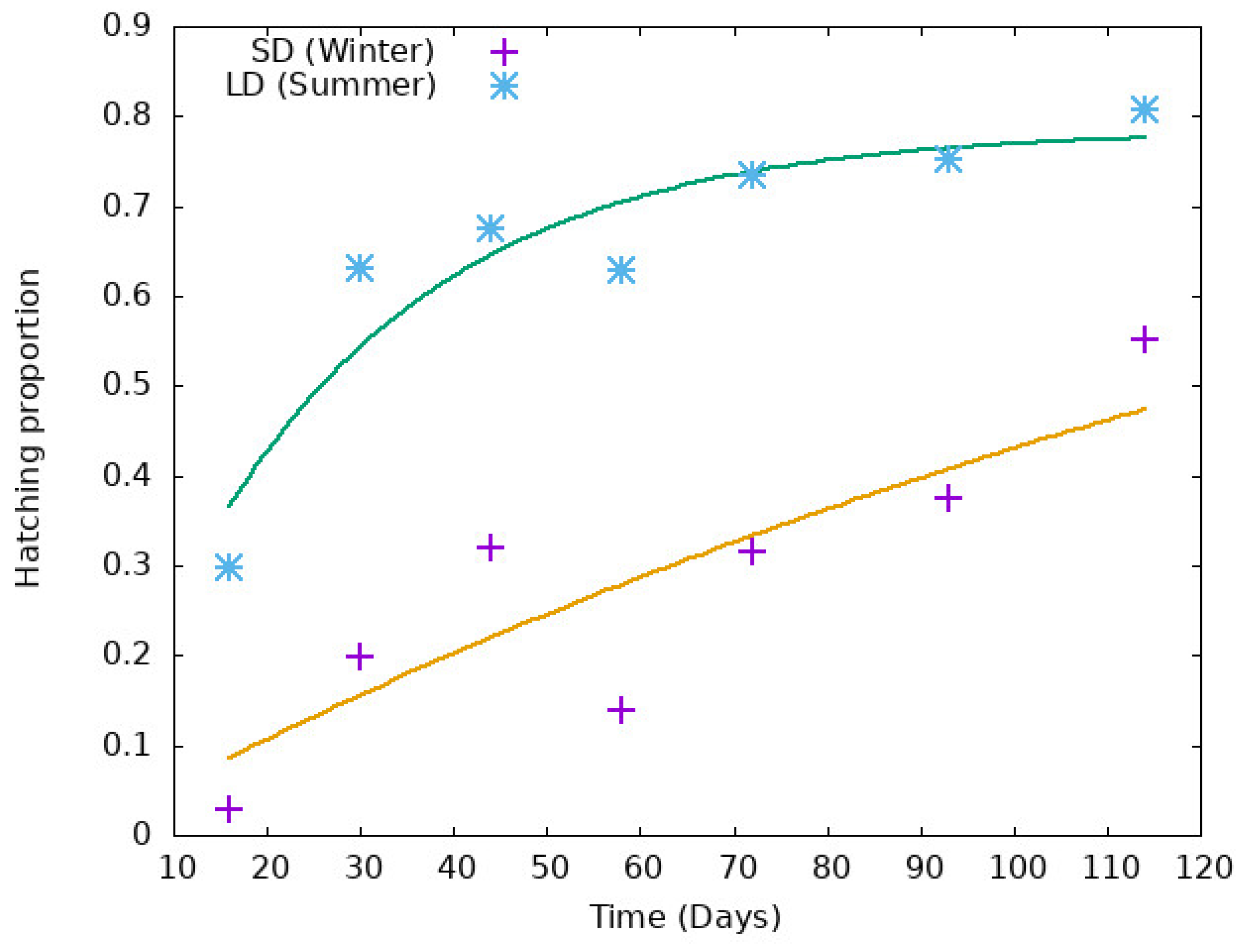
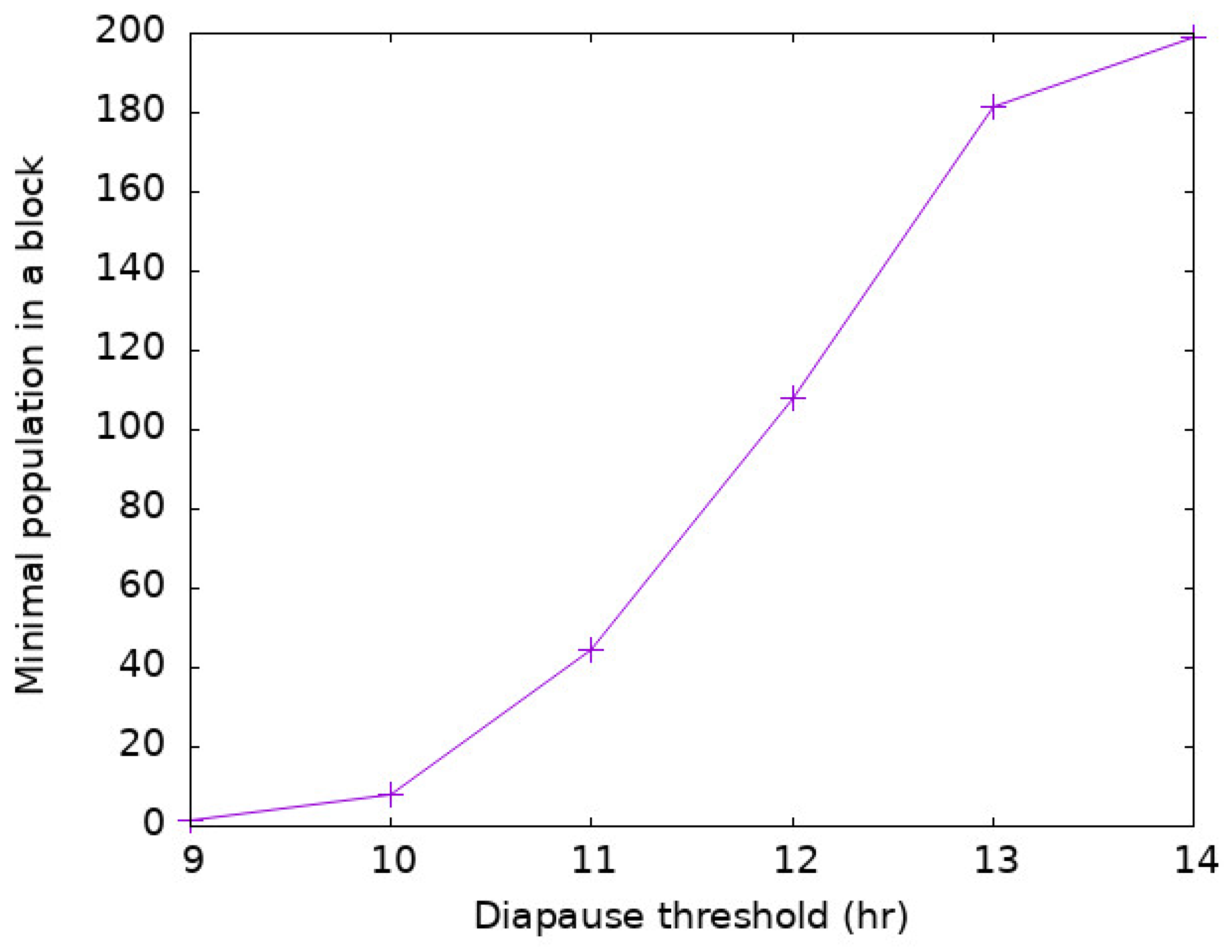
2.3. Modeling Diapause

To model diapause, the eggs laid while the photoperiod was shorter than a given threshold (a parameter to be varied during explorations) were considered to be of the “Short day type” (SD), and those laid while the photoperiod was longer than the threshold corresponded to “Long day type” (LD). According to the elaboration of data from the experiment reported in [16], the two main characteristics that affect the development of the eggs are “dormancy” and “mortality”.
Dormancy corresponds to the proportion of eggs that hatch at the first immersion at time t after they have been laid. Under field conditions, only about 80% of the viable eggs hatch in a first immersion produced between 90 and 180 days after being laid [51]. Thus, we expect the probability of hatching before being laid to be zero (negative times), and to saturate to a value that is smaller than one for very long times. We further assumed that the probability would take the form corresponding to a Poisson process, where the transition between dormancy and readiness to hatch is made with constant probability at constant intervals of time. The model fitted to the data resulted in
f ( t ) = a ( 1 exp ( b t ) )
The result of the fit can be seen for SD and LD eggs in Figure 3.
The mortality rates of the eggs depend as well on the photoperiod during the gonadotropic cycle. The mortality was fitted to the data [48] using the form
f ( t ) = 1 exp ( c t )
The coefficients resulting from the fit are c = 0.0015 ± 13 % (1/day) for SD eggs and c = 0.0039 ± 7 % (1/day) for LD eggs, corresponding to an average longevity of 666 days (SD) and 256 days (LD).

2.4. Direct and Indirect Model Outputs

The output of the model consists of population numbers in each block, and for each stadium in the developmental cycle, as described by the model, as well as the number of events (for example, egg hatching, the transition of larvae between different developmental stages, adults emerged, the flight of adults in each direction from each block, etc.). The time step for the computational model is of 2 hs and finds an upper limit in the event of egg laying, which is associated with dispersal. Food production, food consumption, and the average weights of adults are recorded for every day and block. Random repetitions of 20 runs are usually performed to grasp the influence of random effects.
The output of the model may be further processed through averaging over runs and spatial distribution.
The simulations are usually allowed for three years of transition (July 2008 to June 2011) to lessen the influence of the arbitrary initial condition consisting of a population of 150 LD eggs and 150 SD eggs in every block by 1 July 2008, and with no individuals in any other stage. No sensible changes are observed when initializing the populations with half the number of eggs.

3. Results

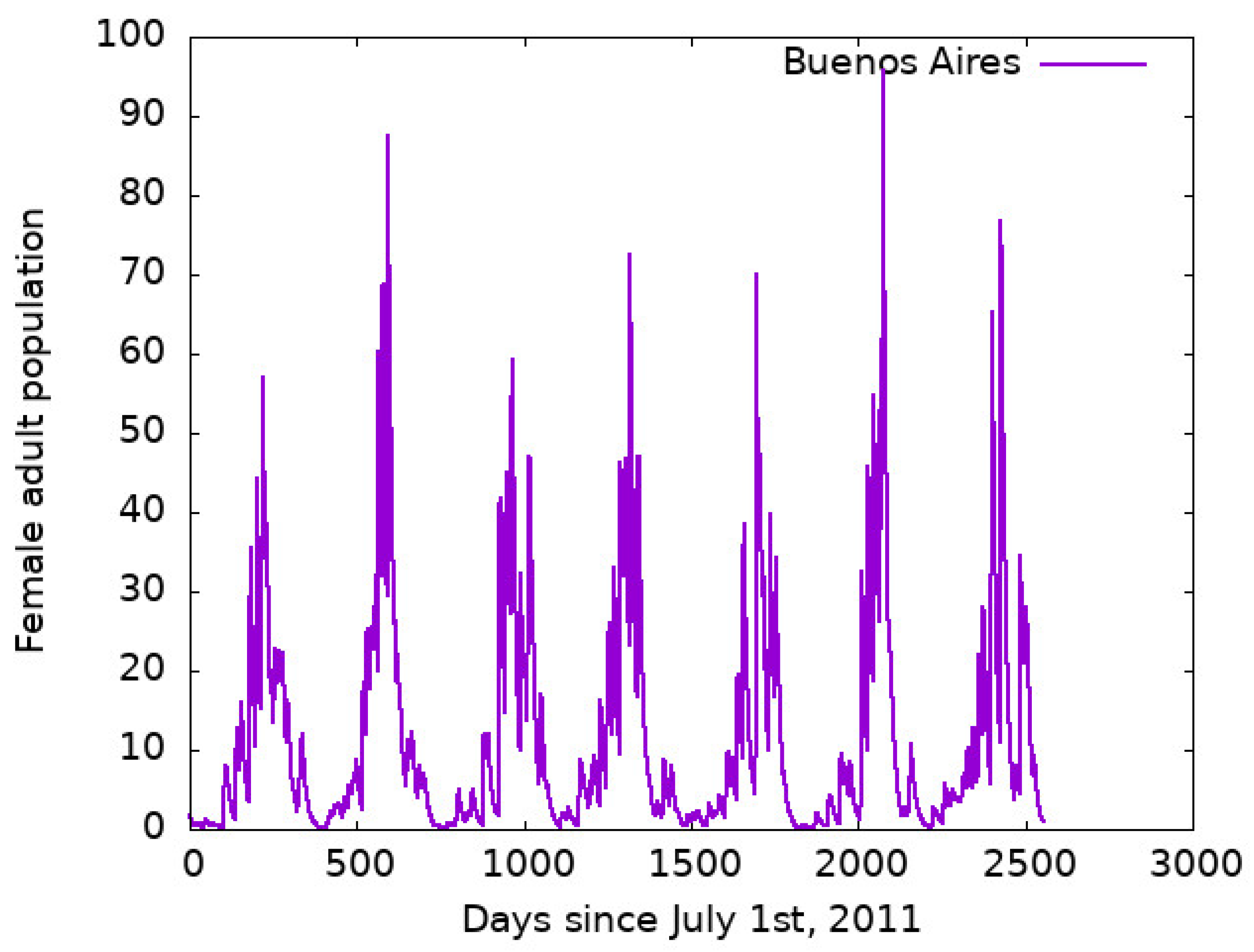
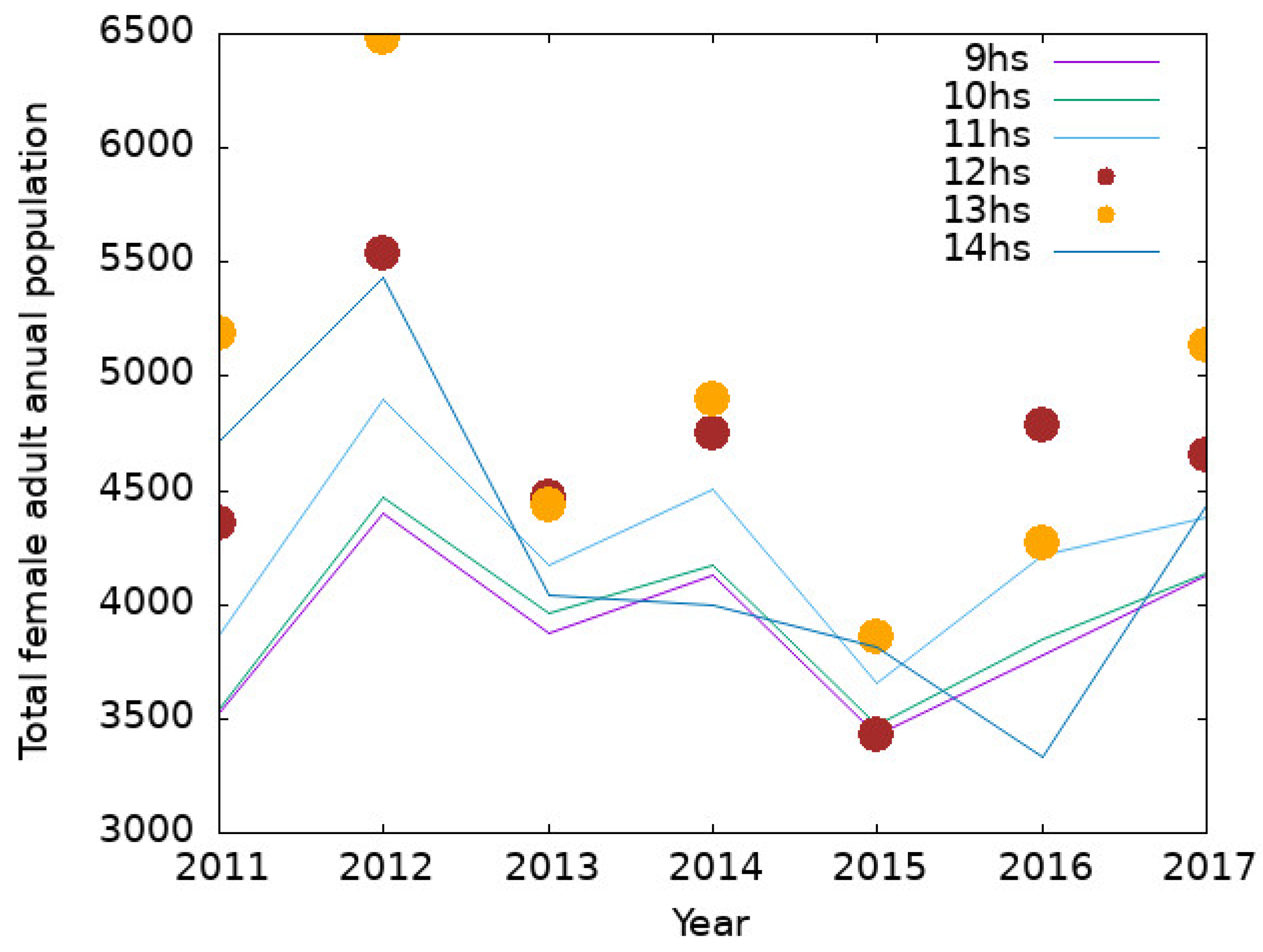
3.1. Outcomes of the Model for Buenos Aires City

During the seven-year simulation (1 July 2011 to 30 June 2018), the adult population presents peaks during the favorable season, decorated by the effect of rains in triggering eclosion; see Figure 4.
During the winter and early spring months, populations of adults Ae. aegypti are only occasionally present. When the temperature conditions become favorable for development, occasional rains induce egg-hatching and reproductive activity starts. The body size of adults evolves during the season (see Appendix C and Figure A3).
The total adult population in the year (evaluated as the sum of female adults during one year of simulation) depends as well on D−Th(see Figure 5).
The threshold of 9 hs corresponds to a situation in which no resistant eggs (SD) are laid, while with a 14 hs threshold, almost all the eggs laid correspond to the resistant type (the largest value of daylight is about 14.5 h). It is important to notice that the higher total (year-round) adult population values are obtained for intermediate D−Th(12 and 13 hs).
The possibility of local extinction (the extinction of all forms of the mosquito in one or several blocks) cannot be ruled out. The minimal population in a block (the lowest value of the total daily population during the year in any of the 60 blocks simulated) reaches values of below five individuals for low D−Thvalues in BA. In addition, extinction in a block is observed with a low probability for a D−Thof 9 hs. The probability is strongly influenced by the breeding sites available and through chance. In Figure 6, we can appreciate how the minimal population in a block (averaged over 20 runs) changes as a function of the threshold value.

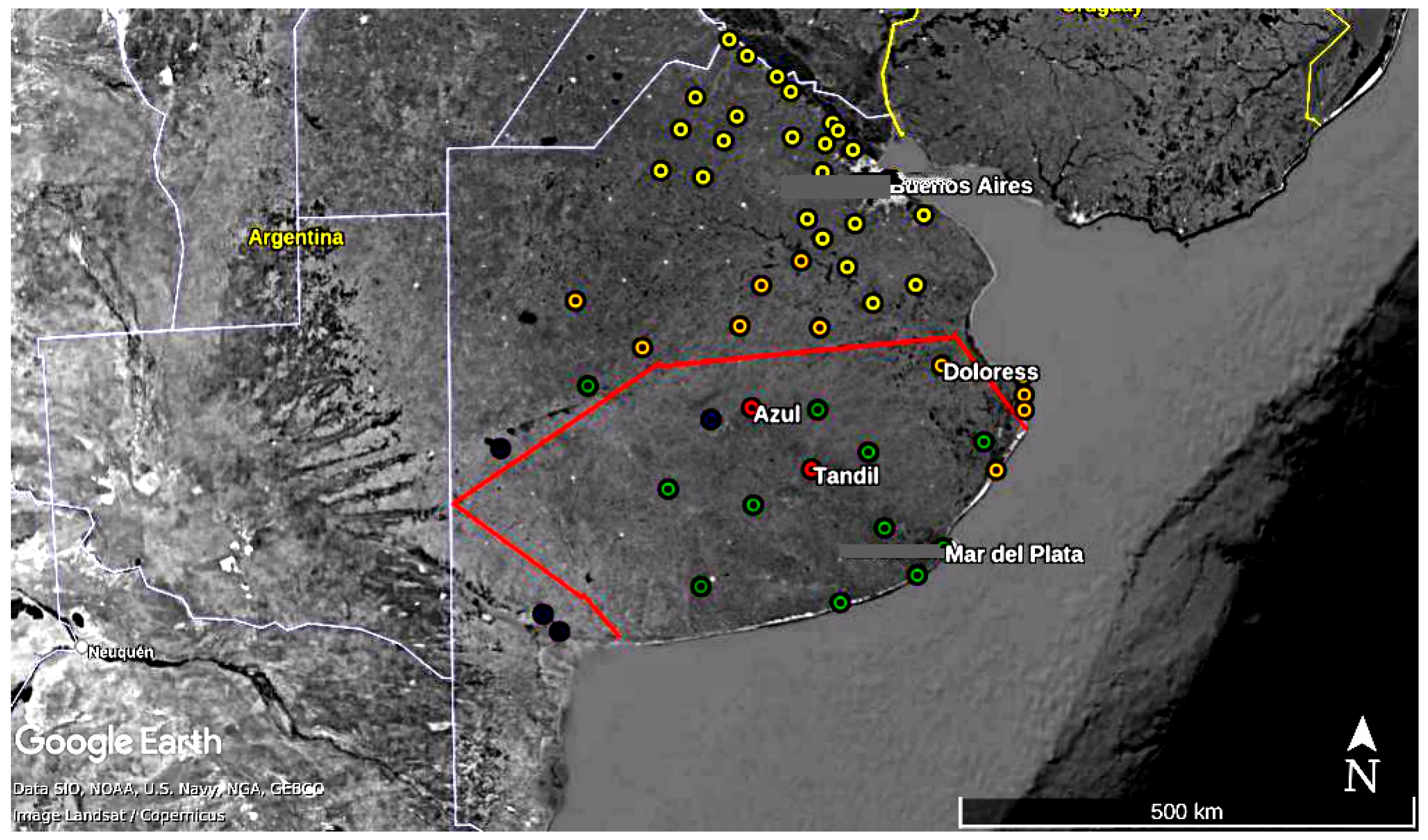
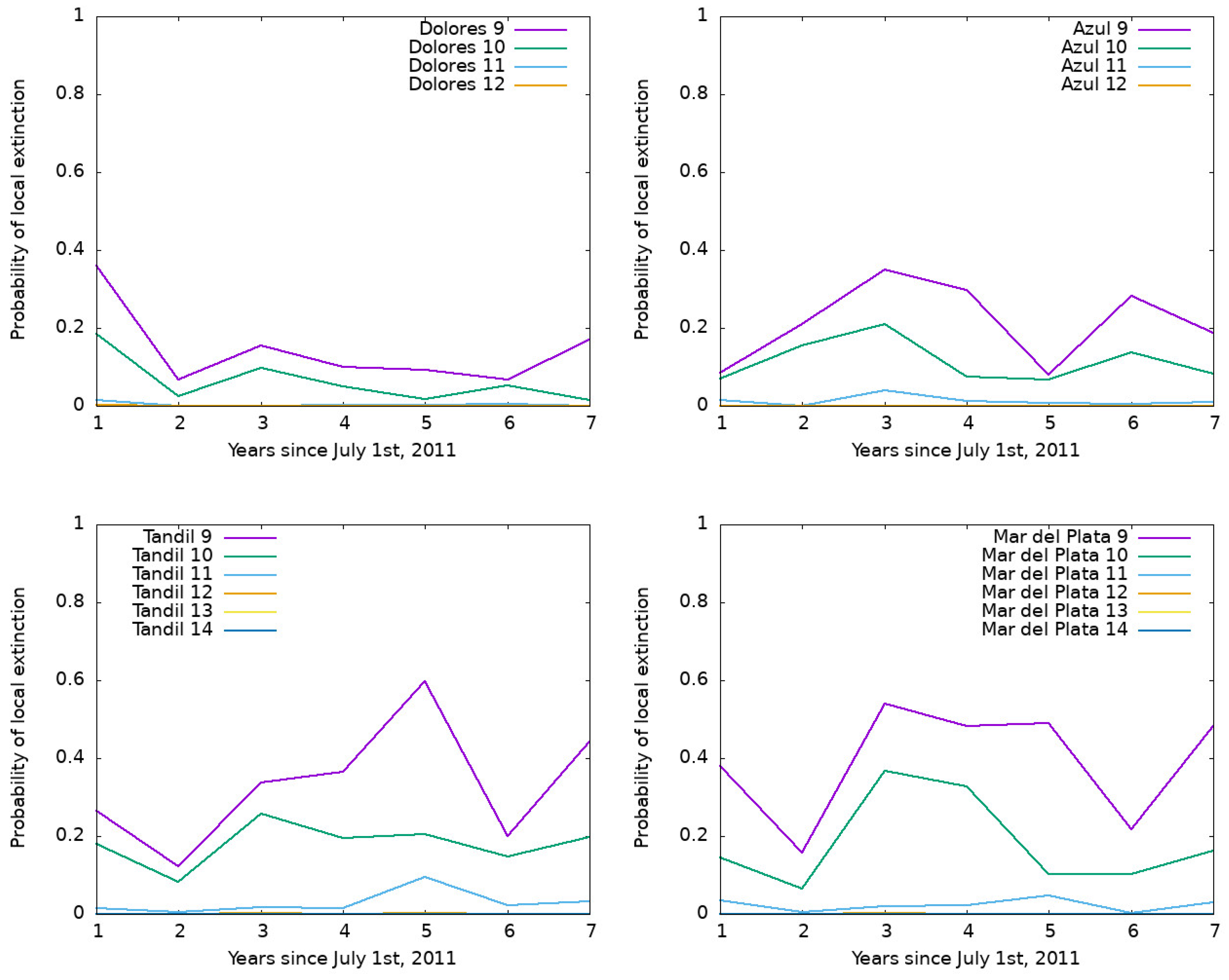
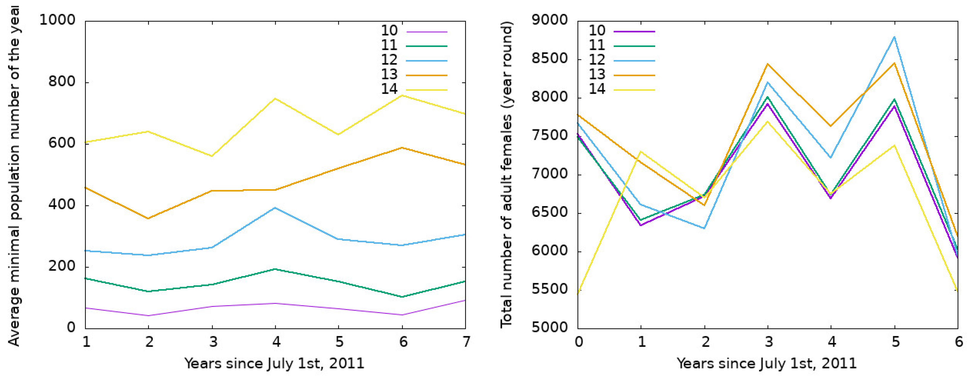
3.2. Output of the Model for Southern Cities in Buenos Aires Province

Four cities: Dolores, Azul, Tandil, and Mar del Plata, have been selected for the study, based upon the availability of weather data and their status with respect to the detection of Ae. aegypti. Of them, Ae. aegypti populations have been reported for Dolores (by health authorities circa 2009–2013 [11]), Tandil [12], and Azul [13]. In contrast, no permanent population has been detected for Mar del Plata where similar searches have been carried out.
The probability of local extinction (the maximum fraction of simultaneously empty blocks of the total simulated blocks) gives an idea on how difficult the results are for the colonization of the landscape. We show the evolution of this probability for the four cities as a function of time during the seven years of simulation (July 2011 to June 2018) in Figure 7.

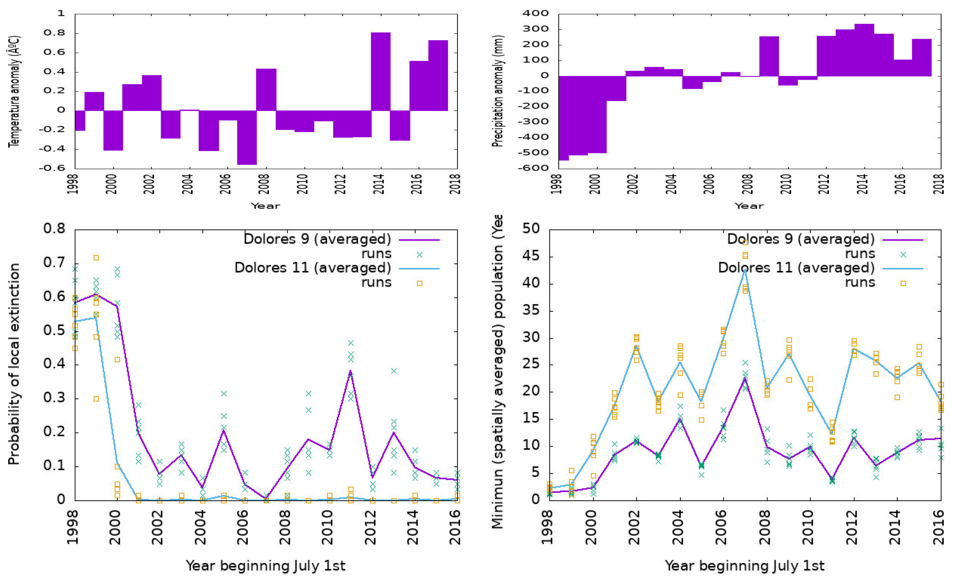
3.3. The 1998–2018 Simulation for Dolores (Buenos Aires)

A 20-year simulation was performed for Dolores covering 10 years of a colder and drier period (on average), followed by a warmer and more rainy 10-year period (the climatic pattern displayed in Figure 8). We notice that in the weather records, there are two important anomalies. The period over 1998–2001 presents an important precipitation defect, and the period of 2014–2017 presents temperatures and precipitations in excess of the average. The dry 1998–2001 period has an important negative impact on the winter populations, as manifested in a substantially larger probability of local extinction and minimally average populations. In contrast, the favorable season of 2014–2017 presents no special features in terms of surviving the winter.

3.4. The Simulation for Resistencia (Chaco)

A simulation for the same period was run using weather and light hours corresponding to the subtropical city of Resistencia in the northern province of Chaco. No local extinction process was detected. We present a minimal year population (spatial average) and a maximal adult year population (spatial average) in Figure 9. Notice that since the hours of day light for Resistencia are in the interval [ 10.40 hs , 13.90 hs ] , we simulate thresholds of 10 hs (all eggs are summer eggs), 11–13 hs, and 14 hs (all eggs are winter eggs).

4. Discussion and Conclusions

The view of modeling advanced in this work corresponds closely to the idea of theory. The aim of a theory is to organize the observations in coherent form, eventually being able to forecast the outcome of different situations from this understanding. In contrast, the most common use of modeling associates it only with forecasting/prediction, and this might promote no understanding at all. With understanding, we mean to provide a layer of accessible observations (experiments) that, logically organized, allow us to form a consistent picture of most (ideally of the totality) of the observations. In the present case, the model has been used to compare the contributions of two different explanatory hypotheses for the phenomena observed. The climatic change explanation has been postulated previously [12] as the only relevant reason for the observations, and we show that this view has no real support.
The colonization of cities in the southern region of temperate South America is a complex series of phenomena that suggests an adaptation of Ae. aegypti to a temperate climate. Complexity is the result of its dependency on climatic factors and on anthropogenic factors such as the availability of breeding sites and long distance transportation by vehicles [52], the dynamics of the nutrients that the species exploits, and the dependence on climatic factors and the physiological behaviors of the mosquito, which we conjecture are subject to adaptive selection. The theory provides a form of separating the different contributions that manifest in nature as a single realization of a unique phenomena. Thus, the role of the theory is to form an analytic tool that is incorporated to the biological research.
Quantitative modeling would require a complete characterization of the mosquito bionomics as a function of the available food and temperature, as well as a reasonable characterization of the environment in terms of the number, quality, and location of breeding sites. However, only parts of this information can be really obtained. The quantitative task is then impossible. What is possible is to use conjectures regarding the information that is not available and to produce qualitative descriptions as a function of the conjectured scenario. In the full region studied, the abundance of breeding sites is a determining factor for the persistence of the species year-round, but this characteristic changes with time, as it is associated with human activity. Moreover, information about breeding sites is also difficult to recollect. For example, a can that is filled with water and placed in the shade under a bush can make a good breeding site, but if the can is moved under direct sunlight, its quality as a breeding site will sharply diminish. This situation represents a serious drawback for the ability to predict, while for the needs of understanding, it is not so relevant. Understanding aims at knowing how populations depend qualitatively on the available breeding site, a functional dependency that does not change with the actual number in such places. In the same form, knowing the precise temperature dependency of the developmental rate is very relevant for prediction, but for our purposes, it is the general tendency that matters. In brief, understanding rests more on quality than on quantity.
With respect to diapause in Ae. aegypti, the emerging picture is that it constitutes a trade-off in which the advantage of more resistant eggs, in terms of surviving the unfavorable season, is obtained at the expense of a longer dormancy. The latter can imply smaller summer adult populations, and then a lesser ability to disperse and to conquer territory. In part, this rationale is demonstrated by the theoretical observation that in BA, the largest adult populations are obtained for intermediate values of the D−Th. However, this is not the only mechanism by which diapause affects the viability of populations. The threshold for diapause changes the relationship between food and larval biomass, resulting in a different temporal progression of pupae into adults as a function of the threshold value. Actually, the body size of the adult mosquitoes is expected to change over the favorable season. The body size is larger at the beginning and smaller towards the end. This is a result of the model that under constant temperature and available food, the adult population tends to be large but of small body size, asymptotically in time. Such an equilibrium favors dispersion without affecting the total biomass much. However, if food develops in the spring time faster than the hatching of the surviving eggs, the relative abundance of food promotes large body sizes (and then, large fecundity) and a shorter developmental time, giving a quick start to the re-population process. As the population growth and the production of food reaches a maximum during the early summer, temperatures then begin to fall. In this process, the food available to each larva diminishes, and consequently, development slows down while the body size diminishes. Thus, the plasticity of body size appears as a beneficial trait for the mosquito under a temperate climate.
Overwintering of the populations represents a challenge and a bottleneck, the overcoming of which is facilitated by diapause. Going from north to south, we observe that winter populations in BA (under the simulated conditions) present very low values (less than five individuals per block), but at these minimal and likely undetectable numbers, they are present in all of the blocks all of the time (see Figure 6). For D−Ththat is equal or larger than 10 to 11 hours, the overwintering shows an improvement, and at the same time, female adult populations are more abundant with values of D−Thin the range of 12 to 13 hs (Figure 5). Thus, we expect a selection pressure that increases D−Thaway from 9 hs and into 10–11 hs. For cities south of BA, in the BAP, the winter bottleneck for Ae. aegypti populations is manifested, as well by the number of blocks with local extinctions (for example, in Dolores).
This situation can be contrasted with that at a subtropical city such as Resistencia (Chaco, AR) (see Figure 9). In the first place, the meaningful range for D−This slightly narrower than that at meridional latitudes. Winter populations are small, but at the same time, they are substantially larger than in BA. Thus, the selective pressure is small. Total (year-round) populations of adult females present low sensitivities to D−Th. We conclude that there is no selective pressure. Displaying diapause is a non-critical help for overwintering, and neutral for dispersion. It is interesting to notice that, while the minimal population increases monotonically with D−Th, this effect is not reflected in the total number of females, which are essentially independent of the threshold. The rationale is that larvae populations, at the end resulting in adult populations, are regulated by the environment in the model by means of available food. Thus, while winter populations are mostly in an egg form, the adults are characteristic of the Summer. The lower mortality of SD eggs influences the winter population noticeably. During the summer, the adult mosquito population tracks the environmental conditions thanks to the large fertility of the mosquito. Thus, the adult populations reach environmental capability (except for the winter conditions displaying extremely low populations, which is not the case for the subtropical city). The environmental capability is in turn independent of the initial conditions in winter.
Overwintering populations south of BA are even smaller (see Figure 7), and local extinction in random blocks occurs in a fashion that depends on the particular year and location. The probability of local extinction for Dolores and Azul may reach the value of 0.35 at a particular year (notice that it is not the same year for Dolores and Azul) for D−Th9 hs. Values of D−Thof 11 hs and above are enough to minimize this effect. In this respect, the situation at Dolores and Azul with D−Thof 11 hs during the winter would be equivalent to the situation at BA with D−Thof 9 hs. It is important to keep in mind that the simulations assume an initial condition in which the area was completely colonized by Ae. aegypti three years before the period simulated.
We will discuss a different case soon. A selective pressure for D−Thof at least 11 hs is greater for Tandil and Mar del Plata than for the previous cases. It is important to notice the difference between Azul and Tandil, both of them being at latitude 36° ± 15′, and Azul being north of Tandil. These small differences would in turn be dramatic for the persistence of Ae. aegypti, if not for the diapause trait.
In the absence of diapause, the model predicts that the chances to colonize Tandil and Mar del Plata are small. The situation is harder (for the mosquito) in Mar del Plata than in Tandil, an observation in the model that is well aligned to the fact that colonies of the mosquito have been observed in Tandil, but not so far in Mar del Plata.
The studied populations of Ae. aegypti in the south of BAP may not constitute a sanitary risk of epidemic outbreaks, since adult populations are limited to a relatively short period of time and are relatively much smaller than those in BA, where dengue has produced outbreaks in the near past [53]. This matter requires a direct approach and it is outside the scope of this work.
Figure 8 allows us to compare between the colder-drier years from 1998 to 2008, and those warmer and rainy years (2009–2018). We see that the overall influence of climatic variability (such as the decennial average temperature) is small. What influences the possibility of the mosquito to become established is mostly the lack of rains during the favorable season, which is characteristic of the 1998–2001 period in the location. The situation is the same, either with negative or positive temperature anomalies. When the temperatures rise (2016–2017), the influence on the probability of extinction at a block is minimal (within the range of fluctuations). In contrast, the effect of diapause is very noticeable.
In conclusion, the articulation of our current knowledge with respect to Ae. aegypti with weather data and geophysical data (light hours) indicate that the mechanism of diapause is the most likely reason for the southward motion of Ae. aegypti, whereas climate change is not. The selective pressure of diapause is weak or absent at the subtropical location studied, and it becomes evident in BA and increases southward.
The “logic” of diapause involves relations with dispersal abilities, weather, and environmental variables such as the availability of breeding sites and the dynamics of food, and it cannot be seen as an independent variable that only affects the overwintering capabilities.
In contrast, “the logic” supporting the influence of climate change is ill constructed since the mosquito does not respond to climatic variables (long-term averages), but rather to weather variables, short-term (season) averages, and the synoptic scale. The length of the unfavorable season is one of the key determining weather features for the ability of the mosquito to move southwards. The sensitivity to a precipitation deficit is far more relevant than the sensitivity to temperature anomalies. However, the anthropic effects during dry periods exert a considerable influence in the populations of Ae. aegypti. With the mosquito being a peridomestic animal, it benefits from people watering and indoor breeding sites [54].
One of the weakest points of the model is its completely conceptual (qualitative) treatment of the foraging of larvae as they affect the breeding environment. There is no biological information on this matter. A sided view has been predominating (perhaps because of practical matters), which emphasizes the influence of the environment on the mosquitoes, but not the reciprocal influences of mosquitoes on their habitats. Yet, from the point of view of modeling and conceptualization, the available food consumed by the larvae (intra-specific competition) is the only regulation of the population size, and other factors such as temperature can create conditions for extinction but not for controlling the overall population size, since temperature acts at the individual level, and then, it is represented by linear transition rates.
Do larvae hatched form SD eggs have the same response times and the same mortality rates compared to larvae hatched from LD eggs? Lacking information, we have assumed so, but since SD eggs are larger than LD eggs, we expect a lower fecundity or a longer gonadotropic cycle for females laying SD eggs. There are no attempts so far at quantifying such effects. Is there a measurable variability of body size along the year, as predicted by the model? These questions exemplify how the necessity of the modeler to give precision to the terms moves them to ask biological questions.

Author Contributions

Conceptualization, H.G.S.; methodology, L.E.A.; software, V.R.A., L.E.A. and H.G.S.; validation, L.E.A., V.R.A. and H.G.S.; formal analysis, L.E.A., V.R.A. and H.G.S.; investigation, L.E.A., V.R.A. and H.G.S.; resources, none; data curation, L.E.A. and H.G.S.; writing—original draft preparation, V.R.A. and H.G.S.; writing—review and editing, L.E.A., V.R.A. and H.G.S.; visualization, none; supervision, H.G.S.; project administration, none; funding acquisition, none. All authors have read and agreed to the published version of the manuscript.

Funding

This research received no external funding.

Data Availability Statement

All data are available from public sources (as indicated in the text), except for a private communication by [48] (indicated as well). A copy of the code is available at Github, https://github.com/hgsolari/AedesBA, accessed on 26 November 2022.

Acknowledgments

We aknowledge fruitful discussions with Sylvia Fischer and the Mosquito Study Group at FCEN-UBA, Argentina.

Conflicts of Interest

The authors declare no conflict of interest.

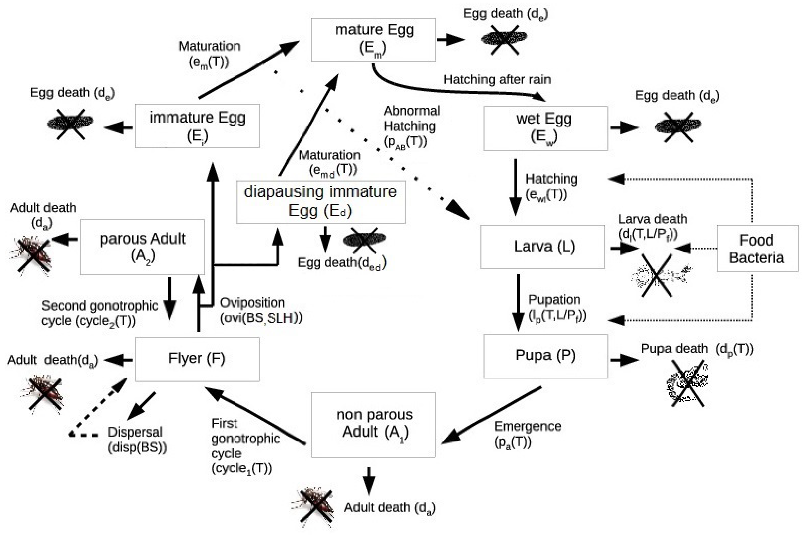
Appendix A. Generalities of the Model

AedesBA is a stochastic model that describes the population dynamics of the Ae. aegypti mosquito. The mathematical structure of the model consists of a Markovian process with non-linear rates. The mechanism regulating the population—intraspecific competition in the larval stage—introduces non-linear growth and feeding rates into the model. Space is explicitly described and is represented by a regular grid. In each unit of the grid, the dynamics of the local population are specified, as well as the interaction between units through the flight of the mosquito.
The model considers the mosquito population at different stages of development. The main stages are egg, larvae, pupa, and adult, and within each of them, different substages are specified, depending on the model version (the details of the version used here are described below). The dynamical evolution of these populations are affected by different events; in general terms, the mortality and the passage to the next stage (next maturation stage, Figure A1). Events occur at rates that depend not only on the population values, but also on temperature. The temperature variation throughout the year introduces a time dependency in the event rates.
Figure A1. Scheme of compartments and events.
Mathematics 10 04510 g0a1
The population evolution follows a Poisson process with the probability that a population state ( E , L , P , A ) (numbers of: eggs = E, larves = L, pupae = P and adults = A) evolves over time according to a Kolmogorov forward equation. The implemented numeric simulation considers a Poisson approximation for fixed times [39]. Basically, the idea is: given X ( t ) = ( E , L , P , A ) ( t ) , a vector with integer variables representing the population at time t, and given the quantities e i ( i = 1 k ) that denote the events in which the populations change by a fixed amount Δ i , the stochastic process can be written as [55]
X ( t ) = X ( 0 ) + i = 1 k Δ i Y ( w i ) ,
where w i ( X ) is the transition rate of the i-th event and Y is a stochastic Poisson process with rate w. The probability that n i events of type i have occurred between time t and time t + d t is approximated by a Poisson distribution with parameter λ i . Therefore, the probability that the population takes the value
X t + d t = X ( t ) + i = 1 k Δ i n i
is approximated by the product of independent Poisson distributions of the form
P ( n 1 , n 2 , , n k , t + dt X ( t ) ) = i = 1 k Prob ( λ i ) .
Then, a differential equation for λ is obtained
d λ i d t = < w i ( x ) >
Consider as an example the population of pupae. Using Equation (A1), we have that P ( t + d t ) = P ( t ) + n P n P A n M P , where n L , n P , n M P are stochastic variables that respectively represent the number of pupations, the number of adults emerged, and the number of pupae deaths, having a place during a window of time d t . The values of the variables n i are obtained by generating a stochastic number from a Poisson distribution with a mean of λ i . Of course, a system of coupled differential equations given by Equation (A1) has been solved previously to obtain the λ i values, as explained in [39]. Therefore, if we know the population at a time t, we can obtain the population at a posterior time t + d t .

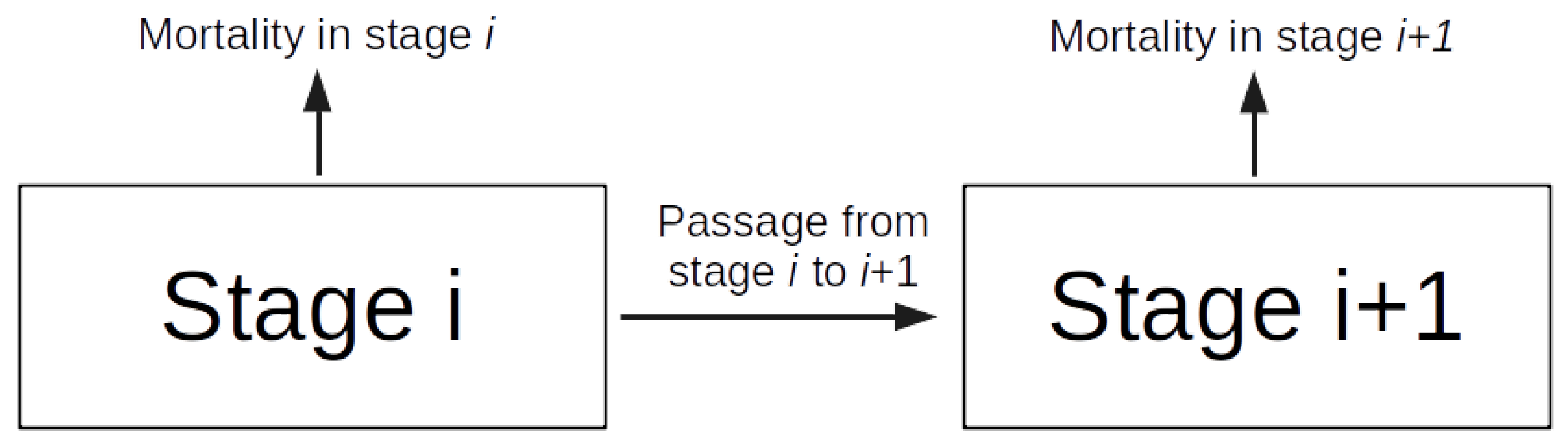
Phases within the Main Ae. aegypti Stages and Rates

Adults. Within this stage, the model differentiates three phases (see details in Otero, 2008):
  • Female adults not having laid eggs, A 1 (longer gonadotropic cycle).
  • Female adults having laid eggs, A 2 (shorter gonadotropic cycle).
  • Flyers, F. Females are able to deposit their eggs; they fly in order to find oviposition sites. This stage is responsible for the connection between blocks. The flyers can only relocate to neighboring units.
Pupa. We define 22 sub-stages within the pupae. These 22 phases are not regular entomological classifications, but they follow the results of laboratory experiments of larvae raised under different nutrients scenarios [28]. The rates to go through these sub-stages are equal, independent of the food level, and depend on temperature. The same is true for the death rates.
Larvae. The molting of chitinous skin defines four substages within larvae. However, AedesBA distinguishes 67 sub-stages according to the same experimental results used to define the pupa stages [28]. Since larvae are the only immature stage that feeds, the rates to pass the 67 sub-stages are classified in two categories: seven depend on food availability and temperature, and 60 only on temperature. Within each category, the rates are the same. The mortality rates in each of the 67 sub-stages become the same and depend on temperature and food level.
Eggs. AedesBA considers six different populations within the egg stage. SD and LD eggs have three sub-stages each [16].
  • Immature eggs, E 1 (eggs laid by females),
  • Mature eggs, E 2 ,
  • Wet eggs, E 3 .
Eggs are laid immature, and depending on the time of the year (on the photoperiod), they will be affected by the diapause effect. Depending on the temperature, immature eggs become mature. Then, as a result of rainfall, the eggs become wet and can hatch. The model considers a rainfall threshold of 7.5 mm for all eggs to become wet, since Ae. aegypti lays its eggs just above the water level.
Food for larvae. The larvae of Ae. aegypti feed on bacteria or yeast associated with the decomposition of organic matter, mainly by filtering water [56]. Correspondingly, we assume that the larvae forage on stranded bacteria, without altering the decomposition process. Food, f, is produced at a rate f P R that depends on temperature T. While food is available, it evolves with the following equation:
d f d t + u f = f P R ( T ) f B L
where u is a characteristic decay time for the food and B L is the food consumed by the larvae in the breeding site. For details, see [42]. Food production is modeled with temperature as bacteria using a Ratkowsky-2 model [20,57]
Body size. The body sizes of the larval populations evolve according to a von Bertalanffy [58] equation for each stage. The equation was taken as
d B i d t = μ B i log B i B i ( )
where B is the body size, μ is a scaling of time that depends on the available food fitted to the laboratory experimental results, and B ( ) is an asymptotic body size adjusted with growth data in [6]. The rate of food consumption is
B L = i ( B i L i ) f
where the sum ranges over all the larvae stages and represents the consumption by all of the present biomass of larvae in the breeding site. This is actually the only non-linear element in the model.

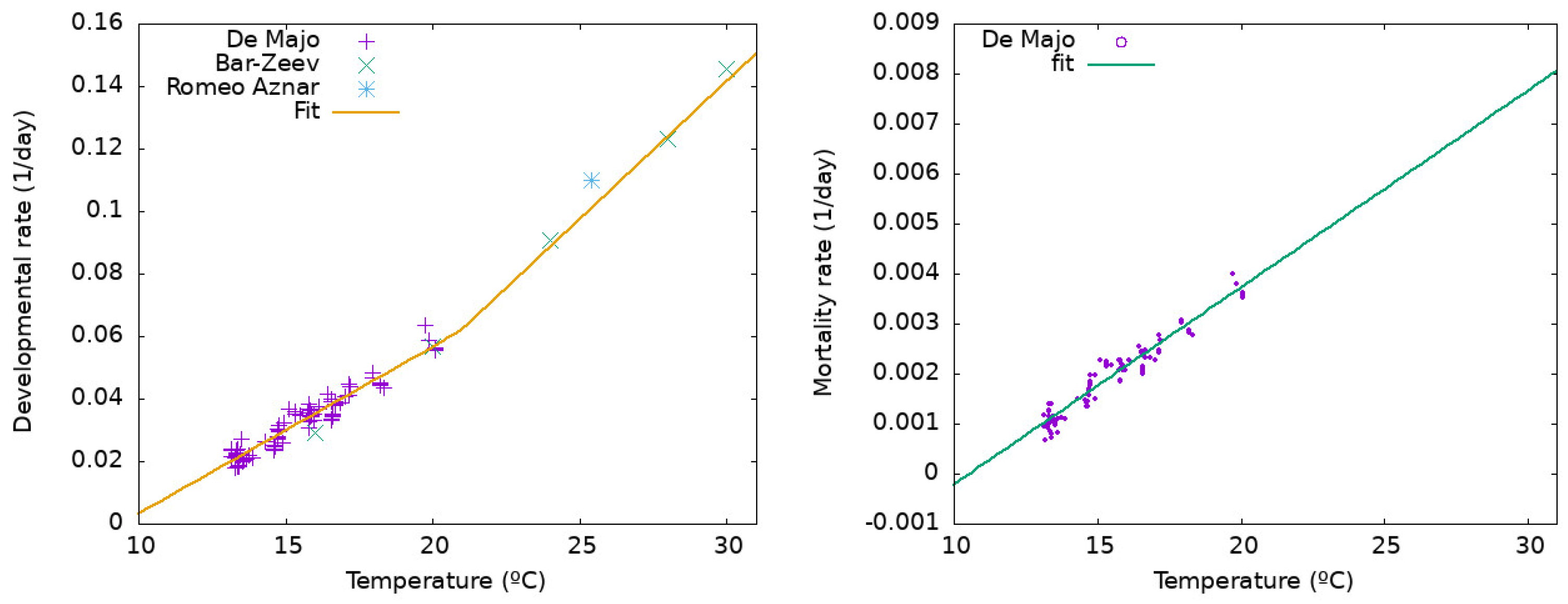
Appendix B. Temperature Dependence of Development and Mortality as a Function of Temperature

The dependence of the developmental rate and, to a lesser extent, the mortality rate with respect to temperature, in immature stages, has been a topic that has been addressed repeatedly in the literature ever since the pioneering work by Bar-Zeev [59]. A comparison between the results in [59] and those in [15] at the same temperature (~16 °C) indicate an agreement within the uncertainty of the measurements. The data point corresponding to [29] is also well aligned. In all these experiments, the provided food was replaced periodically to decouple the time evolution of nutrients from the physiological traits. The range of temperature in the latter is 10–20 °C. In turn, in the former is 16–38 °C, while the range of temperature needed for our simulations covers the range of 10–31 °C.
The developmental and mortality rates were assumed to be a product of the form
r ( F , T ) = r 26 ( F ) r o ( T )
where r 26 ( F ) is the dependence on the available food measured in [27] at ~26 °C, and r o ( T ) is the dependence on temperature under the optimal feeding conditions reported in [15,59].
The developmental rate (the inverse of the average developmental time in days) can be represented by the continuous function
r o ( T ) = 0 T 9.49 ° C 0.0503 + 0.0053 ( 1 / ° C ) T 9.49 ° C < T 21 ° C 0.0088 ( 1 / ° C ) ( T 21 ° C ) + 0.0619 21 ° C < T 31 ° C
resulting from the fit displayed in Figure A2. Notice that a rate of 0 ( 1 / day ) represents an infinite amount of time required to develop, and no successful development is possible under 9.49 ± 5 % ° C .
Figure A2. Developmental rate (left) and mortality (right) fitted as a function of temperature for optimal food conditions.
Mathematics 10 04510 g0a2
The experiments do not report the mortality rate directly, but rather the frequency (probability) of death during the developmental period. In terms of the model, death is the result from a sequence of N = 89 Poisson races [38] that cover the N developmental stages that the model uses to produce the proper statistical distribution of developmental times. Let R d = 1 < t d > be the developmental rate per stage ( < t d > stands for the average time in the stage), R m the mortality rate, and P m the mortality probability (frequency); the relation is
1 P m = R d R d + R m N
Thus, the mortality rate, given the survival probability ( 1 P m ) = P s , is
P s 1 / N 1 < t d > = R m
which suggests the regression displayed in the right panel of Figure A2, which in numerical values is
R m = ( 0.00415 + T 0.00039 ( 1 / ° C ) ) ( 1 / day )
for T 10 ° C . It is worth noticing that the mortality rate increases with temperature; despite the decrease in the death probability, it simply means that the developmental time decreases with temperature faster than the probability of death.

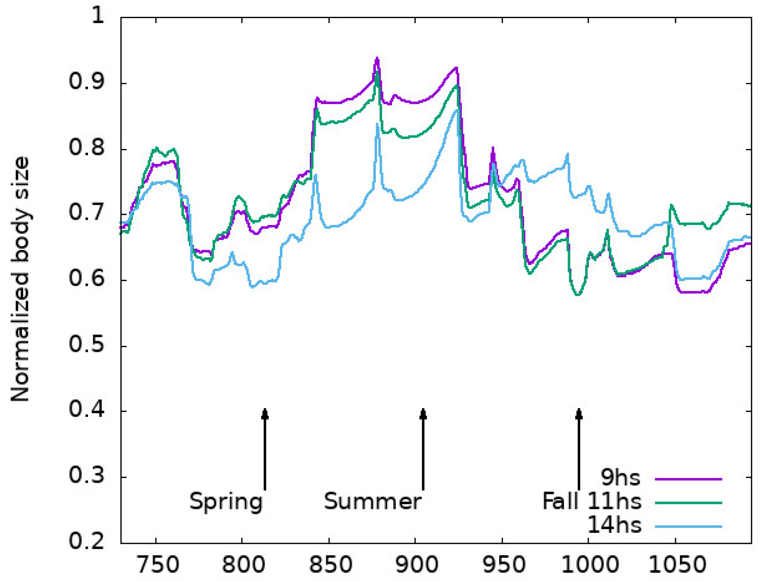
Appendix C. Body Size Evolution

Body size is ultimately regulated by the relation between available food and the biomass of larvae. Large body sizes correspond to abundant food for each larvae, it is also associated with a short developmental time. In Figure A3, the threshold of 9 hs corresponds to a situation in which no resistant eggs (SD) are laid, while with a 14 hs threshold, almost all of the eggs laid correspond to the resistant type (the largest value of daylight is about 14.5 h). It is important to notice that in general, the body size is large at the beginning of the favorable season and decreases later in the season.
Figure A3. Normalized body size according to the model for the year starting on 1 July 2012. Simulations with D−Thof 9, 11, and 14 hs.The normalization corresponds to the largest physiologically possible body size according to the model. Arrows indicate the beginning of the season. The details of the pattern are sensible to the the relation between larvae foraging and body growth, which is not well known.
Mathematics 10 04510 g0a3

References

  1. Agramonte, A. An Account of Dr. Louis-Daniel Beauperthuy: A Pioneer in Yellow Fever Research. Boston Med. Surg. J. 1908, CLV111, 928–929. [Google Scholar] [CrossRef] [Green Version]
  2. Finlay, C. Yellow Fever: Its Transmission By Means of the Culex Mosquito. Am. J. Med. Sci. 1886, 184, 395–408. [Google Scholar] [CrossRef]
  3. Finlay, C.J. Mosquitoes considered as transmitters of yellow fever and malaria. Psyche 1899, 8, 379–384. [Google Scholar] [CrossRef]
  4. Reed, W.; Carroll, J.; Agramonte, A.; Lazear, J.W. The Etiology of Yellow Fever—A Preliminary Note. Public Health Pap. Rep. 1900, 26, 37–53. [Google Scholar]
  5. Carter, H.R. Yellow Fever: An Epidemiological and Historical Study of Its Place of Origin; The Williams & Wilkins Company: Baltimore, MD, USA, 1931. [Google Scholar]
  6. Christophers, R. Aedes aegypti (L.), the Yellow Fever Mosquito; Cambridge University Press: Cambridge, UK, 1960. [Google Scholar]
  7. WHO. Dengue Hemorrhagic Fever. Diagnosis, Treatment, Prevention and Control, 2nd ed.; World Health Organization: Geneva, Switzerland, 1998.
  8. FUNCEI. Dengue enfermedad emergente. Fund. Estud. Infectológicos 1999, 2, 1–12. [Google Scholar]
  9. Otero, M.; Solari, H.G.; Schweigmann, N. A Stochastic Population Dynamic Model for Aedes aegypti: Formulation and Application to a City with Temperate Climate. Bull. Math. Biol. 2006, 68, 1945–1974. [Google Scholar] [CrossRef]
  10. Curto, S.; Boffi, R.; Carbajo, A.E.; Plastina, R.; Schweigmann, N.; Salomón, O. Reinfestación del territorio argentino por Aedes aegypti. Distribución geográfica (1994–1999). In Actualizaciones en Artropodología Sanitaria Argentina; Salomón, O., Ed.; Fundación Mundo Sano: Buenos Aires, Argentina, 2002; pp. 127–137. [Google Scholar]
  11. Zanotti, G.; Majo, D.; Sol, M.; Alem, I.; Schweigmann, N.; Campos, R.E.; Fischer, S. New records of Aedes aegypti at the southern limit of its distribution in Buenos Aires province, Argentina. J. Vector Ecol. 2015, 40, 408–411. [Google Scholar] [CrossRef]
  12. Carbajo, A.; Cardo, M.; Vezzani, D. Past, present and future of Aedes aegypti in its South American southern distribution fringe: What do temperature and population tell us? Acta Trop. 2019, 190, 149–156. [Google Scholar] [CrossRef]
  13. Rubio, A.; Cardo, M.V.; Vezzani, D.; Carbajo, A.E. Aedes aegypti spreading in South America: New coldest and southernmost records. Mem. Inst. Oswaldo Cruz 2020, 115, e190496. [Google Scholar] [CrossRef]
  14. Byttebier, B.; De Majo, M.S.; Fischer, S. Hatching response of Aedes aegypti (Diptera: Culicidae) eggs at low temperatures: Effects of hatching media and storage conditions. J. Med. Entomol. 2014, 51, 97–103. [Google Scholar] [CrossRef] [Green Version]
  15. De Majo, M.S.; Montini, P.; Fischer, S. Egg hatching and survival of immature stages of Aedes aegypti (Diptera: Culicidae) under natural temperature conditions during the cold season in Buenos Aires, Argentina. J. Med. Entomol. 2017, 54, 106–113. [Google Scholar] [CrossRef]
  16. Fischer, S.; De Majo, M.S.; Di Battista, C.M.; Montini, P.; Loetti, V.; Campos, R.E. Adaptation to temperate climates: Evidence of photoperiod-induced embryonic dormancy in Aedes aegypti in South America. J. Insect Physiol. 2019, 117, 103887. [Google Scholar] [CrossRef]
  17. Mensch, J.; Di Battista, C.; De Majo, M.S.; Campos, R.E.; Fischer, S. Increased size and energy reserves in diapausing eggs of temperate Aedes aegypti populations. J. Insect Physiol. 2021, 131, 104232. [Google Scholar] [CrossRef]
  18. Gillett, J.D. Control of Hatching in Prediapause Eggs of Aedes Mosquitoes. Nature 1959, 104, 1621–1623. [Google Scholar] [CrossRef]
  19. Hanson, S.M.; Craig, G.B., Jr. Cold acclimation, diapause, and geographic origin affect cold hardiness in eggs of Aedes albopictus (Diptera: Culicidae). J. Med. Entomol. 1994, 31, 192–201. [Google Scholar] [CrossRef]
  20. Zwietering, M.H.; de Koos, J.T.; Hasenack, B.E.; de Witt, J.C.; van’t Riet, K. Modeling of bacterial growth as a function of temperature. Appl. Environ. Microbiol. 1991, 57, 1094–1101. [Google Scholar] [CrossRef] [Green Version]
  21. Gillett, J.D. Variation in the Hatching-Response of Aedes Eggs (Diptera: Culicidae). Bull. Entomol. Res. 1955, 46, 241–254. [Google Scholar] [CrossRef]
  22. Gillett, J.D. The Inherited Basis of Variation in the Hatching Response of Aedes Eggs (Diptera: Culicidae). Bull. Entomol. Res. 1955, 46, 255–265. [Google Scholar] [CrossRef]
  23. Gillett, J.D.; Roman, E.A.; Phillips, V. Erratic Hatching in Aedes Eggs: A New Interpretation. Proc. R. Soc. Lond. B 1977, 196, 223–232. [Google Scholar]
  24. Carbajo, A.E.; Gomez, S.M.; Curto, S.I.; Schweigmann, N. Variación Espacio Temporal del Riesgo de Transmisión de Dengue en la Ciudad de Buenos Aires. Medicina 2004, 64, 231–234. [Google Scholar]
  25. Otero, M.; Schweigmann, N.; Solari, H.G. A stochastic spatial dynamical model for Aedes aegypti. Bull. Math. Biol. 2008, 70, 1297–1325. [Google Scholar] [CrossRef] [PubMed]
  26. Legros, M.; Otero, M.; Romeo Aznar, V.; Solari, H.; Gould, F.; Lloyd, A.L. Comparison of two detailed models of Aedes aegypti population dynamics. Ecosphere 2016, 7, e01515. [Google Scholar] [CrossRef] [PubMed]
  27. Romeo Aznar, V. Biología teórica, modelo y experimentos aplicados al entendimiento de la dinámica poblacional del mosquito Aedes aegypti. Ph.D. Thesis, Facultad de Ciencias Exactas y Naturales, Universidad de Buenos Aires, Buenos Aires, Argentina, 2015. [Google Scholar]
  28. Romeo Aznar, V.; De Majo, M.S.; Fischer, S.; Natiello, M.A.; Solari, H.G. A model for the development of Aedes (Stegomyia) aegypti (and other insects) as a function of the available food. J. Theor. Biol. 2015, 365, 311–324. [Google Scholar] [CrossRef] [PubMed]
  29. Romeo Aznar, V.; Alem, I.; De Majo, M.S.; Byttebier, B.; Solari, H.G.; Fischer, S. Effects of scarcity and excess of larval food on life history traits of Aedes aegypti (Diptera: Culicidae). J. Vector Ecol. 2018, 43, 117–124. [Google Scholar] [CrossRef]
  30. Focks, D.A.; Haile, D.C.; Daniels, E.; Moun, G.A. Dynamics life table model for Aedes aegypti: Analysis of the literature and model development. J. Med. Entomol. 1993, 30, 1003–1018. [Google Scholar] [CrossRef] [PubMed]
  31. Focks, D.A.; Haile, D.C.; Daniels, E.; Mount, G.A. Dynamic life table model for Aedes aegypti: Simulations results. J. Med. Entomol. 1993, 30, 1019–1029. [Google Scholar]
  32. Kant, I. The Critique of Pure Reason; Meiklejohn, J.M.D., Translator; An Electronic Classics Series Publication; Manis, J., Ed.; PSU-Hazleton: Hazleton, PA, USA, 2010. [Google Scholar]
  33. Whewell, W. The History of Scientific Ideas, 3rd ed.; JW Parker: London, UK, 1858; Volume 1. [Google Scholar]
  34. Peirce, C. Collected Papers of Charles Sanders Peirce; InteLex Corporation: Charlottesville, VA, USA, 1994. [Google Scholar]
  35. Piaget, J.; García, R. Psicogénesis e Historia de la Ciencia; Siglo XXI: Madrid, Spain, 1982. [Google Scholar]
  36. von Goethe, J. The Maxims and Reflections of Goethe; The MacMillan Company: London, UK, 1906. [Google Scholar]
  37. Solari, H.G.; Natiello, M. Science, Dualities and the Fenomenological Map. Found. Sci. 2022. [Google Scholar] [CrossRef]
  38. Durrett, R. Essentials of Stochastic Processes; Springer: New York, NY, USA, 2001. [Google Scholar]
  39. Solari, H.G.; Natiello, M.A. Stochastic Population Dynamics: The Poisson Approximation. Phys. Rev. E 2003, 67, 031918. [Google Scholar] [CrossRef] [PubMed] [Green Version]
  40. Bergero, P.; Ruggerio, C.; Lombardo, R.; Schweigmann, N.; Solari, H. Dispersal of Aedes aegypti: Field study in temperate areas and statistical approach. J. Vector Borne Dis. 2013, 50, 163–170. [Google Scholar] [CrossRef]
  41. Romeo Aznar, V. El Efecto de la Lluvia sobre la Eclosión de Huevos de Aedes aegypti. Estudio e Incorporación a un Modelo. Master’s Thesis, Departamento de Física, Universidad de Buenos Aires, Buenos Aires, Argentina, 2010. [Google Scholar]
  42. Romeo Aznar, V.; Otero, M.J.; de Majo, M.S.; Fischer, S.; Solari, H.G. Modelling the Complex Hatching and Development of Aedes aegypti in Temperated Climates. Ecol. Model. 2013, 253, 44–55. [Google Scholar] [CrossRef]
  43. Powell, J. Genetic Variation in Insect Vectors: Death of Typology? Insects 2018, 9, 139. [Google Scholar] [CrossRef] [PubMed] [Green Version]
  44. Otero, M.; Solari, H.G. Mathematical model of dengue disease transmission by Aedes aegypti mosquito. Math. Biosci. 2010, 223, 32–46. [Google Scholar] [CrossRef] [PubMed]
  45. Focks, D.A.; Haile, D.C.; Daniels, E.; Keesling, D. A simulation model of the epidemiology of urban dengue fever: Literature analysis, model development, preliminary validation and samples of simulation results. Am. J. Trop. Med. Hyg. 1995, 53, 489–505. [Google Scholar] [CrossRef] [PubMed]
  46. Seijo, A.; Romer, Y.; Espinosa, M.; Monroig, J.; Giamperetti, S.; Ameri, D.; Antonelli, L. Brote de Dengue Autóctono en el Area Metropolitana Buenos Aires. Experiencia del Hospital de Enfermedades Infecciosas F. J. Muñiz. Medicina 2009, 69, 593–600. [Google Scholar]
  47. Fernández, M.L.; Otero, M.; Schweigmann, N.; Solari, H.G. A mathematically assisted reconstruction of the initial focus of the yellow fever outbreak in Buenos Aires (1871). Pap. Phys. 2013, 5, 050002. [Google Scholar] [CrossRef] [Green Version]
  48. Fischer, S.; Departamento de Ecología, Genética y Evolución, FCEN-UBA. Private Communication, 2018.
  49. Duffie, J.A.; Beckman, W.A. Solar Engineering of Thermal Processes, 4th ed.; Wiley: Hoboken, NJ, USA, 2013. [Google Scholar]
  50. Grech, M.G.; Ludueña-Almeida, F.; Almirón, W.R. Bionomics of Aedes aegypti subpopulations (Diptera: Culicidae) from Argentina. J. Vector Ecol. 2010, 35, 277–285. [Google Scholar] [CrossRef]
  51. Fischer, S.; Alem, I.S.; De Majo, M.S.; Campos, R.E.; Schweigmann, N. Cold season mortality and hatching behavior of Aedes aegypti L.(Diptera: Culicidae) eggs in Buenos Aires City, Argentina. J. Vector Ecol. 2011, 36, 94–99. [Google Scholar] [CrossRef] [Green Version]
  52. Ayala, A.M.; Vera, N.S.; Chiappero, M.B.; Almirón, W.R.; Gardenal, C.N. Urban Populations of Aedes aegypti (Diptera: Culicidae) From Central Argentina: Dispersal Patterns Assessed by Bayesian and Multivariate Methods. J. Med. Entomol. 2020, 57, 1069–1076. [Google Scholar] [CrossRef] [Green Version]
  53. Tittarelli, E.; Lusso, S.B.; Goya, S.; Rojo, G.L.; Natale, M.I.; Viegas, M.; Mistchenko, A.S.; Valinotto, L.E. Dengue Virus 1 Outbreak in Buenos Aires, Argentina, 2016. Emerg. Infect. Dis. 2017, 23, 1684. [Google Scholar] [CrossRef]
  54. Barrera, R.; Amador, M.; MacKay, A.J. Population dynamics of Aedes aegypti and dengue as influenced by weather and human behavior in San Juan, Puerto Rico. PLoS Neglected Trop. Dis. 2011, 5, e1378. [Google Scholar] [CrossRef] [PubMed] [Green Version]
  55. Ethier, S.N.; Kurtz, T.G. Markov Processes; John Wiley and Sons: New York, NY, USA, 1986. [Google Scholar]
  56. Merritt, R.W.; Dadd, R.H.; Walker, E.D. Feeding behavior, natural food, and nutritional relationships of larval mosquitoes. Annu. Rev. Entomol. 1992, 37, 349–376. [Google Scholar] [CrossRef] [PubMed]
  57. Zwietering, M.H.; de Wit, J.C.; Cuppers, H.G.; van’t Riet, K. Modeling of bacterial growth with shifts in temperature. Appl. Environ. Microbiol. 1994, 60, 204–213. [Google Scholar] [CrossRef] [Green Version]
  58. von Bertalanffy, L. Principles and theories of growth. In Fundamental Aspects of Normal and Malignant Growth; Nowinski, W., Ed.; Elsevier: Amsterdam, The Netherlands, 1960. [Google Scholar]
  59. Bar-Zeev, M. The effect of temperature on the growth rate and survival of the immature stages of Aedes aegypti. Bull. Entomol. Res. 1958, 49, 157–163. [Google Scholar] [CrossRef]
Figure 1. Evolution of the southern limit for Ae. aegypti distribution after Curto et al. [10], Zanotti et al. [11], Carbajo et al. [12], Rubio et al. [13]. The red line indicates approximately the 15 °C annual isotherm. Green cities: Ae. aegypti not found. Red: reports from 2019–2020. Dark blue: Municipal reports. Orange: 2013–2015. Yellow: before 2013.
Mathematics 10 04510 g001
Figure 2. Life cycle of Ae. aegypti, as described in the model AedesBA, with the subpopulations and rates. The rates can depend on temperature (T), daily sunlight hours (SLH), numbers of breeding sites (BS), and the quotient between larvae and food production (L/Pf). The population cycle, as described in Appendix A, goes through three egg forms labeled ( E , E m , E w ). For each egg population in {SD, LD}, the larvae stages L progress until pupa, P. After metamorphosis of the pupae, non-parus adult females emerge, A 1 (males are considered implicitly). Females become F; when seeking oviposition sites and after the first laying of eggs, they become parus, A 2 . In all of the stages of the life cycle, there is a death event competing with progression in the life cycle.
Mathematics 10 04510 g002
Figure 3. Long day-type eggs present a dormancy characterized by the function f ( t ) = ( 0.785 ± 6 % ( 1 exp ( 0.039 ( t / d ) ± 20 % ) . Short day eggs are fitted with f ( t ) = 1 exp ( b t ) in a one parameter fit yielding b = 0.0056 / d ± 11 % (the asymptotic value for dormancy cannot be estimated from the data). The characteristic time for the hatching response at the first immersion is of 25 and 178 days for the LD and SD eggs, respectively. The results are elaborated from the data published in [16].
Mathematics 10 04510 g003
Figure 4. Average adult population simulated from 1 July 2011 to 30 June 2018 for BA using a threshold for laying resistant eggs of 12 hs of daylight. The details of the pattern are sensible toward the relation between larvae foraging and body growth, which are not well known. For the present illustration, foraging was considered to be proportional to B, where B stands for normalized body size (see [27] for an explanation of the food-weight sub-model).
Mathematics 10 04510 g004
Figure 5. Dependence of the total female adult population during the year, starting on 1 July 2011 for different D−Thvalues. Simulations for BA.
Mathematics 10 04510 g005
Figure 6. Minimal average population for BA during the year, starting in 1 July 2015 as a function of D−Th.
Mathematics 10 04510 g006
Figure 7. Approximated probability (after 20 simulations) for a block to become free of Ae. aegypti in the cold season for different values of D−Th. Dolores (upper left panel), Azul (upper right), Tandil (lower left), and Mar del Plata (lower right). Not shown are lines that correspond to thresholds with an estimated probability of zero.
Mathematics 10 04510 g007
Figure 8. (Upper left), Temperature anomaly (Mean temperature 15.12 °C). (Upper right), precipitation anomaly (mean precipitation of 764.4 mm). (Bottom left), probability of local extinction in the period 1 July 1998 to 30 June 2018. D−Th 9 hs and 11 hs. (Bottom right), minimum of the spatially averaged population of the year. Lines represent averages on simulations and dots individual simulations.
Mathematics 10 04510 g008
Figure 9. Resistencia (Chaco). Minimal year population (spatial average, left panel) and maximal female adult year population (spatial average, right panel) for the periods 1 July 2011 to 30 June 2018.
Mathematics 10 04510 g009
Table 1. Weather records (average daily temperature and rain) were obtained from the National Weather Service (available on request and at the NOA data center (Climate Data Online, NOA, https://www.ncdc.noaa.gov/cdo-web/search, accessed on 26 November 2022)).
CityLatitudeLongitudeStation (OACI)Period
Buenos Aires34°35 S58°29 O87585 (SABA)1981–2018
Dolores31°57 S65°09 O87648 (SAZD)1998–2018
Azul36°50 S59°53 O87641 (SAZA)2008–2018
Tandil37°14 S57°14 O87645 (SAZT)2008–2018
Mar del Plata37°56 S57°35 O87692 (SAZM)2008–2018
Resistencia (Chaco)27°26 S59°03 W87155 (SARE)2008–2018
Publisher’s Note: MDPI stays neutral with regard to jurisdictional claims in published maps and institutional affiliations.

