Towards Higher-Order Zeroing Neural Network Dynamics for Solving Time-Varying Algebraic Riccati Equations

Abstract

One of the most often used approaches for approximating various matrix equation problems is the hyperpower family of iterative methods with arbitrary convergence order, whereas the zeroing neural network (ZNN) is a type of neural dynamics intended for handling time-varying problems. A family of ZNN models that correlate with the hyperpower iterative methods is defined on the basis of the analogy that was discovered. These models, known as higher-order ZNN models (HOZNN), can be used to find real symmetric solutions of time-varying algebraic Riccati equations. Furthermore, a noise-handling HOZNN (NHOZNN) class of dynamical systems is introduced. The traditional ZNN and HOZNN dynamic flows are compared theoretically and numerically.

1. Introduction and Preliminaries

Since Kalman demonstrated the widespread use of algebraic Riccati equations (ARE) in filtering theory and optimal control [1], ARE have drawn significant attention in science, applied mathematics, and a variety of engineering problems, including controlling doubly-fed wind generators [2], wheeled inverted pendulums [3], and linear multi-agent systems [4]. Particularly, the continuous-time algebraic Riccati equation (CARE) [5,6,7,8,9,10],

$$A^{\mathrm{T}}V+VA-VBV+Q=\mathbf{0},$$

(1)

is a quadratic matrix equation that is essential to Kalman filtering [5], linear–quadratic regulator, linear–quadratic–Gaussian and $H_2/H\infty$ control [6,7,8], and co-prime or spectral factorizations [9,10]. Note that the superscript ${\left(\right)}^{\mathrm{T}}$ signifies transposition, $\mathbf{0}\in {\mathbb{R}}^{n\times n}$ signifies the $n\times n$ zero matrix and all the coefficient matrices in (1) belong to ${\mathbb{R}}^{n\times n}$, whereas B and Q are symmetric and non-negative definite matrices (i.e., $B=B^{\mathrm{T}}\ge 0$ and $Q=Q^{\mathrm{T}}\ge 0$). The solution set for the CARE can either have an infinite or finite number of symmetric or non-symmetric solutions $V\in {\mathbb{R}}^{n\times n}$ with indefinite or definite signs. In this study, the following time-varying ARE (TV-ARE) [11,12] is addressed using the zeroing neural network (ZNN):

$$A^{\mathrm{T}}\left(t\right)V\left(t\right)+V\left(t\right)A\left(t\right)-V\left(t\right)B\left(t\right)V\left(t\right)+Q\left(t\right)=\mathbf{0},$$

(2)

where t signifies the time, all the time-varying coefficient matrices belong to ${\mathbb{R}}^{n\times n}$, and the matrices $B\left(t\right)$, $Q\left(t\right)$ are symmetric and non-negative definite. More specifically, this study proposes and examines two models: a higher-order ZNN (HOZNN) model that produces numerical TV-ARE real symmetric solutions, and a noise-handling HOZNN (NHOZNN) model that produces numerical TV-ARE real symmetric solutions when noise is present. It is important to mention that the TV-ARE (2) is based on the frozen-time (or forward-in-time) ARE [13,14] and has widely been used in the field of optimal control to stabilize linear time-varying systems with excellent performance; applications include controlling a Quanser 3 DOF Hover system [14], a spring-constrained mass with time-dependent stiffness [11], an elastic beam [13], and various numerical control cases [12,15]. Additionally, linear time-varying systems may be stabilized more effectively the faster the ZNN model for solving the TV-ARE converges, which improves the ZNN-based controller’s performance [11,12]. The novel NZNN and NHOZNN designs for solving the TV-ARE are particularly valuable for future research because ZNN models have not yet been employed in linear time-varying systems with noise. Therefore, it is crucial to conduct more research on ZNN models for addressing the TV-ARE (2).

The ZNN approach, created by Zhang et al. in [16], is based on the Hopfield neural network and is utilized to generate online solutions to time-varying problems. It is important to note that the great majority of ZNN dynamical systems fall within the class of recurrent neural networks, which are employed for finding equation zeros. The ZNN approach has been extensively studied and has been applied to a wide range of time-varying problems, with the principal applications being problems of matrix equation systems [17,18], tensor and matrix inversion [19], quadratic optimization [20], linear equations systems [18,19], generalized inversion [21], and approximation of many matrix functions [22,23,24]. Defining an error matrix equation (EME), $Z\left(t\right)\in {\mathbb{R}}^{n\times n}$, for the underlying problem is the initial step in producing ZNN dynamics. The next step takes advantage of the dynamical evolution [16]:

$$\dot{E}\left(t\right)=\frac{\mathrm{d}E\left(t\right)}{\mathrm{d}t}=-\lambda \mathcal{F}\left(E\left(t\right)\right),$$

(3)

where $\lambda >0$ is a design parameter that is utilized to scale the convergence, $\left(\dot{}\right)$ signifies the time derivative, whereas $\mathcal{F}(·):{\mathbb{R}}^{n\times n}\to {\mathbb{R}}^{n\times n}$ denotes element-wise utilization of an odd and increasing activation function (AF) on $E\left(t\right)$.

The family of hyperpower iterations has undergone substantial study and modification in recent years [25,26,27,28,29]. However, because iterative methods are implementable to discrete-time models and since these methods typically need initial conditions that are estimated and occasionally may not be easily satisfied, numerous continuous-time HOZNN models were introduced and examined in [22,30,31]. Starting from the following hyperpower iterations with order $p\ge 2$ [29,30]:

$$V_{k+1}=V_k\sum _{i=0}^{p-1}{E}_k^i,$$

(4)

where $E_k\in {\mathbb{R}}^{n\times n}$ signifies an appropriate time-invariant EME, the time-invariant (4) can be extended to a time-varying case. That is, considering the EME below:

$$E_H^p\left(t\right)=\sum _{i=1}^{p-1}{E}^i\left(t\right),$$

(5)

where $p\ge 2$ and $E^i\left(t\right)\in {\mathbb{R}}^{n\times n}$, the general HOZNN dynamical evolution can be obtained by combining the ZNN design and the hyperpower iterations method [22,30,31]:

$$\dot{E}\left(t\right)\approx {\dot{E}}_H^p\left(t\right)=\frac{\mathrm{d}{E}_H^p\left(t\right)}{\mathrm{d}t}=-\lambda \mathcal{F}\left(E_H^p\left(t\right)\right),$$

(6)

for finding the online solution to a time-varying problem. In this study, we investigate the HOZNN evolution (6) under the linear AF, which results in the following:

$$\dot{E}\left(t\right)\approx -\lambda E_H^p\left(t\right).$$

(7)

A modified noise-handling model for addressing time-varying problems was introduced and studied in [32] due to the fact that every type of noise has a great effect on the proposed ZNN methods’ accuracy and that any preprocessing for a noise reduction adds time, jeopardizing desired real-time requirements. Particularly, the following noise-handling ZNN (NZNN) dynamical system was defined [32]:

$$\dot{E}\left(t\right)=-\lambda E\left(t\right)-\zeta {\int }_0^{t}E\left(\tau \right)\mathrm{d}\tau +N\left(t\right),$$

(8)

where $\lambda$ and $\zeta$ are design parameters which monitor the convergence of NZNN and $N\left(t\right)$ signifies the matrix-form noises of appropriate dimensions. Note that the generalization of the NZNN design to the NHOZNN form for approximating a time-varying problem was introduced and investigated in [31]. With the same principle as the HOZNN design in (5)–(7), the general NHOZNN dynamical evolution can be obtained by combining the NZNN design and the hyperpower iterations method:

$$\dot{E}\left(t\right)\approx -\lambda E_H^p\left(t\right)-\zeta {\int }_0^t{E}_H^p\left(\tau \right)\mathrm{d}\tau +N\left(t\right).$$

(9)

The following are the main points of this research:

• A new HOZNN model that produces numerical TV-ARE real symmetric solutions.
• A novel NHOZNN model that produces numerical TV-ARE real symmetric solutions when noise is present.
• All models are effective for solving the TV-ARE, according to two numerical experiments that include three different types of noise. Both the HOZNN and NHOZNN models converge to the TV-ARE solution faster than the corresponding ZNN and NZNN models.

Few of the paper’s basic symbols are also worth noting: $\mathbf{1}$ and I signify the all-ones and identity matrices with dimensions $n\times n$, respectively; $\tilde{\mathbf{0}}$ signifies the zero matrix with dimensions $n^2\times (n^2+n)/2$; $\tilde{I}$ signifies the identity matrix with dimensions $n^2\times n^2$; ⊗ denotes the Kronecker product; $\mathrm{vec}(·)$ denotes the vectorization procedure; ${∥·∥}_F$ denotes the matrix Frobenius norm.

The following is the structure of the paper: The HOZNN model that produces numerical TV-ARE solutions is defined and analyzed in Section 2, while the NHOZNN model that produces numerical TV-ARE solutions when noise is present is described and analyzed in Section 3. The results of two experiments for addressing the TV-ARE under three different types of noise are shown and analyzed in Section 4. Last, Section 5 includes the last comments and inferences.

2. Higher-Order ZNN for Solving the TV-ARE

This section introduces and analyzes the HOZNN model that solves the TV-ARE (2). Based on the following EME of ZNN design from [11]:

$$E\left(t\right)=A^{\mathrm{T}}\left(t\right)V\left(t\right)+V\left(t\right)A\left(t\right)-V\left(t\right)B\left(t\right)V\left(t\right)+Q\left(t\right),$$

(10)

where $V\left(t\right)$ is the unknown solution of the TV-ARE, while its derivative is

$$\begin{gathered} \dot{E}\left(t\right)={\dot{A}}^{\mathrm{T}}\left(t\right)V\left(t\right)+A^{\mathrm{T}}\left(t\right)\dot{V}\left(t\right)+\dot{V}\left(t\right)A\left(t\right)+V\left(t\right)\dot{A}\left(t\right)-\dot{V}\left(t\right)B\left(t\right)V\left(t\right) \\ -V\left(t\right)\dot{B}\left(t\right)V\left(t\right)-V\left(t\right)B\left(t\right)\dot{V}\left(t\right)+\dot{Q}\left(t\right). \end{gathered}$$

(11)

the following EME is defined in the case of the HOZNN design:

$$E_H^p\left(t\right)=\sum _{i=1}^{p-1}{\left(A^{\mathrm{T}}\left(t\right)V\left(t\right)+V\left(t\right)A\left(t\right)-V\left(t\right)B\left(t\right)V\left(t\right)+Q\left(t\right)\right)}^i,$$

(12)

while its derivative is:

$$\begin{gathered} {\dot{E}}_H^p\left(t\right)=\sum _{i=1}^{p-1}\sum _{j=0}^{i-1}{\left(A^{\mathrm{T}}\left(t\right)V\left(t\right)+V\left(t\right)A\left(t\right)-V\left(t\right)B\left(t\right)V\left(t\right)+Q\left(t\right)\right)}^j\left(t\right)\left({\dot{A}}^{\mathrm{T}}\left(t\right)V\left(t\right) \\ +A^{\mathrm{T}}\left(t\right)\dot{V}\left(t\right)+\dot{V}\left(t\right)A\left(t\right)+V\left(t\right)\dot{A}\left(t\right)-\dot{V}\left(t\right)B\left(t\right)V\left(t\right)-V\left(t\right)\dot{B}\left(t\right)V\left(t\right) \\ -V\left(t\right)B\left(t\right)\dot{V}\left(t\right)+\dot{Q}\left(t\right)\right){\left(A^{\mathrm{T}}\left(t\right)V\left(t\right)+V\left(t\right)A\left(t\right)-V\left(t\right)B\left(t\right)V\left(t\right)+Q\left(t\right)\right)}^{i-1-j}, \end{gathered}$$

(13)

the replacement $A^{\mathrm{T}}\left(t\right)V\left(t\right)+V\left(t\right)A\left(t\right)-V\left(t\right)B\left(t\right)V\left(t\right)+Q\left(t\right)=\mathbf{0}$ in (13) transforms each of the summations into zero matrices, except the summand corresponding to $i=1$, $j=0$. Hence, (13) is approximated as:

$$\begin{gathered} {\dot{E}}_H^p\left(t\right)\approx {\dot{A}}^{\mathrm{T}}\left(t\right)V\left(t\right)+A^{\mathrm{T}}\left(t\right)\dot{V}\left(t\right)+\dot{V}\left(t\right)A\left(t\right)+V\left(t\right)\dot{A}\left(t\right)-\dot{V}\left(t\right)B\left(t\right)V\left(t\right) \\ -V\left(t\right)\dot{B}\left(t\right)V\left(t\right)-V\left(t\right)B\left(t\right)\dot{V}\left(t\right)+\dot{Q}\left(t\right)=\dot{E}\left(t\right), \end{gathered}$$

(14)

where $\dot{E}\left(t\right)$ is the first derivative of $E\left(t\right)$ defined in (11). This leads to the following dynamical system:

$$\dot{E}\left(t\right)=-\lambda \sum _{i=1}^{p-1}{E}^i\left(t\right).$$

(15)

Theorem 1. 

Assume that $A\left(t\right),B\left(t\right),Q\left(t\right)\in {\mathbb{R}}^{n\times n}$ are differentiable and $B\left(t\right)$, $Q\left(t\right)$ are non-negative definite and symmetric matrices. The dynamical system (15) converges to the theoretical solution $V^{*}\left(t\right)$ of TV-ARE (2), for each integer $p\ge 2$. Based on Lyapunov, the solution is stable.

Proof. 

The substitution $\tilde{V}\left(t\right):=V^{*}\left(t\right)-V\left(t\right)$ implies $V\left(t\right)=V^{*}\left(t\right)-\tilde{V}\left(t\right)$, where $V^{*}\left(t\right)$ is a theoretical solution. The time derivative of $V\left(t\right)$ is $\dot{V}\left(t\right)={\dot{V}}^{*}\left(t\right)-\dot{\tilde{V}}\left(t\right)$. Notice that

$$A^{\mathrm{T}}\left(t\right)V^{*}\left(t\right)+V^{*}\left(t\right)A\left(t\right)-V^{*}\left(t\right)B\left(t\right)V^{*}\left(t\right)+Q\left(t\right)=\mathbf{0},$$

(16)

and its first derivative

$$\begin{gathered} {\dot{A}}^{\mathrm{T}}\left(t\right)V^{*}\left(t\right)+A^{\mathrm{T}}\left(t\right){\dot{V}}^{*}\left(t\right)+{\dot{V}}^{*}\left(t\right)A\left(t\right)+V^{*}\left(t\right)\dot{A}\left(t\right)-{\dot{V}}^{*}\left(t\right)B\left(t\right)V^{*}\left(t\right) \\ -V^{*}\left(t\right)\dot{B}\left(t\right)V^{*}\left(t\right)-V^{*}\left(t\right)B\left(t\right){\dot{V}}^{*}\left(t\right)+\dot{Q}\left(t\right)=\mathbf{0}. \end{gathered}$$

(17)

As a result, after substituting $V\left(t\right)=V^{*}\left(t\right)-\tilde{V}\left(t\right)$ into (12), one can verify

$$\begin{gathered} {\tilde{E}}_H^p\left(t\right)=E_H^p(\tilde{V}\left(t\right),t)=\sum _{i=1}^{p-1}{\left(A^{\mathrm{T}}\left(t\right)\tilde{V}\left(t\right)+\tilde{V}\left(t\right)A\left(t\right)-V^{*}\left(t\right)B\left(t\right)\tilde{V}\left(t\right) \\ -\tilde{V}\left(t\right)B\left(t\right)V^{*}\left(t\right)-\tilde{V}\left(t\right)B\left(t\right)\tilde{V}\left(t\right)\right)}^i, \end{gathered}$$

(18)

Further, the implicit dynamics (15) imply

$$\begin{gathered} {\dot{\tilde{E}}}_H^p\left(t\right)={\dot{E}}_H^p(\tilde{V}\left(t\right),t)={\dot{A}}^{\mathrm{T}}\left(t\right)\tilde{V}\left(t\right)+A^{\mathrm{T}}\left(t\right)\dot{\tilde{V}}\left(t\right)+\dot{\tilde{V}}\left(t\right)A\left(t\right)+\tilde{V}\left(t\right)\dot{A}\left(t\right)-\dot{\tilde{V}}\left(t\right)B\left(t\right)\tilde{V}\left(t\right) \\ -\dot{\tilde{V}}\left(t\right)B\left(t\right)V^{*}\left(t\right)-{\dot{V}}^{*}\left(t\right)B\left(t\right)\tilde{V}\left(t\right)-\tilde{V}\left(t\right)\dot{B}\left(t\right)\tilde{V}\left(t\right)-\tilde{V}\left(t\right)\dot{B}\left(t\right)V^{*}\left(t\right) \\ -V^{*}\left(t\right)\dot{B}\left(t\right)\tilde{V}\left(t\right)-\tilde{V}\left(t\right)B\left(t\right)\dot{\tilde{V}}\left(t\right)-\tilde{V}\left(t\right)B\left(t\right){\dot{V}}^{*}\left(t\right)-V^{*}\left(t\right)B\left(t\right)\dot{\tilde{V}}\left(t\right) \\ =-\lambda E_H^p(\tilde{V}\left(t\right),t). \end{gathered}$$

(19)

To confirm convergence, the candidate Lyapunov function is determined as follows:

$$\mathcal{L}\left(t\right)=\frac{1}{2}{∥{\tilde{E}}_H^p\left(t\right)∥}_{\mathrm{F}}^2=\frac{1}{2}\mathrm{Tr}\left({\tilde{E}}_H^p\left(t\right){\left({\tilde{E}}_H^p\left(t\right)\right)}^{\mathrm{T}}\right).$$

(20)

Then, the next identities can be verified:

$$\dot{\mathcal{L}}\left(t\right)=\frac{2\mathrm{Tr}\left({\left({\tilde{E}}_H^p\left(t\right)\right)}^{\mathrm{T}}{\dot{\tilde{E}}}_H^p\left(t\right)\right)}{2}=\mathrm{Tr}\left({\left({\tilde{E}}_H^p\left(t\right)\right)}^{\mathrm{T}}{\dot{\tilde{E}}}_H^p\left(t\right)\right)=-\lambda \mathrm{Tr}\left({\left({\tilde{E}}_H^p\left(t\right)\right)}^{\mathrm{T}}{\tilde{E}}_H^p\left(t\right)\right).$$

(21)

Consequently, it holds

$$\begin{gathered} \frac{\mathrm{d}\mathcal{L}(\tilde{V}\left(t\right),t)}{\mathrm{d}t}\left\{\begin{array}{cc}<0,\hfill & E_H^p(\tilde{V}\left(t\right),t)\ne 0\hfill \\ =0,\hfill & E_H^p(\tilde{V}\left(t\right),t)=0,\hfill \end{array}\right. \\ \iff \dot{\mathcal{L}}\left(t\right)\left\{\begin{array}{cc}<0,\hfill & A^{\mathrm{T}}\left(t\right)\tilde{V}\left(t\right)+\tilde{V}\left(t\right)A\left(t\right)-V^{*}\left(t\right)B\left(t\right)\tilde{V}\left(t\right)-\tilde{V}\left(t\right)B\left(t\right)V^{*}\left(t\right)-\tilde{V}\left(t\right)B\left(t\right)\tilde{V}\left(t\right)\ne 0\hfill \\ =0,\hfill & A^{\mathrm{T}}\left(t\right)\tilde{V}\left(t\right)+\tilde{V}\left(t\right)A\left(t\right)-V^{*}\left(t\right)B\left(t\right)\tilde{V}\left(t\right)-\tilde{V}\left(t\right)B\left(t\right)V^{*}\left(t\right)-\tilde{V}\left(t\right)B\left(t\right)\tilde{V}\left(t\right)=0,\hfill \end{array}\right. \\ \iff \dot{\mathcal{L}}\left(t\right)\left\{\begin{array}{cc}<0,\hfill & \tilde{V}\left(t\right)\ne 0\hfill \\ =0,\hfill & \tilde{V}\left(t\right)=0.\hfill \end{array}\right. \end{gathered}$$

(22)

Since $\tilde{V}\left(t\right)$ is the equilibrium point of the system (19) and $E_H^p\left(0\right)=0$, we have that:

$$\frac{\mathrm{d}\mathcal{L}(\tilde{V}\left(t\right),t)}{\mathrm{d}t}\le 0,\forall \tilde{V}\left(t\right)\ne 0.$$

(23)

The equilibrium state $\tilde{V}\left(t\right)=V^{*}\left(t\right)-V\left(t\right)=0$ is stable as a result of the Lyapunov stability theory. Consequently, $V\left(t\right)\to V^{*}\left(t\right)$ as $t\to \infty$. □

Therefore, in view of (15), it follows the expanded HOZNN design for addressing the TV-ARE problem:

$$\begin{gathered} {\dot{A}}^{\mathrm{T}}\left(t\right)V\left(t\right)+A^{\mathrm{T}}\left(t\right)\dot{V}\left(t\right)+\dot{V}\left(t\right)A\left(t\right)+V\left(t\right)\dot{A}\left(t\right)-\dot{V}\left(t\right)B\left(t\right)V\left(t\right) \\ -V\left(t\right)\dot{B}\left(t\right)V\left(t\right)-V\left(t\right)B\left(t\right)\dot{V}\left(t\right)+\dot{Q}\left(t\right)=-\lambda E_H^p\left(t\right), \end{gathered}$$

(24)

or equivalently

$$\begin{gathered} A^{\mathrm{T}}\left(t\right)\dot{V}\left(t\right)+\dot{V}\left(t\right)A\left(t\right)-\dot{V}\left(t\right)B\left(t\right)V\left(t\right)-V\left(t\right)B\left(t\right)\dot{V}\left(t\right)= \\ -\lambda E_H^p\left(t\right)-{\dot{A}}^{\mathrm{T}}\left(t\right)V\left(t\right)-V\left(t\right)\dot{A}\left(t\right)+V\left(t\right)\dot{B}\left(t\right)V\left(t\right)-\dot{Q}\left(t\right). \end{gathered}$$

(25)

In order to solve (25) through the HOZNN approach, $\dot{V}\left(t\right)$ cannot be contained in the mass matrix of (25). As a result, we set $\mathbf{s}\left(t\right)$ the vectorized right part of (25), i.e.,

$$\mathbf{s}\left(t\right)=\mathrm{vec}\left(-\lambda E_H^p\left(t\right)-{\dot{A}}^{\mathrm{T}}\left(t\right)V\left(t\right)-V\left(t\right)\dot{A}\left(t\right)+V\left(t\right)\dot{B}\left(t\right)V\left(t\right)-\dot{Q}\left(t\right)\right)$$

(26)

and vectorize the left part of (25), i.e.,

$$\begin{gathered} \mathrm{vec}\left(A^{\mathrm{T}}\left(t\right)\dot{V}\left(t\right)+\dot{V}\left(t\right)A\left(t\right)-\dot{V}\left(t\right)B\left(t\right)V\left(t\right)-V\left(t\right)B\left(t\right)\dot{V}\left(t\right)\right)= \\ \left(I\otimes A^{\mathrm{T}}\left(t\right)+A{\left(t\right)}^{\mathrm{T}}\otimes I-I\otimes V\left(t\right)B\left(t\right)-{\left(B\left(t\right)V\left(t\right)\right)}^{\mathrm{T}}\otimes I\right)\mathrm{vec}\left(\dot{V}\left(t\right)\right). \end{gathered}$$

(27)

As the goal of this research is to explicitly discover real symmetric solutions, we only have to locate the components of $V\left(t\right)$ positioned on and above its main diagonal. Therefore, it is significant to use $\dot{\mathbf{x}}\left(t\right)$ in place of $\dot{V}\left(t\right)$ by positioning the aforementioned components of $V\left(t\right)$ into the vector $\mathbf{x}\left(t\right)$. In this approach, the dimension of (27) is reduced, while $V\left(t\right)$ is compelled to be a symmetric matrix.

Therefore, the next equation that substitutes $\mathrm{vec}\left(\dot{V}\left(t\right)\right)$ in (27) can be derived by employing the $r=(n^2+n)/2$ components on and above the main diagonal of $V\left(t\right)$:

$$\mathrm{vec}\left(\dot{V}\left(t\right)\right)=Z\dot{\mathbf{x}}\left(t\right),$$

(28)

where the matrix $Z\in {\mathbb{R}}^{n^2\times r}$ is an operational matrix, which may be constructed by utilizing Algorithm 1. Note that the definitions of the notations zeros $(·)$, mod $(·)$, and floor $(·)$ in Algorithm 1 match those of the respective MATLAB functions [33]. Furthermore, the components on and above the main diagonal of $\dot{V}\left(t\right)$ are stacked to form the column vector $\dot{\mathbf{x}}\left(t\right)\in {\mathbb{R}}^r$.

Algorithm 1 Calculation method for the operational matrix Z.

Require:  The columns or rows number n of a real symmetric matrix. 1: Put $r=(n^2+n)/2$ and $Z=$ zeros $(n^2,r)$ 2: for$q=1:n^2$do 3:        Put $d=$ mod $(q-1,n)+1$ and $h=$ floor $\left(\frac{q-1}{n}\right)+1$ 4:        if $h\ge d$ then 5:              Put $Z\left(q,d+h\frac{h-1}{2}\right)=1$ 6:        else 7:              Put $Z\left(q,h+d\frac{d-1}{2}\right)=1$ 8:        end if 9: end for 10: returnZ Ensure:  The matrix Z.

Additionally, by setting

$$\mathbf{Y}\left(t\right)=\left(A{\left(t\right)}^{\mathrm{T}}\otimes I+I\otimes A^{\mathrm{T}}\left(t\right)-{\left(B\left(t\right)V\left(t\right)\right)}^{\mathrm{T}}\otimes I-I\otimes V\left(t\right)B\left(t\right)\right)Z,$$

(29)

then, (26), (28), (29) combined with (25) provide the next implicit dynamics:

$$\mathbf{Y}\left(t\right)\dot{\mathbf{x}}\left(t\right)=\mathbf{s}\left(t\right).$$

(30)

The next unified HOZNN model is obtained by multiplying both sides by ${\mathbf{Y}}^{\mathrm{T}}\left(t\right)$:

$${\mathbf{Y}}^{\mathrm{T}}\left(t\right)\mathbf{Y}\left(t\right)\dot{\mathbf{x}}\left(t\right)={\mathbf{Y}}^{\mathrm{T}}\left(t\right)\mathbf{s}\left(t\right).$$

(31)

Therefore, (31) is the recommended HOZNN model that may effectively be addressed by utilizing an ode MATLAB solver. It is worth noting that the product ${\mathbf{Y}}^{\mathrm{T}}\left(t\right)\mathbf{Y}\left(t\right)\in {\mathbb{R}}^{r\times r}$ is a state-dependent mass matrix.According to Theorem 2, the HOZNN model (31) converges to the theoretical solution. It is important to mention that the HOZNN model (31) for $p=2$ becomes the ZNN model in [11].

Theorem 2. 

Assume that $A\left(t\right),B\left(t\right),Q\left(t\right)\in {\mathbb{R}}^{n\times n}$ are differentiable and $B\left(t\right)$, $Q\left(t\right)$ are non-negative definite and symmetric matrices. At each time $t\in [0,t_f)\subseteq [0,+\infty )$, if the product ${\mathbf{Y}}^{\mathrm{T}}\left(t\right)\mathbf{Y}\left(t\right)\in {\mathbb{R}}^{r\times r}$ with $r=(n^2+n)/2$ in (31) is non-singular then the HOZNN model (31) converges to the symmetric theoretical solution of TV-ARE (2) exponentially, beginning from any primary price $\mathbf{x}\left(0\right)$, for each integer $p\ge 2$.

Proof. 

The proof is omitted since it is similar to the proof in [11] (Theorem 3.1) after replacing [34] (Theorem 1) with Theorem 1. □

3. Noise-Tolerant HOZNN for Solving the TV-ARE

This section introduces and analyzes the NHOZNN model that solves the TV-ARE (2) when noise is present. Consider the EMEs $E\left(t\right)$ in (10) and $E_H^p\left(t\right)$ in (12), as well as their derivatives $\dot{E}\left(t\right)$ in (11) and ${\dot{E}}_H^p\left(t\right)$ in (13). Replacing $E_H^p\left(t\right)$ and ${\dot{E}}_H^p\left(t\right)$ into the NZNN design (8), we have

$${\dot{E}}_H^p\left(t\right)=-\lambda E_H^p\left(t\right)-\zeta {\int }_0^t{E}_H^p\left(\tau \right)\mathrm{d}\tau +N\left(t\right),$$

(32)

or equivalent

$$\begin{gathered} \sum _{i=1}^{p-1}\sum _{j=0}^{i-1}{\left(A^{\mathrm{T}}\left(t\right)V\left(t\right)+V\left(t\right)A\left(t\right)-V\left(t\right)B\left(t\right)V\left(t\right)+Q\left(t\right)\right)}^j\left(t\right)\left({\dot{A}}^{\mathrm{T}}\left(t\right)V\left(t\right)+A^{\mathrm{T}}\left(t\right)\dot{V}\left(t\right) \\ +\dot{V}\left(t\right)A\left(t\right)+V\left(t\right)\dot{A}\left(t\right)-\dot{V}\left(t\right)B\left(t\right)V\left(t\right)-V\left(t\right)\dot{B}\left(t\right)V\left(t\right)-V\left(t\right)B\left(t\right)\dot{V}\left(t\right)+\dot{Q}\left(t\right)\right){\left(A^{\mathrm{T}}\left(t\right)V\left(t\right) \\ +V\left(t\right)A\left(t\right)-V\left(t\right)B\left(t\right)V\left(t\right)+Q\left(t\right)\right)}^{i-1-j}=-\lambda \sum _{i=1}^{p-1}{\left(A^{\mathrm{T}}\left(t\right)V\left(t\right)+V\left(t\right)A\left(t\right)-V\left(t\right)B\left(t\right)V\left(t\right) \\ +Q\left(t\right)\right)}^i-\zeta {\int }_0^t\sum _{i=1}^{p-1}{\left(A^{\mathrm{T}}\left(\tau \right)V\left(\tau \right)+V\left(\tau \right)A\left(t\right)-V\left(\tau \right)B\left(t\right)V\left(\tau \right)+Q\left(t\right)\right)}^i\mathrm{d}\tau +N\left(t\right). \end{gathered}$$

(33)

The replacement $A^{\mathrm{T}}\left(t\right)V\left(t\right)+V\left(t\right)A\left(t\right)-V\left(t\right)B\left(t\right)V\left(t\right)+Q\left(t\right)=\mathbf{0}$ on the left-hand side of (33) transforms each of the summations there into zero matrices, except the summand corresponding to $j=0$, $i=1$. As a result, we ended up with the following approximated higher-order design:

$$\begin{gathered} {\dot{A}}^{\mathrm{T}}\left(t\right)V\left(t\right)+A^{\mathrm{T}}\left(t\right)\dot{V}\left(t\right)+\dot{V}\left(t\right)A\left(t\right)+V\left(t\right)\dot{A}\left(t\right)-\dot{V}\left(t\right)B\left(t\right)V\left(t\right)-V\left(t\right)\dot{B}\left(t\right)V\left(t\right) \\ -V\left(t\right)B\left(t\right)\dot{V}\left(t\right)+\dot{Q}\left(t\right)=-\lambda \sum _{i=1}^{p-1}{\left(A^{\mathrm{T}}\left(t\right)V\left(t\right)+V\left(t\right)A\left(t\right)-V\left(t\right)B\left(t\right)V\left(t\right)+Q\left(t\right)\right)}^i \\ -\zeta {\int }_0^t\sum _{i=1}^{p-1}{\left(A^{\mathrm{T}}\left(\tau \right)V\left(\tau \right)+V\left(\tau \right)A\left(t\right)-V\left(\tau \right)B\left(t\right)V\left(\tau \right)+Q\left(t\right)\right)}^i\mathrm{d}\tau +N\left(t\right), \end{gathered}$$

(34)

or equivalent

$$\dot{E}\left(t\right)=-\lambda E_H^p\left(t\right)-\zeta {\int }_0^t{E}_H^p\left(\tau \right)\mathrm{d}\tau +N\left(t\right).$$

(35)

The performance of NHOZNN dynamics (35) is investigated in the following theorems aimed to solve various types of noise, and restated from [31].

Theorem 3 

([31]). Assume that $A\left(t\right),B\left(t\right),Q\left(t\right)\in {\mathbb{R}}^{n\times n}$ are differentiable and $B\left(t\right)$, $Q\left(t\right)$ are non-negative definite and symmetric matrices. Then the NHOZNN dynamics (35) globally converge to the theoretical solution, despite the constant noise $N\left(t\right)=N\in {\mathbb{R}}^{n\times n}$.

Theorem 4 

([31]). Under the suppositions of Theorem 3, the NHOZNN dynamics (35) polluted with the linear noise $N\left(t\right)=Nt\in {\mathbb{R}}^{n\times n}$ is convergent towards the theoretical solution, with the upper bound of the EME fulfilling ${lim}_{t\to \infty }{\parallel E\left(t\right)\parallel }_{\mathrm{F}}=\frac{{\parallel N\parallel }_{\mathrm{F}}}{\zeta }$. In addition, $E\left(t\right)$ satisfies ${lim}_{t\to \infty }\parallel E_H^p\left(t\right){\parallel }_{\mathrm{F}}\downarrow 0$, as $\zeta \to +\infty .$

Theorem 5 

([31]). Under the suppositions of Theorem 3, the NHOZNN dynamics (35) when there is bounded random noise $N\left(t\right):=\sigma \left(t\right)={\left[{\sigma }_{ij}\left(t\right)\right]}_{i,j=1,\dots ,n}\in {\mathbb{R}}^{n\times n}$, retain bounded residual error $\parallel E_H^p{\left(t\right)\parallel }_{\mathrm{F}}$. In addition, ${lim}_{t\to \infty }{\parallel E_H^p\left(t\right)\parallel }_{\mathrm{F}}$ of NHOZNN is bounded by

$$\left\{\begin{array}{cc}2n\underset{0\le \tau \le t}{sup}\left|{\sigma }_{ij}\left(\tau \right)\right|/R^{1/2}\hfill & ,R>0\hfill \\ 4\zeta n\underset{0\le \tau \le t}{sup}|{\sigma }_{ij}\left(\tau \right)\parallel /{(-R)}^{1/2}\hfill & ,R<0\hfill \end{array}\right.$$

where $R={\gamma }^2-4\zeta$ with parameters $\gamma ,\zeta >0$. Consequently, the upper bound of ${lim}_{t\to \infty }{\parallel E_H^p\left(t\right)\parallel }_F$ is in roughly inverse proportion to γ, and ${lim}_{t\to \infty }{\parallel E_H^p\left(t\right)\parallel }_F$ becomes arbitrarily low for sufficiently big γ and appropriate ζ in the instance of $R\ne 0$.

Consequently, in view of (35), it follows the expanded NHOZNN design for addressing the TV-ARE problem, when noise is present:

$$\begin{gathered} {\dot{A}}^{\mathrm{T}}\left(t\right)V\left(t\right)+A^{\mathrm{T}}\left(t\right)\dot{V}\left(t\right)+\dot{V}\left(t\right)A\left(t\right)+V\left(t\right)\dot{A}\left(t\right)-\dot{V}\left(t\right)B\left(t\right)V\left(t\right)-V\left(t\right)\dot{B}\left(t\right)V\left(t\right) \\ -V\left(t\right)B\left(t\right)\dot{V}\left(t\right)+\dot{Q}\left(t\right)=-\lambda E_H^p\left(t\right)-\zeta {\int }_0^t{E}_H^p\left(\tau \right)\mathrm{d}\tau +N\left(t\right), \end{gathered}$$

(36)

or equivalently

$$\begin{gathered} A^{\mathrm{T}}\left(t\right)\dot{V}\left(t\right)+\dot{V}\left(t\right)A\left(t\right)-\dot{V}\left(t\right)B\left(t\right)V\left(t\right)-V\left(t\right)B\left(t\right)\dot{V}\left(t\right)=-\lambda E_H^p\left(t\right)-{\dot{A}}^{\mathrm{T}}\left(t\right)V\left(t\right) \\ -V\left(t\right)\dot{A}\left(t\right)+V\left(t\right)\dot{B}\left(t\right)V\left(t\right)-\dot{Q}\left(t\right)-\zeta {\int }_0^t{E}_H^p\left(\tau \right)\mathrm{d}\tau +N\left(t\right). \end{gathered}$$

(37)

In order to solve (37) through the HOZNN approach, $\dot{V}\left(t\right)$ cannot be contained in the mass matrix of (37). Also note that the intention of this research is to explicitly discover real symmetric solutions $V\left(t\right)$. As a consequence, we use $\dot{\mathbf{x}}\left(t\right)$ instead of $\dot{V}\left(t\right)$ as defined in (28). Furthermore, since the left part of (37) is identical to the left part of (25), we use the vectorized left part $\mathbf{Y}\left(t\right)$ as defined in (29) and vectorize the right part of (37), that is

$$\mathbf{k}\left(t\right)=\mathrm{vec}\left(-\lambda E_H^p\left(t\right)-{\dot{A}}^{\mathrm{T}}\left(t\right)V\left(t\right)-V\left(t\right)\dot{A}\left(t\right)+V\left(t\right)\dot{B}\left(t\right)V\left(t\right)-\dot{Q}\left(t\right)-\zeta K\left(t\right)+N\left(t\right)\right),$$

(38)

where

$$K\left(t\right)={\int }_0^t{E}_H^p\left(\tau \right)\mathrm{d}\tau .$$

(39)

Then, (38), (39), (28), (29)

$$\mathbf{Y}\left(t\right)\dot{\mathbf{x}}\left(t\right)=\mathbf{k}\left(t\right).$$

(40)

The fact that $E\left(t\right)$ is symmetric (see [5]) implies that $E_H^p\left(t\right)$ and $K\left(t\right)$ are symmetric matrices as well.Therefore, it is significant to apply $\dot{\mathbf{r}}\left(t\right)$ in place of $\dot{K}\left(t\right)$ by separating the $K\left(t\right)$ components that are positioned on and above its main diagonal into the vector $\mathbf{r}\left(t\right)$. We may therefore set the following:

$$\mathrm{vec}\left(\dot{K}\left(t\right)\right)=Z\dot{\mathbf{r}}\left(t\right).$$

(41)

Furthermore, to simplify the process of finding the matrix $\mathbf{r}\left(t\right)$, we set

$$\mathbf{d}\left(t\right)=\left[\begin{array}{c}\mathbf{r}\left(t\right)\\ \mathbf{x}\left(t\right)\end{array}\right],\dot{\mathbf{d}}\left(t\right)=\left[\begin{array}{c}\dot{\mathbf{r}}\left(t\right)\\ \dot{\mathbf{x}}\left(t\right)\end{array}\right]\mathrm{and}\mathbf{W}\left(t\right)=\left[\begin{array}{cc}\tilde{I}Z& \tilde{\mathbf{0}}\\ \tilde{\mathbf{0}}& \mathbf{Y}\left(t\right)\end{array}\right].$$

(42)

As a result, we have the following dynamics instead of (40):

$$\mathbf{W}\left(t\right)\dot{\mathbf{d}}\left(t\right)=\left[\begin{array}{c}\mathrm{vec}\left(E_H^p\left(t\right)\right)\\ \mathbf{k}\left(t\right)\end{array}\right].$$

(43)

The next unified NHOZNN model is obtained by multiplying both sides by ${\mathbf{W}}^{\mathrm{T}}\left(t\right)$:

$${\mathbf{W}}^{\mathrm{T}}\left(t\right)\mathbf{W}\left(t\right)\dot{\mathbf{d}}\left(t\right)={\mathbf{W}}^{\mathrm{T}}\left(t\right)\left[\begin{array}{c}\mathrm{vec}\left(E_H^p\left(t\right)\right)\\ \mathbf{k}\left(t\right)\end{array}\right].$$

(44)

Therefore, (44) is the recommended NHOZNN model that may effectively be addressed by utilizing an ode MATLAB solver. It is worth mentioning that the product ${\mathbf{W}}^{\mathrm{T}}\left(t\right)\mathbf{W}\left(t\right)\in {\mathbb{R}}^{2r\times 2r}$ is a state-dependent mass matrix. Note that, with the exception of the difference between the solved problems, (39) is calculated separately from the model’s dynamics described in [31], whereas (39) is incorporated into the dynamics of the NHOZNN model (44) to reduce the computational cost in this paper. According to Theorem 6, the NHOZNN model (44) converges to the theoretical solution when noise is present.

Theorem 6. 

Assume that $A\left(t\right),B\left(t\right),Q\left(t\right)\in {\mathbb{R}}^{n\times n}$ are differentiable and $B\left(t\right)$, $Q\left(t\right)$ are non-negative definite and symmetric matrices. At each time $t\in [0,t_f)\subseteq [0,+\infty )$, if the product ${\mathbf{W}}^{\mathrm{T}}\left(t\right)\mathbf{W}\left(t\right)\in {\mathbb{R}}^{2r\times 2r}$ with $r=(n^2+n)/2$ in (44) is non-singular then the NHOZNN model (44) converges to the theoretical solution ${\mathbf{d}}^{*}\left(t\right)$ when noise is present exponentially, beginning from any primary price $\mathbf{d}\left(0\right)$. Furthermore, the symmetric theoretical solution of TV-ARE (2) when noise is present, for each integer $p\ge 2$, is the last r components of ${\mathbf{d}}^{*}\left(t\right)$.

Proof. 

The proof is omitted since it is similar to the proof in [11] (Theorem 3.1) after replacing [34] (Theorem 1) with Theorems 3–5 for the constant noise, the linear noise and the bounded random noise, respectively. □

4. Computational Assessments

This section investigates the performance of the HOZNN (31) and NHOZNN (44) models in two numerical experiments (NEs), which involve solving the TV-ARE (2). On the one hand, to investigate the performance of the HOZNN model, two different initial conditions (ICs) are used. Under the first IC (IC1), the HOZNN model produces the unique non-negative solution of the TV-ARE. The figures in this instance also include the Schur method solution [5], which generates this specific solution. Under the second IC (IC2), the HOZNN model produces a random symmetric solution of the TV-ARE. On the other hand, to investigate the performance of the NHOZNN model, three different noises are used under IC2. These noises are the following:

• Constant noise (CN):$N\left(t\right)=10\times \mathbf{1}$;
• Linear noise (LN):$N\left(t\right)=(2+t/4)\times \mathbf{1}$;
• Bounded random noise (BRN):$N\left(t\right)=(2+sin(t\left)\right)\times \mathbf{1}$.

It is important to note that in the figures legend, the subscript number to HOZNN and NHOZNN refer to the value of p. Furthermore, it is important to mention that the HOZNN (31) and NHOZNN (44) models for $p=2$ become the traditional ZNN models. That is, ZNN≡HOZNN ${}_2$ and NZNN≡NHOZNN ${}_2$. Additionally, each model’s convergence is represented by its EME value (Error) for the corresponding model in terms of time per second (Time/s). Finally, during the computation of all NEs, the MATLAB solver ode15s is used under the time interval $[0,10]$, with the parameters $\lambda =10$ and $\zeta =10$.

4.1. Numerical Experiment 1

Consider the following $2\times 2$ input matrices:

$$\begin{gathered} A\left(t\right)=\left[\begin{array}{cc}-2cos\left(t\right)+4& cos\left(t\right)-3\\ sin\left(2t\right)+5& 6sin\left(t\right)-17\end{array}\right],B\left(t\right)=\left[\begin{array}{cc}sin\left(2t\right)+3& cos\left(2t\right)+2\\ cos\left(2t\right)+2& -sin\left(2t\right)+7\end{array}\right], \\ Q\left(t\right)=\left[\begin{array}{cc}4sin\left(t\right)+8& -sin\left(t\right)-3\\ -sin\left(t\right)-3& 3cos\left(2t\right)+2\end{array}\right]. \end{gathered}$$

By defining the ICs as below:

IC1:

$\mathbf{x}\left(0\right)={[2,-0.5,0]}^{\mathrm{T}}$

IC2:

$\mathbf{x}\left(0\right)=\mathbf{r}\left(0\right)={[0,0,0]}^{\mathrm{T}}$

the findings of HOZNN and NHOZNN for $p=2,3,4$ are depicted in Figure 1 and Figure 2. Specifically, the error ${∥E_H^p\left(t\right)∥}_F$, referring to the HOZNN solutions $V\left(t\right)$ convergence, is presented in Figure 1a,c for IC1 and IC2, respectively, while the trajectories of these solutions are shown in Figure 1b,d. Under IC2, the error ${∥E_H^p\left(t\right)∥}_F$ referring to the NHOZNN solutions $V\left(t\right)$ convergence is shown in Figure 2a,c,e for CN, LN, and BRN, respectively, whereas the trajectories of these solutions are depicted in Figure 2b,d,f.

4.2. Numerical Experiment 2

Consider the following $3\times 3$ input matrices:

$$\begin{gathered} A\left(t\right)=\left[\begin{array}{ccc}cos\left(t\right)+7& sin\left(t\right)+5& -cos\left(2t\right)+5\\ sin\left(t\right)+5& sin\left(t\right)+8& sin\left(t\right)-4\\ -cos\left(2t\right)+5& sin\left(t\right)-4& -sin\left(2t\right)+9\end{array}\right], \\ B\left(t\right)=\left[\begin{array}{ccc}3cos\left(t\right)+8& -sin\left(3t\right)-2& 0\\ -sin\left(3t\right)-2& sin\left(t\right)+6& 4\\ 0& 4& 6\end{array}\right], \\ Q\left(t\right)=\left[\begin{array}{ccc}2sin\left(t\right)+7& cos\left(t\right)-4& sin\left(2t\right)+6\\ cos\left(t\right)-4& 8& -cos\left(t\right)-4\\ sin\left(2t\right)+6& -cos\left(t\right)-4& cos\left(2t\right)+8\end{array}\right]. \end{gathered}$$

After defining the next ICs:

IC1:

$\mathbf{x}\left(0\right)={[3,2,8,-0.3,-6,7]}^{\mathrm{T}}$

IC2:

$\mathbf{x}\left(0\right)=\mathbf{r}\left(0\right)={[0,0,0,0,0,0]}^{\mathrm{T}}$

the results of HOZNN and NHOZNN for $p=2,4,6$ are depicted in Figure 1 and Figure 2. Particularly, the error ${∥E_H^p\left(t\right)∥}_F$ referring to the HOZNN solutions $V\left(t\right)$ convergence is presented in Figure 2e,g for IC1 and IC2, respectively, whereas the trajectories of these solutions are shown in Figure 2f,h. Under IC2, the error ${∥E_H^p\left(t\right)∥}_F$ referring to the NHOZNN solutions $V\left(t\right)$ convergence is shown in Figure 2g,i,k for CN, LN, and BRN, respectively, whereas the trajectories of these solutions are depicted in Figure 2h,j,l.

4.3. Numerical Experiments Discussion

The performance of the HOZNN and NHOZNN models for solving the TV-ARE is investigated through NEs Section 4.1 and Section 4.2. Keep in mind that when the EME of the ZNN, HOZNN, NZNN, and NHOZNN models converge to the zero matrix, the models converge to the theoretical solution. In other words, the solution generated by the ZNN, HOZNN, NZNN, and NHOZNN models makes the equality in the TV-ARE true. As a consequence, by looking at the EME values in the related figures, we can trust the solutions produced by the models.

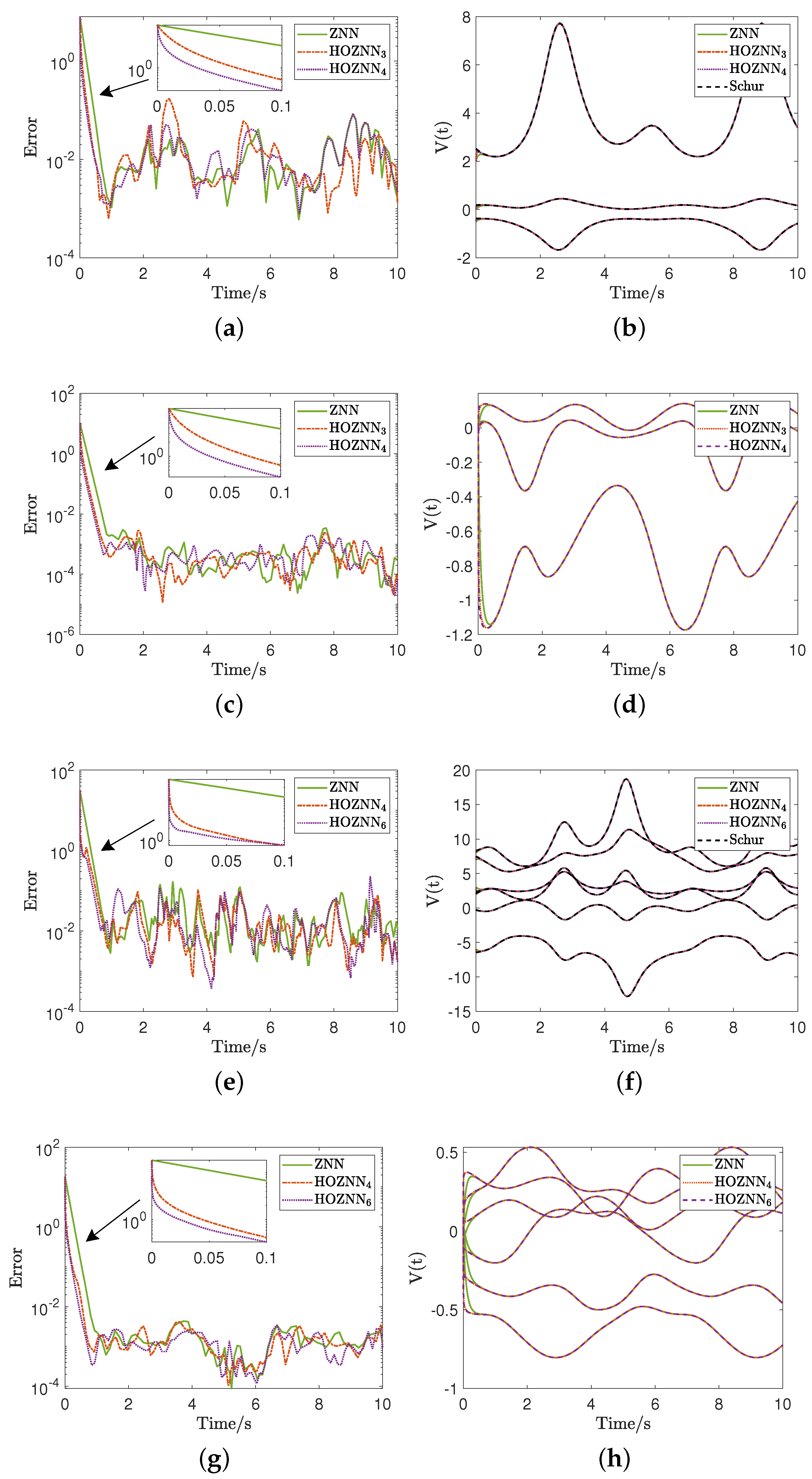
In the case of the HOZNN model, the findings are presented in Figure 1. As can be observed in Figure 1b,f, the HOZNN model yields the unique non-negative solution of the TV-ARE under IC1, which is identical to the Schur method solution. However, as can be seen in Figure 1d,h, the HOZNN model yields a random symmetric solution of the TV-ARE under IC2. This means that different symmetric TV-ARE solutions are produced from the HOZNN model for different ICs. The EME convergence of the HOZNN models is depicted in Figure 1a,c for the NE Section 4.1, and Figure 1e,g for the NE Section 4.2. In all of these figures, we observe that the EME of the HOZNN models convergence begins at $t=0$ with values in the range $[10,{10}^2]$, but it ends before $t=1$ with lowest values in the range $[{10}^{-4},{10}^{-2}]$. That is, the EME of the HOZNN models begins from a non-optimal IC and convergence to the zero matrix. Additionally, Figure 1a,c,e,g illustrate that the convergence occurs more quickly the higher the value of the parameter p. In other words, for $p=4$ the HOZNN model converges more quickly than for $p=3$, and for $p=3$, the HOZNN model converges more quickly than for $p=2$ in NE Section 4.1. Furthermore, for $p=6$, the HOZNN model converges more quickly than for $p=4$, and for $p=4$, the HOZNN model converges more quickly than for $p=2$ in NE Section 4.2. The graphs in Figure 1b,d,f,h behave in the same way due to the convergence tendency of the EME convergence of the HOZNN models. In other words, the solution trajectories associated with the HOZNN models in these figures begin at $t=0$ in a very different value from the objective and reach it before $t=1$. As a result, it is evident that Theorem 2 is proven true since we assume that $A\left(t\right),B\left(t\right),Q\left(t\right)$ are differentiable and $B\left(t\right)$, $Q\left(t\right)$ are non-negative definite and symmetric matrices.

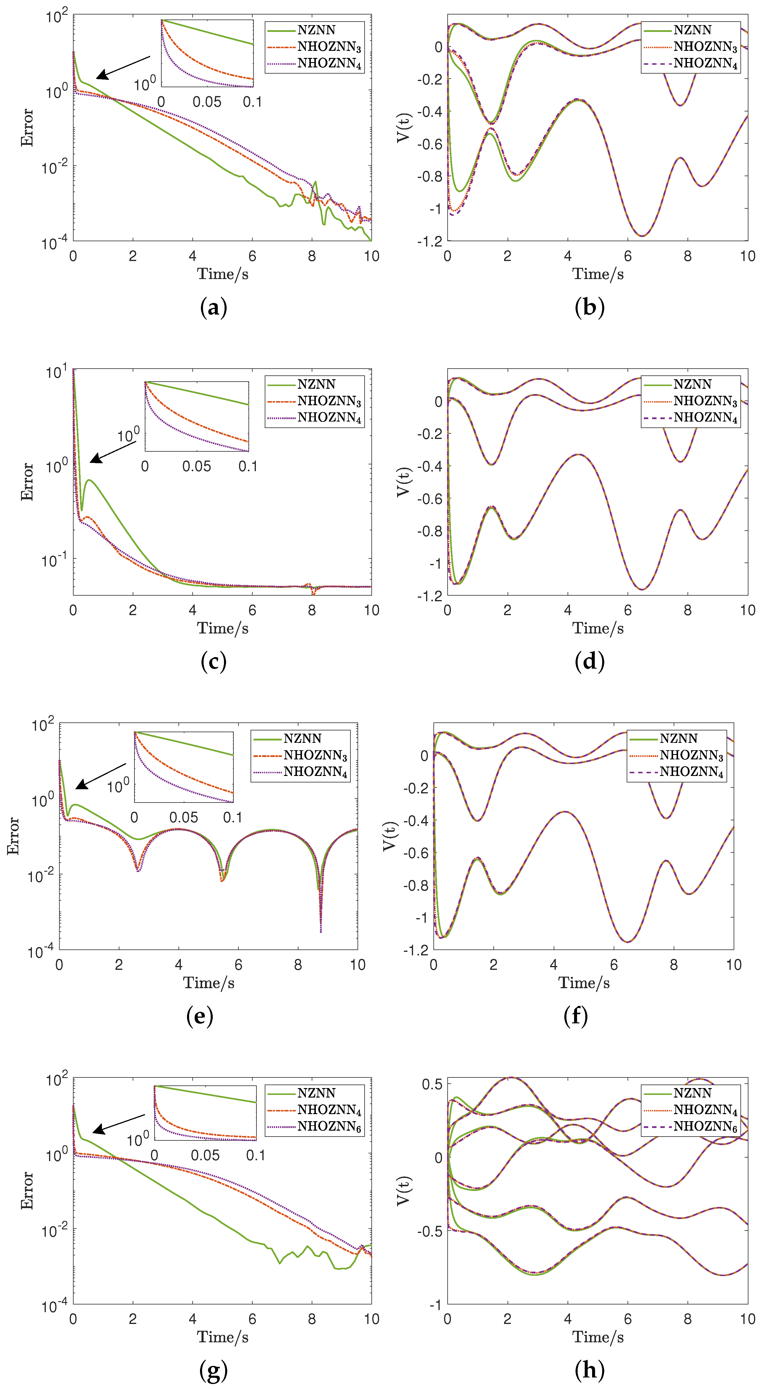
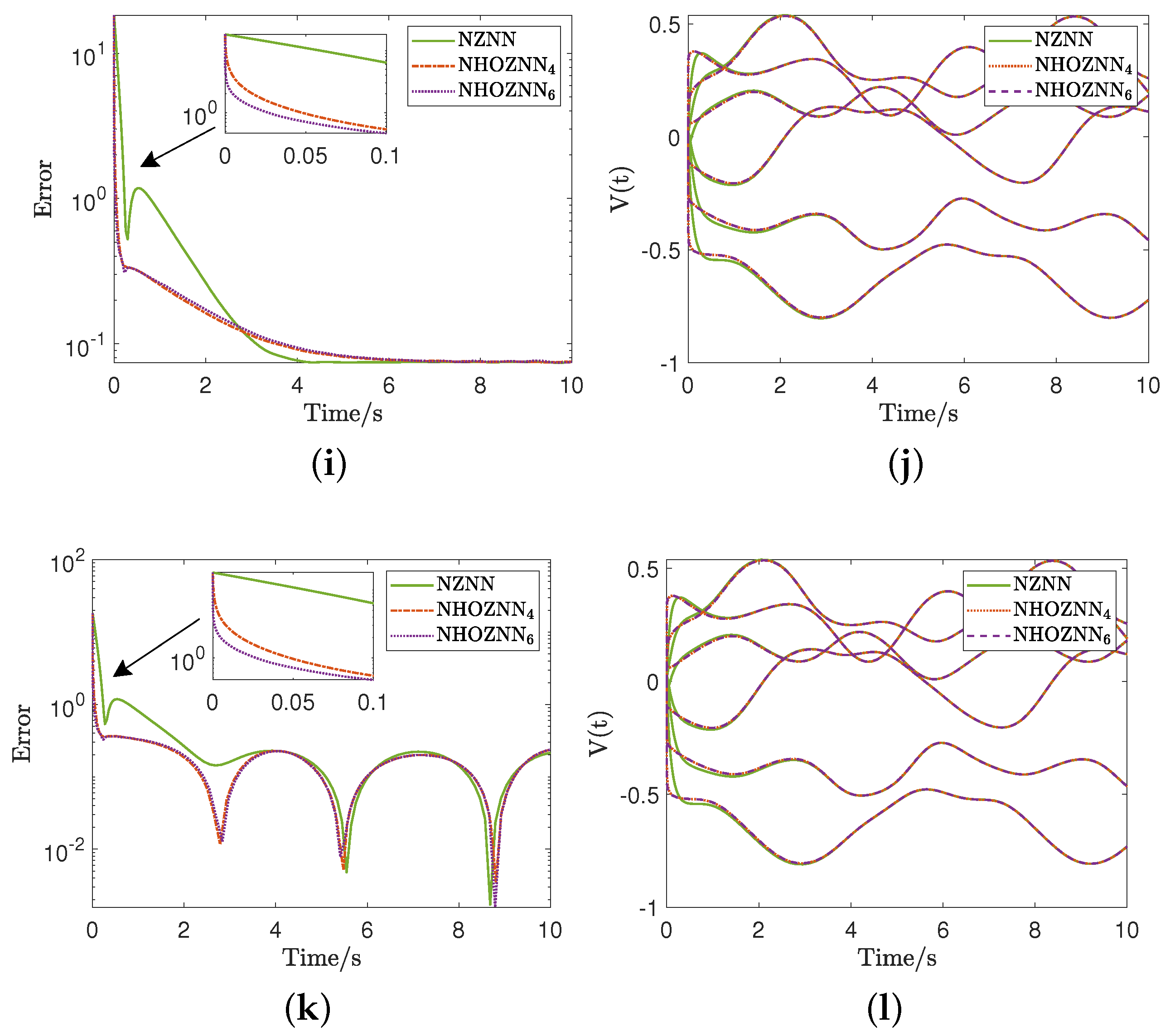
In the case of the NHOZNN model, the findings are presented in Figure 2. As can be observed in Figure 2b,d,f,h,j,l, the NHOZNN model produces a random symmetric solution to the TV-ARE of NEs Section 4.1 and Section 4.2 under IC2 with three different types of noise, CN, LN, and BRN. Further, Figure 2a,c,e,g,i,k show that for every type of noise that was utilized, the NHOZNN model converges to the TV-ARE solution. Particularly, we observe that the EME of the NHOZNN models convergence begins at $t=0$ with values in the range $[10,{10}^2]$ and, at $t=0.5$, takes values in the range $[1,{10}^{-1}]$. Until $t=10$, the EME of the NHOZNN models values continue to drop, with lowest values in the range $[{10}^{-1},{10}^{-4}]$. That is, the EME of the NHOZNN models begin from a non-optimal IC and convergence to the zero matrix. Notice also in these figures that the convergence occurs more quickly as the parameter p increases in value. The graphs in Figure 2b,d,f,h,j,l behave in the same way due to the convergence tendency of the EME convergence of the NHOZNN models under three different types of noise, CN, LN, and BRN. In other words, the solutions trajectories associated with the NHOZNN models in these figures begin at $t=0$ in a very different value from the objective and continue to drop until $t=10$ under three different types of noise. As a result, it is evident that Theorem 6 is proven true since we assume that $A\left(t\right),B\left(t\right),Q\left(t\right)$ are differentiable and $B\left(t\right)$, $Q\left(t\right)$ are non-negative definite and symmetric matrices.

The following is deduced from the NEs of this section. As the parameter p increases in value, the HOZNN and NHOZNN models perform better at solving the TV-ARE than the traditional ZNN and NZNN models, i.e., HOZNN and NHOZNN with $p=2$. In other words, the HOZNN and NHOZNN models provide the smallest Frobenius norm for the EMEs when the parameter p increases in value. It is also important to note that the models will converge more quickly the larger the value of the design parameter $\lambda$. In essence, the HOZNN and NHOZNN models outperform the traditional ZNN and NZNN models, respectively, in solving the TV-ARE.

5. Conclusions

In this paper, the problems of solving the TV-ARE is addressed by employing a family of ZNN models that correlate to the hyperpower iterative methods. As a consequence, this study proposed and examined two models: a HOZNN model that produces numerical TV-ARE real symmetric solutions, and a NHOZNN model that produces numerical TV-ARE real symmetric solutions when noise is present. The HOZNN and NHOZNN models’ exponential convergence has been demonstrated theoretically, and NEs have demonstrated that the suggested models outperform the traditional ZNN and NZNN models, respectively, at addressing the TV-ARE. Particularly, two NEs demonstrate that, beginning from non-optimal ICs, both the NHOZNN model under three distinct types of noise and the HOZNN model converge to the symmetric theoretical solutions of TV-ARE. The efficacy of the suggested models has thus been theoretically and numerically confirmed.

Some potential study topics are listed below.

• Future studies might examine the use of well chosen fuzzy parameters to create HOZNN dynamics enhancements.
• Applications in engineering [35,36,37] could demonstrate the reliability of the HOZNN dynamics in practical scenarios.

References

1. Kalman, R.E. Contributions to the theory of optimal control. Bol. Soc. Mat. Mex. 1960, 5, 102–119. [Google Scholar]
2. Qin, B.; Sun, H.; Ma, J.; Li, W.; Ding, T.; Wang, Z.; Zomaya, A.Y. Robust H control of doubly fed wind generator via state-dependent Riccati equation technique. IEEE Trans. Power Syst. 2019, 34, 2390–2400. [Google Scholar] [CrossRef]
3. Rigatos, G.; Busawon, K.; Pomares, J.; Abbaszadeh, M. Nonlinear optimal control for the wheeled inverted pendulum system. Robotica 2020, 38, 29–47. [Google Scholar] [CrossRef]
4. Dong, X.; Hu, G. Time-varying formation tracking for linear multiagent systems with multiple leaders. IEEE Trans. Autom. Control 2017, 62, 3658–3664. [Google Scholar] [CrossRef]
5. Laub, A. A Schur method for solving algebraic Riccati equations. IEEE Trans. Autom. Control 1979, 24, 913–921. [Google Scholar] [CrossRef] [Green Version]
6. Aguilar, L.T.; Orlov, Y.; Acho, L. Nonlinear H-control of nonsmooth time-varying systems with application to friction mechanical manipulators. Automatica 2003, 39, 1531–1542. [Google Scholar] [CrossRef]
7. Ferrante, A.; Ntogramatzidis, L. The generalized continuous algebraic Riccati equation and impulse-free continuous-time LQ optimal control. Automatica 2014, 50, 1176–1180. [Google Scholar] [CrossRef]
8. Ohtsuka, T. A recursive elimination method for finite-horizon optimal control problems of discrete-time rational systems. IEEE Trans. Autom. Control 2014, 59, 3081–3086. [Google Scholar] [CrossRef] [Green Version]
9. Oshman, Y.; Bar-Itzhack, I. Eigenfactor solution of the matrix Riccati equation–A continuous square root algorithm. IEEE Trans. Autom. Control 1985, 30, 971–978. [Google Scholar] [CrossRef]
10. Dooren, P.V. A generalized eigenvalue approach for solving Riccati equations. SIAM J. Sci. Stat. Comput. 1981, 2, 121–135. [Google Scholar] [CrossRef]
11. Simos, T.E.; Katsikis, V.N.; Mourtas, S.D.; Stanimirović, P.S. Finite-time convergent zeroing neural network for solving time-varying algebraic Riccati equations. J. Frankl. Inst. 2022. [Google Scholar] [CrossRef]
12. Simos, T.E.; Katsikis, V.N.; Mourtas, S.D.; Stanimirović, P.S. Unique non-negative definite solution of the time-varying algebraic Riccati equations with applications to stabilization of LTV systems. Math. Comput. Simul. 2022, 202, 164–180. [Google Scholar] [CrossRef]
13. Prach, A.; Tekinalp, O.; Bernstein, D.S. A numerical comparison of frozen-time and forward-propagating Riccati equations for stabilization of periodically time-varying systems. In Proceedings of the American Control Conference, Portland, OR, USA, 4–6 June 2014; pp. 5633–5638. [Google Scholar]
14. Prach, A.; Kayacan, E.; Bernstein, D.S. An experimental evaluation of the forward propagating Riccati equation to nonlinear control of the Quanser 3 DOF Hover testbed. In Proceedings of the 2016 American Control Conference, ACC 2016, Boston, MA, USA, 6–8 July 2016; pp. 3710–3715. [Google Scholar] [CrossRef]
15. Saiery, M.; Katebi, J.; Lakestani, M. Control of time-varying systems based on forward Riccati formulation in hybrid functions domain. Int. J. Control. 2022. [Google Scholar] [CrossRef]
16. Zhang, Y.; Ge, S.S. Design and analysis of a general recurrent neural network model for time-varying matrix inversion. IEEE Trans. Neural Netw. 2005, 16, 1477–1490. [Google Scholar] [CrossRef] [PubMed] [Green Version]
17. Jin, L.; Zhang, Y.; Li, S.; Zhang, Y. Noise-tolerant ZNN models for solving time-varying zero-finding problems: A control-theoretic approach. IEEE Trans. Autom. Control 2017, 62, 992–997. [Google Scholar] [CrossRef]
18. Jin, J.; Zhu, J.; Gong, J.; Chen, W. Novel activation functions-based ZNN models for fixed-time solving dynamirc Sylvester equation. Neural Comput. Appl. 2022, 34, 14297–14315. [Google Scholar] [CrossRef]
19. Jin, J.; Zhu, J.; Zhao, L.; Chen, L.; Chen, L.; Gong, J. A robust predefined-time convergence zeroing neural network for dynamic matrix inversion. IEEE Trans. Cybern. 2022. [Google Scholar] [CrossRef]
20. Mourtas, S.D.; Kasimis, C. Exploiting mean-variance portfolio optimization problems through zeroing neural networks. Mathematics 2022, 10, 3079. [Google Scholar] [CrossRef]
21. Kornilova, M.; Kovalnogov, V.; Fedorov, R.; Zamaleev, M.; Katsikis, V.N.; Mourtas, S.D.; Simos, T.E. Zeroing neural network for pseudoinversion of an arbitrary time-varying matrix based on singular value decomposition. Mathematics 2022, 10, 1208. [Google Scholar] [CrossRef]
22. Katsikis, V.N.; Stanimirović, P.S.; Mourtas, S.D.; Li, S.; Cao, X. Generalized Inverses: Algorithms and Applications; Mathematics Research Developments, Nova Science Publishers, Inc.: Hauppauge, NY, USA, 2021. [Google Scholar]
23. Jin, L.; Li, J.; Sun, Z.; Lu, J.; Wang, F. Neural dynamics for computing perturbed nonlinear equations applied to ACP-based lower limb motion intention recognition. IEEE Trans. Syst. Man Cybern. Syst. 2022, 52, 5105–5113. [Google Scholar] [CrossRef]
24. Jin, L.; Wei, L.; Li, S. Gradient-based differential neural-solution to time-dependent nonlinear optimization. IEEE Trans. Autom. Control. 2022. [Google Scholar] [CrossRef]
25. Climent, J.; Thome, N.; Wei, Y. A geometrical approach on generalized inverses by Neumann-type series. Linear Algebra Appl. 2001, 332, 533–540. [Google Scholar] [CrossRef] [Green Version]
26. Li, W.; Li, Z. A family of iterative methods for computing the approximate inverse of a square matrix and inner inverse of a non-square matrix. Appl. Math. Comput. 2010, 215, 3433–3442. [Google Scholar] [CrossRef]
27. Liu, X.; Jin, H.; Yu, Y. Higher-order convergent iterative method for computing the generalized inverse and its application to Toeplitz matrices. Linear Algebra Appl. 2013, 439, 1635–1650. [Google Scholar] [CrossRef]
28. Weiguo, L.; Juan, L.; Tiantian, Q. A family of iterative methods for computing Moore-Penrose inverse of a matrix. Linear Algebra Appl. 2013, 438, 47–56. [Google Scholar] [CrossRef]
29. Stanimirović, P.S.; Srivastava, S.; Gupta, D.K. From Zhang neural network to scaled hyperpower iterations. J. Comput. Appl. Math. 2018, 331, 133–155. [Google Scholar] [CrossRef]
30. Simos, T.E.; Katsikis, V.N.; Mourtas, S.D.; Stanimirović, P.S.; Gerontitis, D. A higher-order zeroing neural network for pseudoinversion of an arbitrary time-varying matrix with applications to mobile object localization. Inf. Sci. 2022, 600, 226–238. [Google Scholar] [CrossRef]
31. Stanimirović, P.S.; Katsikis, V.N.; Li, S. Higher-order ZNN dynamics. Neural Process. Lett. 2020, 51, 697–721. [Google Scholar] [CrossRef]
32. Jin, L.; Zhang, Y.; Li, S. Integration-enhanced Zhang neural network for real-time-varying matrix inversion in the presence of various kinds of noises. IEEE Trans. Neural Netw. Learn. Syst. 2016, 27, 2615–2627. [Google Scholar] [CrossRef]
33. Gupta, A.K. Numerical Methods Using MATLAB; MATLAB Solutions Series; Springer Press: New York, NY, USA, 2014. [Google Scholar]
34. Liu, H.; Wang, T.; Guo, D. Design and validation of zeroing neural network to solve time-varying algebraic Riccati equation. IEEE Access 2020, 8, 211315–211323. [Google Scholar] [CrossRef]
35. Aloui, M.; Hamidi, F.; Jerbi, H.; Omri, M.; Popescu, D.; Abbassi, R.A. Chaotic Krill Herd optimization algorithm for global numerical estimation of the attraction domain for nonlinear systems. Mathematics 2021, 9, 1743. [Google Scholar] [CrossRef]
36. Jerbi, H.; Ben Aoun, S.; Omri, M.; Simos, T.E.; Tsitouras, C. A neural network type approach for constructing Runge-Kutta pairs of orders six and five that perform best on problems with oscillatory solutions. Mathematics 2022, 10, 827. [Google Scholar] [CrossRef]
37. Jerbi, H.; Omri, M.; Kchaou, M.; Simos, T.E.; Tsitouras, C. Runge-Kutta-Nyström pairs of orders 8(6) with coefficients trained to perform best on classical orbits. Mathematics 2022, 10, 654. [Google Scholar] [CrossRef]
Figure 1. Trajectories of the HOZNN’s solutions and convergence in NEs Section 4.1 and Section 4.2 under IC1 and IC2. (a) NE Section 4.1 under IC1: convergence. (b) NE Section 4.1 under IC1: solutions trajectories. (c) NE Section 4.1 under IC2: convergence. (d) NE Section 4.1 under IC2: solutions trajectories. (e) NE Section 4.2 under IC1: convergence. (f) NE Section 4.2 under IC1: solutions trajectories. (g) NE Section 4.2 under IC2: convergence. (h) NE Section 4.2 under IC2: solutions trajectories.
Mathematics 10 04490 g001
Figure 2. Trajectories of the HOZNN’s solutions and convergence in NEs Section 4.1 and Section 4.2 with CN, LN, and BRN. (a) NE Section 4.1 with CN: convergence. (b) NE Section 4.1 with CN: solution trajectories. (c) NE Section 4.1 with LN: convergence. (d) NE Section 4.1 with LN: solution trajectories. (e) NE Section 4.1 with BRN: convergence. (f) NE Section 4.1 with BRN: solution trajectories. (g) NE Section 4.2 with CN: convergence. (h) NE Section 4.2 with CN: solution trajectories. (i) NE Section 4.2 with LN: convergence. (j) NE Section 4.2 with LN: solution trajectories. (k) NE Section 4.2 with BRN: convergence. (l) NE Section 4.2 with BRN: solution trajectories.
Mathematics 10 04490 g002aMathematics 10 04490 g002b
Publisher’s Note: MDPI stays neutral with regard to jurisdictional claims in published maps and institutional affiliations.