A Convergent Algorithm for Equilibrium Problem to Predict Prospective Mathematics Teachers’ Technology Integrated Competency

Abstract

Educational data classification has become an effective tool for exploring the hidden pattern or relationship in educational data and predicting students’ performance or teachers’ competency. This study proposes a new method based on machine learning algorithms to predict the technology-integrated competency of pre-service mathematics teachers. In this paper, we modified the inertial subgradient extragradient algorithm for pseudomonotone equilibrium and proved the weak convergence theorem under some suitable conditions in Hilbert spaces. We then applied to solve data classification by extreme learning machine using the dataset comprised of the technology-integrated competency of 954 pre-service mathematics teachers in a university in northern Thailand, longitudinally collected for five years. The flexibility of our algorithm was shown by comparisons of the choice of different parameters. The performance was calculated and compared with the existing algorithms to be implemented for prediction. The results show that the proposed method achieved a classification accuracy of 81.06%. The predictions were implemented using ten attributes, including demographic information, skills, and knowledge relating to technology developed throughout the teacher education program. Such data driven studies are significant for establishing a prospective teacher competency analysis framework in teacher education and contributing to decision-making for policy design.

1. Introduction

The National Council of Teachers of Mathematics (NCTM) [1] reports that teaching with technology to support conceptual development has been a focus of mathematics education for decades. Utilizing multiple technologies to teach mathematics is significantly more difficult than using technology in everyday life. It included teachers’ perspectives, recognizing the significance of technology in teaching mathematics and their confidence in using technology when constructing relevant technology-integrated mathematics classrooms. Therefore, the technology-integrated competency of teachers was defined in this study as the competency to design mathematics lessons that enable students to work on challenging mathematics problems through technology [2,3,4,5].

To unleash the benefits of technology in the mathematics classroom [6,7], teachers require extensive preparation and support. Accordingly, the integration of technology in mathematics education to produce competent prospective mathematics teachers has been incorporated into the most recent mathematics teacher preparation standards [8]. Utilizing validated classification to evaluate prospective mathematics teachers’ technology-integrated competency provides a solid foundation for entry into the profession [9,10].

In recent years, there has been significant interest in the application of data classification approaches to the field of education. Classification is a method for identifying the class of data points provided, referred to as targets/labels or categories. It can be the study of discovering new and potentially helpful information or meaningful outcomes from data. It also seeks to obtain new trends and patterns from datasets by employing various categorization techniques. Particularly, data classification in the education field is now an effective technique for identifying hidden patterns in educational data, predicting students’ academic performance, determining teachers’ competency or enhancing the learning and teaching policy plan. Thus, in this study, we focused on prospective mathematics teachers’ information as our educational data, longitudinally collected over five years, for classification to identify hidden patterns in their technology-integrated competency development.

First of all, we studied the equilibrium problem (EP), initially introduced by Muu and Oettli [11]. The EP is to find an element $z^{*}$ in a nonempty closed convex subset C of a real Hilbert space $\mathcal{H}$ such that

$$f(z^{*},y)\ge 0,\forall y\in C,$$

(1)

where $f:\mathcal{H}\times \mathcal{H}\to \mathbb{R}$ is a bifunction with $f(x,x)=0$ for all $x\in C$, and $EP(C,f)$ is denoted for a solution set of the EP (1). The EP (1) generalizes various mathematical problems in optimization analysis such as variational inequalities, minimization problems, linear programming problems, and Nash equilibrium problems, among others, see in [12,13,14,15].

In 2008, Tran et al. [16] presented the two-step extragradient method (TSEM) for solving the EP (1), which is inspired by the concept of solving the variational inequalities of Korpelevich [17]. The iterative scheme is formulated as follows: $x_1\in C$ and

$$\begin{array}{ll}{y}_n& =arg\underset{y\in C}{min}\left\{\lambda f(x_n,y)+\frac{1}{2}{\parallel x_n-y\parallel }^2\right\},\\ x_{n+1}\hfill & =arg\underset{y\in C}{min}\left\{\lambda f(y_n,y)+\frac{1}{2}{\parallel x_n-y\parallel }^2\right\},\hfill \end{array}$$

(2)

where $\lambda$ is some constant depending on the interval that makes the bifunction f satisfy the Lipschitz condition. However, as remarked by the authors of [18], two projections on C of the two-step extragradient algorithm, which was introduced by Korpelevich [17], are very difficult to use and can affect the efficiency of the method if C has a complex structure.

In 2019, Rehman et al. [19] modified the subgradient explicit iterative algorithm to solve the problem of pseudomonotone equilibrium problems. The weak convergence of these algorithms is well established under stepsize, which are updated at each iteration without the Lipschitz-type condition. The algorithm is generated by arbitrary elements $x_0\in \mathcal{H}$, ${\lambda }_0>0$ and $\mu \in (0,1)$,

$$\begin{array}{cc}{y}_n\hfill & =arg\underset{y\in C}{min}\left\{{\lambda }_{n}f(x_n,y)+\frac{1}{2}{\parallel x_n-y\parallel }^2\right\},\hfill \\ x_{n+1}\hfill & =arg\underset{y\in {\mathcal{H}}_n}{min}\left\{{\lambda }_{n}f(y_n,y)+\frac{1}{2}{\parallel x_n-y\parallel }^2\right\},\hfill \end{array}$$

(3)

where $w_n\in {\partial }_{2}f(x_n,y_n)$ satisfy $x_n-{\lambda }_n{w}_n-y_n\in N_C\left(y_n\right)$ with a half-space

$${\mathcal{H}}_n=\{z\in \mathcal{H}:\langle x_n-{\lambda }_n{w}_n-y_n,z-y_n\rangle \le 0\},$$

and

$${\lambda }_{n+1}=\left\{{\lambda }_n,\frac{\mu \left(\parallel x_n-y_n{\parallel }^2+{\parallel x_{n+1}-y_n\parallel }^2\right)}{2[f(x_n,x_{n+1})-f(x_n,y_n)-f(y_n,x_{n+1})]}\right\}.$$

Very recently, Rehman et al. [20] focused on improving the stepsize of the subgradient extragradient method to find a solution to the problems of pseudo-monotone equilibrium in a real Hilbert space. The inertial technique term which was first proposed by Polyak [21] was added to speed up the convergence of the algorithm. The weak convergence of the method is well-established based on the standard assumptions on a bifunction. This algorithm is generated by arbitrary elements $x_0,x_1\in \mathcal{H}$. Choose $\varrho \in (0,1)$, $\sigma <min\left\{\frac{1-3\delta }{{(1-\delta )}^2},\frac{1}{2c_1},\frac{1}{2c_2}\right\}$, $\mu \in (0,\sigma )$, ${\lambda }_1>0$ and non-decreasing sequence $0\le {\delta }_n\le \delta \in [0,\frac{1}{3})$;

$$\begin{array}{cc}{\rho }_n\hfill & =x_n+{\delta }_n(x_n-x_{n-1})\hfill \\ y_n\hfill & =arg\underset{y\in C}{min}\left\{{\lambda }_{n}f({\rho }_n,y)+\frac{1}{2}{\parallel {\rho }_n-y\parallel }^2\right\},\hfill \\ x_{n+1}\hfill & =arg\underset{y\in {\mathcal{H}}_n}{min}\left\{{\lambda }_{n}f(y_n,y)+\frac{1}{2}{\parallel {\rho }_n-y\parallel }^2\right\},\hfill \end{array}$$

(4)

where $w_n\in {\partial }_{2}f({\rho }_n,y_n)$ satisfy ${\rho }_n-{\lambda }_n{w}_n-y_n\in N_C\left(y_n\right)$ and construct a half-space

$${\mathcal{H}}_n=\{z\in \mathcal{H}:\langle {\rho }_n-{\lambda }_n{w}_n-y_n,z-y_n\rangle \le 0\},$$

and

$${\lambda }_{n+1}=\left\{\sigma ,\frac{\mu f(y_n,x_{n+1})}{f({\rho }_n,x_{n+1})-f({\rho }_n,y_n)-c_1\parallel {\rho }_n-y_n{\parallel }^2-c_2{\parallel x_{n+1}-y_n\parallel }^2+1}\right\}.$$

Inspired by the above research, we introduce a new modified inertial subgradient extragradient method for obtaining weak convergence to a solution of the set $EP(f,C)$ and try to relax the update stepsize $\left\{{\lambda }_n\right\}$ that can be chosen in many ways. In applications, we apply our algorithm to solve classification problems in machine learning and show the performance of our algorithm by comparing it with existing algorithms to predict prospective mathematics teachers’ technology-integrated competency.

2. Preliminaries

In what follows, recall that $\mathcal{H}$ is a real Hilbert space. Let C be a nonempty, closed and convex subset of $\mathcal{H}$. We denote ⇀ and → as weak and strong convergence, respectively. We next collect some necessary definitions and lemmas for proving our main results. Assume $u,v\in \mathcal{H}$,

$$\begin{array}{cc}{\parallel au+(1-a)v\parallel }^2\hfill & ={a\parallel u\parallel }^2+{(1-a)\parallel v\parallel }^2-a(1-a){\parallel u-v\parallel }^2\hfill \end{array}$$

(5)

for any $a\in [0,1]$.

A normal cone of C at $x\in C$ is defined by

$$N_C\left(x\right)=\{z\in \mathcal{H}:\langle z,y-x\rangle \le 0,\mathrm{for}\mathrm{all}y\in C\}.$$

Let $g:C\to \mathbb{R}$ be a convex function and subdifferential of g at $x\in C$ defined by

$$\partial g\left(x\right)=\{z\in \mathcal{H}:g(y)-g(x)\ge \langle z,y-x\rangle ,\mathrm{for}\mathrm{all}y\in C\}.$$

A bifunction $f:\mathcal{H}\times \mathcal{H}\to \mathbb{R}$ on C is stated to be

$\left(i\right)$ pseudomonotone if $f(u,v)\ge 0⟹f(v,u)\le 0,\mathrm{for}\mathrm{all}u,v\in C$;

$\left(ii\right)$ satisfies the Lipschitz-like criteria for some $c_1,c_2>0$, the following inequality is satisfied

$$f(u,w)\le f(u,v)+f(v,w)+c_1{\parallel u-v\parallel }^2+c_2{\parallel v-w\parallel }^2,\mathrm{for}\mathrm{all}u,v,w\in C.$$

Lemma 1

([22]). Let $g:C\to \mathbb{R}$ be a subdifferentiable, convex and lower semi-continuous function on C. An element $x\in C$ is a minimizer of a function g if and only if

$$0\in \partial g\left(x\right)+N_C\left(x\right),$$

where $\partial g\left(x\right)$ stands for the subdifferential of g at $x\in C$ and $N_C\left(x\right)$ the normal cone of C at x.

Lemma 2

([23]). Let $\left\{a_n\right\}$ and $\left\{b_n\right\}$ be nonnegative sequences of real numbers satisfying ${\displaystyle \sum _{n=1}^{\infty }{b}_n<\infty }$ and $a_{n+1}\le a_n+b_n.$ Then, $\left\{a_n\right\}$ is a convergent sequence.

Lemma 3

([24], Opial). Let Φ be a nonempty set of $\mathcal{H}$ and $\left\{x_n\right\}$ be a sequence in $\mathcal{H}$. Suppose the following assertions hold.

$\left(i\right)$ For every $x\in \Phi$, the sequence $\left\{\parallel x_n-x\parallel \right\}$ converges;

$\left(ii\right)$ Every weak sequential cluster point of $\left\{x_n\right\}$ belongs to Φ.

Then $\left\{x_n\right\}$ converges weakly to a point in Φ.

3. Convergence Theorem

To study the convergence analysis, consider the following conditions.

$\left(\mathcal{C}1\right)$ The solution set $EP(f,C)$ is nonempty and f is pseudomonotone on C;

$\left(\mathcal{C}2\right)$f meets the Lipschitz-like condition on $\mathcal{H}$ through $c_1>0$ and $c_2>0$;

$\left(\mathcal{C}3\right)$$f(z,·)$ is subdifferentiable and convex on $\mathcal{H}$ for each fixed $z\in \mathcal{H}$;

$\left(\mathcal{C}4\right)$${\displaystyle \underset{n\to \infty }{lim\; sup}f(z_n,y)\le f(z^{*},y)}$ for each $y\in C$ and $\left\{z_n\right\}\subset C$ satisfies $z_n\rightharpoonup z^{*}$.

Lemma 4.

Let ${\rho }_n=y_n$ in Algorithm 1, then ${\rho }_n\in EP(f,C)$.

Algorithm 1 Modified inertial subgradient extragradient Mann Algorithm 1

Initialization: Select arbitrary elements $x_0,x_1\in \mathcal{H}$. Iterative Steps: Construct $\left\{x_n\right\}$ by using the following steps: Step 1. Set ${\rho }_n=x_n+{\delta }_n(x_n-x_{n-1})$, where $\left\{{\delta }_n\right\}\subset [0,\infty )$, and compute $$\begin{array}{cc}{y}_n\hfill & =arg\underset{y\in C}{min}\left\{{\lambda }_{n}f({\rho }_n,y)+\frac{1}{2}{\parallel {\rho }_n-y\parallel }^2\right\},\hfill \end{array}$$ where $0<{\lambda }_n\le \lambda <min\left\{\frac{1}{2c_1},\frac{1}{2c_2}\right\}$. If ${\rho }_n=y_n$, then stop. Otherwise, Step 2. Compute $$\begin{array}{cc}{u}_n\hfill & =arg\underset{y\in {\mathcal{H}}_n}{min}\left\{{\lambda }_{n}f(y_n,y)+\frac{1}{2}{\parallel {\rho }_n-y\parallel }^2\right\},\hfill \end{array}$$ where $w_n\in {\partial }_{2}f({\rho }_n,y_n)$ satisfying ${\rho }_n-{\lambda }_n{w}_n-y_n\in N_C\left(y_n\right)$ and construct a half-space $$\begin{array}{cc}{\mathcal{H}}_n\hfill & =\{z\in \mathcal{H}:\langle {\rho }_n-{\lambda }_n{w}_n-y_n,z-y_n\rangle \le 0\}.\hfill \end{array}$$ Step 3. Compute $$\begin{array}{cc}{x}_{n+1}\hfill & ={\theta }_n{\rho }_n+(1-{\theta }_n)u_n,\hfill \end{array}$$ where $\left\{{\theta }_n\right\}\subset (0,1)$. Replace n with $n+1$ and then repeat Step 1.

Proof. 

By the definition of $y_n$ with Lemma 1, we have

$$\begin{array}{c}0\in {\partial }_2\left({\lambda }_{n}f({\rho }_n,·)+\frac{1}{2}{\parallel {\rho }_n-·\parallel }^2\right)\left(y_n\right)+N_C\left(y_n\right).\hfill \end{array}$$

Thus, we can write ${\lambda }_n{\tilde{w}}_n+y_n-{\rho }_n+{\overline{w}}_n=0$, where ${\tilde{w}}_n\in {\partial }_{2}f({\rho }_n,y_n)$ and ${\overline{w}}_n\in N_C\left(y_n\right)$. Due to ${\rho }_n=y_n$ implies that ${\lambda }_n{\tilde{w}}_n+{\overline{w}}_n=0$. Thus, we have

$$\begin{array}{c}{\lambda }_n\langle {\tilde{w}}_n,y-y_n\rangle +\langle {\overline{w}}_n,y-y_n\rangle =0\hfill \end{array}$$

for all $y\in C$. By ${\overline{w}}_n\in N_C\left(y_n\right)$ implies $\langle {\overline{w}}_n,y-y_n\rangle \le 0$ for all $y\in C$ and through above expression, we obtain

$$\begin{array}{c}{\lambda }_n\langle {\tilde{w}}_n,y-y_n\rangle \ge 0\hfill \end{array}$$

(6)

for all $y\in C$. Due to ${\tilde{w}}_n\in {\partial }_{2}f({\rho }_n,y_n)$ and using the subdifferential definition, we obtain

$$\begin{array}{c}\langle {\tilde{w}}_n,y-y_n\rangle \le f({\rho }_n,y)-f({\rho }_n,y_n)\hfill \end{array}$$

(7)

for all $y\in C$. From the inequalities (6) and (7) with $0<{\lambda }_n\le \lambda$ implies that $f({\rho }_n,y)\ge 0$ for all $y\in C$, that is, ${\rho }_n\in EP(f,C)$.    □

Lemma 5.

Suppose that $f:\mathcal{H}\times \mathcal{H}\to \mathbb{R}$ meet the items $\left(\mathcal{C}1\right)-\left(\mathcal{C}3\right)$, we have

$$\begin{array}{c}\parallel u_n-\overline{\xi }{\parallel }^2+(1-2c_1{\lambda }_n)\parallel {\rho }_n-y_n{\parallel }^2+(1-2c_2{\lambda }_n)\parallel y_n-u_n{\parallel }^2\le {\parallel {\rho }_n-\overline{\xi }\parallel }^2\hfill \end{array}$$

(8)

for all $\overline{\xi }\in EP(f,C)$.

Proof. 

Let $\overline{\xi }\in EP(f,C)$, then by using Lemma 1, we have

$$\begin{array}{c}0\in {\partial }_2\left({\lambda }_{n}f(y_n,·)+\frac{1}{2}{\parallel {\rho }_n-·\parallel }^2\right)\left(u_n\right)+N_{{\mathcal{H}}_n}\left(u_n\right).\hfill \end{array}$$

Thus, we can write ${\lambda }_n{\tilde{w}}_n+u_n-{\rho }_n+{\overline{w}}_n=0$, where ${\tilde{w}}_n\in {\partial }_{2}f(y_n,u_n)$ and ${\overline{w}}_n\in N_{{\mathcal{H}}_n}\left(u_n\right)$. This implies that

$$\begin{array}{c}\langle {\rho }_n-u_n,y-u_n\rangle ={\lambda }_n\langle {\tilde{w}}_n,y-u_n\rangle +\langle {\overline{w}}_n,y-u_n\rangle \hfill \end{array}$$

for all $y\in {\mathcal{H}}_n$. Given that ${\overline{w}}_n\in N_{{\mathcal{H}}_n}\left(u_n\right)$ then $\langle {\overline{w}}_n,y-u_n\rangle \le 0$ for all $y\in {\mathcal{H}}_n$. Therefore, we have

$$\begin{array}{c}\langle {\rho }_n-u_n,y-u_n\rangle \le {\lambda }_n\langle {\tilde{w}}_n,y-u_n\rangle \hfill \end{array}$$

(9)

for all $y\in {\mathcal{H}}_n$. Since ${\tilde{w}}_n\in {\partial }_{2}f(y_n,u_n)$, we have

$$\begin{array}{c}\langle {\tilde{w}}_n,y-u_n\rangle \le f(y_n,y)-f(y_n,u_n)\hfill \end{array}$$

(10)

for all $y\in \mathcal{H}$. From (9) and (10), we obtain

$$\begin{array}{c}\langle {\rho }_n-u_n,y-u_n\rangle \le {\lambda }_{n}f(y_n,y)-{\lambda }_{n}f(y_n,u_n)\hfill \end{array}$$

(11)

for all $y\in {\mathcal{H}}_n$. Substituting $y=\overline{\xi }$ in (9), we obtain

$$\begin{array}{c}\langle {\rho }_n-u_n,\overline{\xi }-u_n\rangle \le {\lambda }_{n}f(y_n,\overline{\xi })-{\lambda }_{n}f(y_n,u_n).\hfill \end{array}$$

(12)

Given $\overline{\xi }\in EP(f,C)$ imply that $f(\overline{\xi },y_n)\ge 0$ and owing to the item $\left(\mathcal{C}1\right)$ gives that $f(y_n,\overline{\xi })\le 0$. Thus, we obtain

$$\begin{array}{c}\langle {\rho }_n-u_n,u_n-\overline{\xi }\rangle \ge {\lambda }_{n}f(y_n,u_n).\hfill \end{array}$$

(13)

Following the condition $\left(\mathcal{C}2\right)$, we have

$$\begin{array}{c}f(y_n,u_n)\ge f({\rho }_n,u_n)-f({\rho }_n,y_n)-c_1\parallel {\rho }_n-y_n{\parallel }^2-c_2{\parallel y_n-u_n\parallel }^2.\hfill \end{array}$$

(14)

Combining (13) and (14), we obtain

$$\begin{array}{c}\langle {\rho }_n-u_n,u_n-\overline{\xi }\rangle \ge {\lambda }_{n}f({\rho }_n,u_n)-{\lambda }_{n}f({\rho }_n,y_n)-c_1{\lambda }_n\parallel {\rho }_n-y_n{\parallel }^2-c_2{\lambda }_n{\parallel y_n-u_n\parallel }^2.\hfill \end{array}$$

(15)

By using the half-space definition, we have $\langle {\rho }_n-{\lambda }_n{w}_n-y_n,u_n-y_n\rangle \le 0$, which implies that

$$\begin{array}{c}\langle {\rho }_n-y_n,u_n-y_n\rangle \le {\lambda }_n\langle w_n,u_n-y_n\rangle .\hfill \end{array}$$

(16)

Since $w_n\in {\partial }_{2}f({\rho }_n,y_n)$, we obtain

$$\begin{array}{c}\langle w_n,y-y_n\rangle \le f({\rho }_n,y)-f({\rho }_n,y_n)\hfill \end{array}$$

for all $y\in \mathcal{H}$. By replacing $y=u_n$, we obtain

$$\begin{array}{c}\langle w_n,u_n-y_n\rangle \le f({\rho }_n,u_n)-f({\rho }_n,y_n).\hfill \end{array}$$

(17)

It follows from inequalities (16) and (17) that

$$\begin{array}{c}\langle {\rho }_n-y_n,u_n-y_n\rangle \le {\lambda }_{n}f({\rho }_n,u_n)-{\lambda }_{n}f({\rho }_n,y_n).\hfill \end{array}$$

(18)

From (15) and (18), we have

$$\begin{array}{c}\langle {\rho }_n-u_n,u_n-\overline{\xi }\rangle \ge \langle {\rho }_n-y_n,u_n-y_n\rangle -c_1{\lambda }_n\parallel {\rho }_n-y_n{\parallel }^2-c_2{\lambda }_n{\parallel y_n-u_n\parallel }^2.\hfill \end{array}$$

(19)

Now, we obtain the following equalities:

$$\begin{array}{c}\parallel {\rho }_n-\overline{\xi }{\parallel }^2-\parallel u_n-{\rho }_n{\parallel }^2-{\parallel u_n-\overline{\xi }\parallel }^2=2\langle {\rho }_n-u_n,u_n-\overline{\xi }\rangle \hfill \end{array}$$

and

$$\begin{array}{c}\parallel {\rho }_n-y_n{\parallel }^2+\parallel u_n-y_n{\parallel }^2-{\parallel {\rho }_n-u_n\parallel }^2=2\langle {\rho }_n-y_n,u_n-y_n\rangle .\hfill \end{array}$$

Combining the above equalities with expression (19) finalizes the proof.    □

Lemma 6.

Assume that the items $\left(\mathcal{C}1\right)-\left(\mathcal{C}4\right)$ hold. If there is a subsequence $\left\{{\rho }_{n_k}\right\}$ of $\left\{{\rho }_n\right\}$ such that ${\rho }_{n_k}\rightharpoonup x^{*}\in \mathcal{H}$ and

$$\begin{array}{c}\underset{k\to \infty }{lim}\parallel {\rho }_{n_k}-y_{n_k}\parallel =\underset{k\to \infty }{lim}\parallel {\rho }_{n_k}-u_{n_k}\parallel =\underset{k\to \infty }{lim}\parallel u_{n_k}-y_{n_k}\parallel =0,\hfill \end{array}$$

(20)

then $x^{*}\in EP(f,C)$.

Proof. 

From $y_n\in C$, ${\rho }_{n_k}\rightharpoonup x^{*}$ and ${\displaystyle \underset{k\to \infty }{lim}\parallel {\rho }_{n_k}-y_{n_k}\parallel =0}$, we get $y_{n_k}\rightharpoonup x^{*}\in C$. This follows from ${\displaystyle \underset{k\to \infty }{lim}\parallel u_{n_k}-y_{n_k}\parallel =0}$ that the subsequence $\left\{u_{n_k}\right\}$ is bounded. For any $y\in {\mathcal{H}}_n$, using (11), (14) and (18), we have

$$\begin{array}{cc}{\lambda }_{n_k}f(y_{n_k},y)\hfill & \ge {\lambda }_{n_k}f(y_{n_k},u_{n_k})+\langle {\rho }_{n_k}-u_{n_k},y-u_{n_k}\rangle \hfill \\ \hfill & \ge {\lambda }_{n_k}f({\rho }_{n_k},u_{n_k})-{\lambda }_{n_k}f({\rho }_{n_k},y_{n_k})-c_1{\lambda }_{n_k}\parallel {\rho }_{n_k}-y_{n_k}{\parallel }^2-c_2{\lambda }_{n_k}{\parallel y_{n_k}-u_{n_k}\parallel }^2\hfill \\ \hfill & +\langle {\rho }_{n_k}-u_{n_k},y-u_{n_k}\rangle \hfill \\ \hfill & \ge \langle {\rho }_{n_k}-y_{n_k},u_{n_k}-y_{n_k}\rangle +\langle {\rho }_{n_k}-u_{n_k},y-u_{n_k}\rangle -c_1{\lambda }_{n_k}{\parallel {\rho }_{n_k}-y_{n_k}\parallel }^2\hfill \\ \hfill & -c_2{\lambda }_{n_k}{\parallel y_{n_k}-u_{n_k}\parallel }^2.\hfill \end{array}$$

This implies by (20) and the boundedness of $\left\{u_{n_k}\right\}$ that the right hand side tends to zero. Due to $0<{\lambda }_{n_k}\le \lambda <min\left\{\frac{1}{2c_1},\frac{1}{2c_2}\right\}$, the condition $\left(\mathcal{C}4\right)$, and $y_{n_k}\rightharpoonup x^{*}$, we obtain ${\displaystyle 0 \le \underset{k\to \infty }{lim\; sup}f(y_{n_k},y)\le f(x^{*},y)}$ for all $y\in {\mathcal{H}}_n$. Since $C\subset {\mathcal{H}}_n$, we get $f(x^{*},y)\ge 0$ for all $y\in C$, that is, $x^{*}\in EP(f,C)$.    □

With the above results, we are now ready for the main convergence theorem.

Theorem 1.

Suppose that ${\displaystyle \sum _{n=1}^{\infty }{\delta }_n\parallel x_n-x_{n-1}\parallel <\infty ,\underset{n\to \infty }{lim\; inf}{\theta }_n(1-{\theta }_n)>0}$ and the items $\left(\mathcal{C}1\right)-\left(\mathcal{C}4\right)$ are satisfied. Then, the sequence $\left\{x_n\right\}$ generated due to Algorithm 1 converges weakly to a point in $EP(f,C)$.

Proof. 

Let $\overline{\xi }\in EP(f,C)$. Since $0<{\lambda }_n\le \lambda <min\left\{\frac{1}{2c_1},\frac{1}{2c_2}\right\}$ with expression (8) implies that

$$\begin{array}{c}\parallel u_n-\overline{\xi }\parallel \le \parallel {\rho }_n-\overline{\xi }\parallel .\hfill \end{array}$$

(21)

By the definition of ${\rho }_n$ and ${\displaystyle \sum _{n=1}^{\infty }{\delta }_n\parallel x_n-x_{n-1}\parallel <\infty }$, we get

$$\begin{array}{c}\underset{n\to \infty }{lim}\parallel {\rho }_n-x_n\parallel =\underset{n\to \infty }{lim}{\delta }_n\parallel x_n-x_{n-1}\parallel =0.\hfill \end{array}$$

(22)

Next, from the definitions of ${\rho }_n$ and $x_{n+1}$, and using (21), the following relation is obtained:

$$\begin{array}{cc}\parallel x_{n+1}-\overline{\xi }\parallel \hfill & \le {\theta }_n\parallel {\rho }_n-\overline{\xi }\parallel + (1-{\theta }_n)\parallel u_n-\overline{\xi }\parallel \hfill \\ \hfill & \le {\theta }_n\parallel {\rho }_n-\overline{\xi }\parallel + (1-{\theta }_n)\parallel {\rho }_n-\overline{\xi }\parallel \hfill \\ \hfill & =\parallel {\rho }_n-\overline{\xi }\parallel \hfill \\ \hfill & \le \parallel x_n-\overline{\xi }\parallel + {\delta }_n\parallel x_n-x_{n-1}\parallel .\hfill \end{array}$$

(23)

Applying this to ${\displaystyle \sum _{n=1}^{\infty }{\delta }_n\parallel x_n-x_{n-1}\parallel <\infty }$ with Lemma 2, we can conclude that the sequence $\left\{\parallel x_n-\overline{\xi }\parallel \right\}$ converges. It follows from (22) and (23) that

$$\begin{array}{c}\underset{n\to \infty }{lim}\parallel x_n-\overline{\xi }\parallel = \underset{n\to \infty }{lim}\parallel {\rho }_n-\overline{\xi }\parallel .\hfill \end{array}$$

(24)

Next, applying the definition of $x_{n+1}$ with (5) and (21), we have

$$\begin{array}{cc}\parallel x_{n+1}-\overline{\xi }{\parallel }^2\hfill & \le {\theta }_n\parallel {\rho }_n-\overline{\xi }{\parallel }^2+(1-{\theta }_n)\parallel u_n-\overline{\xi }{\parallel }^2-{\theta }_n(1-{\theta }_n){\parallel {\rho }_n-u_n\parallel }^2\hfill \\ \hfill & \le \parallel {\rho }_n-\overline{\xi }{\parallel }^2-{\theta }_n(1-{\theta }_n){\parallel {\rho }_n-u_n\parallel }^2,\hfill \end{array}$$

which means that

$$\begin{array}{cc}{\theta }_n(1-{\theta }_n){\parallel {\rho }_n-u_n\parallel }^2\hfill & \le \parallel {\rho }_n-\overline{\xi }{\parallel }^2-{\parallel x_{n+1}-\overline{\xi }\parallel }^2.\hfill \end{array}$$

It is implied by expression (24) and ${\displaystyle \underset{n\to \infty }{lim\; inf}{\theta }_n(1-{\theta }_n)>0}$ that

$$\begin{array}{c}\underset{n\to \infty }{lim}\parallel {\rho }_n-u_n\parallel =0.\hfill \end{array}$$

(25)

By the inequality (8), we obtain

$$\begin{array}{cc}(1-2c_1{\lambda }_n)\parallel {\rho }_n-y_n{\parallel }^2+(1-2c_2{\lambda }_n){\parallel y_n-u_n\parallel }^2\hfill & \le \parallel {\rho }_n-\overline{\xi }{\parallel }^2 - {\parallel u_n-\overline{\xi }\parallel }^2\hfill \\ \hfill & \le \left(\parallel {\rho }_n-\overline{\xi }\parallel + \parallel u_n-\overline{\xi }\parallel \right)\left(\parallel {\rho }_n-\overline{\xi }\parallel - \parallel u_n-\overline{\xi }\parallel \right)\hfill \\ \hfill & \le \overline{M}\parallel {\rho }_n-u_n\parallel \hfill \end{array}$$

(26)

for some $\overline{M}>0$. Using (25) with (26) and $0<{\lambda }_n\le \lambda <min\left\{\frac{1}{2c_1},\frac{1}{2c_2}\right\}$, we infer that

$$\begin{array}{c}\underset{n\to \infty }{lim}\parallel {\rho }_n-y_n\parallel =\underset{n\to \infty }{lim}\parallel y_n-u_n\parallel =0.\hfill \end{array}$$

(27)

Finally, let $x^{*}\in \mathcal{H}$ such that $x_{n_k}\rightharpoonup x^{*}$ as $k\to \infty$ for some subsequence $\left\{x_{n_k}\right\}$ of $\left\{x_n\right\}$. By (22), we get ${\rho }_{n_k}\rightharpoonup x^{*}$ as $k\to \infty$. Then, Lemma 6 together with (25) and (27) implies that $x^{*}\in EP(f,C)$. Using Opial’s lemma (Lemma 3), we can conclude that $\left\{x_n\right\}$ converges weakly to a point in $EP(f,C)$.    □

We next show that we can construct stepsizes under the Lipschitz-like condition of the parameter ${\lambda }_n$ for obtaining new algorithms in many ways. This means that our algorithm is flexible to use. Inspired by the stepsize idea of Rehman et al. [19,20], we can modify stepsizes $\left\{{\lambda }_n\right\}$ for our Algorithm 1 which satisfy the condition that $0<{\lambda }_n\le \lambda <min\left\{\frac{1}{2c_1},\frac{1}{2c_2}\right\}$; then, we obtain the following algorithms.

4. Application to Data Classification Problem of Educational Dataset

The educational dataset shown in this classification is prospective mathematics teachers’ technology-integrated competency level identified as A, B, C, and D. According to Niess et al. [25], the levels to which prospective mathematics teachers integrate technology into their teaching were classified in this study: Exploring (A), Adapting (B), Accepting (C), and Recognizing (D).

At level D, prospective mathematics teachers recognize technology usage in the classroom as distinct from pedagogical content knowledge. At level C, prospective mathematics teachers desire to integrate technology into their classrooms but may struggle to find ways to connect it to specific topics. At level B, to determine the use of technology in their classrooms, prospective mathematics teachers begin to make noticeably different adjustments in their pedagogy. Lastly, at level A, prospective mathematics teachers begin seeking more ways to integrate technology throughout the curriculum as another learning tool.

This study is a part of a longitudinal study; the research team planned the research design before collecting the data, according to the educational theory of mathematics education. The observation and analysis were validated by three experts in mathematics education and were proved reliable by three researchers to find consensus from all experts and researchers.

In the very first phase of this research, only four attributes were considered as factors. However, other unobserved factors emerged. Those factors were analyzed to determine whether they affected the competency by statistical analysis and affirmed by inspecting pieces of literature. This analysis was provided in another part of the research and was in-proceeding in other contributions. Moreover, all inputs (prospective mathematics teachers) entered the program under the same selective examination and were controlled by the exit examination.

Consequently, in data training, 954 instances were used, containing ten attributes, including major, gender, GPA, IT for learning competency, innovative skill, technology knowledge for a specific subject, number of supplementation, curriculum pattern, selective technology courses and competency level. The statistical overview of the data is illustrated in

Table 1. Overview of all attributes used to train the models.

Attributes	Mean	SD	CV	Min	Max
Major	2.54	1.08	42.72	1	4
Gender	1.77	0.42	23.71	1	2
GPA	3.55	0.68	19.24	2	5
IT for learning competency	3.81	0.99	26.05	1	5
Innovative skill	3.97	0.88	22.25	1	5
Technology knowledge for a specific subject	4.38	0.92	21.00	1	5
Number of suplementation	1.16	0.41	35.76	1	4
Curriculum pattern	2.09	0.73	35.27	1	3
Selective technology courses	7.34	2.12	28.91	2	13

.

Denoted CV as coefficient of variation (%) and SD as standard deviation.

Before starting our work, we will provide a brief concept of an extreme learning machine (ELM) [26] for data classification problems. Let $\mathcal{U}:=\{(x_n,b_n):x_n\in {\mathbb{R}}^K,b_n\in {\mathbb{R}}^G$, $n=1,2,...,N\}$ be a training set of N distinct samples where $x_n$ is input training data and $b_n$ is a target. The output function of ELM for single-hidden layer feed forward neural networks (SLFNs) with H hidden nodes and activation function $\mathcal{L}$ is

$${\displaystyle O_n=\sum _{i=1}^H{w}_i\mathcal{L}(c_i{x}_n+e_i),}$$

where $c_i$ and $e_i$ are parameters of weight and finally the bias, respectively. To find the optimal output weight $w_i$ at the i-th hidden node, then the hidden layer output matrix $\mathcal{L}$ is generated as follows:

$$\mathcal{L}=\left[\begin{array}{ccc}\mathcal{L}(c_1{x}_1+e_1)& \dots & \mathcal{L}(c_H{x}_1+e_H)\\ ⋮& \ddots & ⋮\\ \mathcal{L}(c_1{x}_N+e_1)& \dots & \mathcal{L}(c_H{x}_N+e_H)\end{array}\right].$$

To solve ELM is to find optimal output weight $w={[w_1^T,...,w_H^T]}^T$ such that ${[O_1^T,...,O_N^T]}^T=\mathcal{L}w=\mathcal{B}$, where $\mathcal{B}={[b_1^T,...,b_N^T]}^T$ is the training target data. The least square problem is considered for finding the solution in the cases of the Moore–Penrose generalized inverse of $\mathcal{L}$ and may be difficult to find when the matrix ${\mathcal{L}}^{†}$ does not exist.

To avoid overfitting in machine learning, we use least square regularization. This problem can be determined as the following convex minimization problem:

$${\displaystyle \underset{w\in {\mathbb{R}}^K}{min}{\{\parallel \mathcal{L}w-\mathcal{B}\parallel }_2^2+{\lambda \parallel w\parallel }_1\},}$$

(28)

where $\lambda$ is a regularization parameter. This problem is called the least absolute shrinkage and selection operator (LASSO) [27]. For applying our algorithms we set the bifunction $f(x,y)=\langle {\mathcal{L}}^T(\mathcal{L}x-\mathcal{B}),y-x\rangle$ for all $x,y\in {\mathbb{R}}^H$

We use four evaluation metrics: Accuracy, Precision, Recall, and F1-score [28] as explained below for comparing the performance of the classification algorithms.

$$\begin{array}{c}Accuracy(\%)=\frac{TP+TN}{TP+FP+TN+FN}\times 100\%.\hfill \end{array}$$

(29)

$$\begin{array}{c}Precision(\%)=\frac{TP}{TP+FP}\times 100\%.\hfill \end{array}$$

(30)

$$\begin{array}{c}Recall(\%)=\frac{TP}{TN+FN}\times 100\%.\hfill \end{array}$$

(31)

$$\begin{array}{c}F1-score(\%)=\frac{2\times (Precision\times Recall)}{Precision+Recall},\hfill \end{array}$$

(32)

where these matrices gave True Negative ($TN$), False Positive ($FP$), False Negative ($FN$), and True Positive ($TP$) results. The multi-class cross entropy loss is used in multi-class classification by the form:

$$Loss=-\sum _{i=1}^N{y}^{k}log{\widehat{y}}^k,$$

(33)

where $y^k$ is 0 or 1, indicating whether class label k is the correct classification and ${\widehat{y}}^k$ is a probability of class $y^k$ and N is the number of scalar values in the model output.

To start our computation, we set the activation function as sigmoid, hidden nodes $K=300$, and regularization parameter $\lambda =10$. Setting ${\delta }_n=\frac{1}{3n}$ and ${\alpha }_n=\frac{5n}{10n+1}$ for Algorithms 1–3, $\mu =0.99$ for Algorithm 2 and $\mu =\frac{{\lambda }_1}{2}$ for Algorithm 3. The stopping criteria is the best accuracy of the training process (81.06%). The comparison of all algorithms with different parameters ${\lambda }_n$ of Algorithm 1 and ${\lambda }_1$ of Algorithms 2 and 3 is presented in

Table 2. Numerical results of different parameters ${\lambda }_n,{\lambda }_1$.

${\mathit{\lambda }}_{\mathit{n}},{\mathit{\lambda }}_1$	Algorithm 1		Algorithm 2		Algorithm 3
	Training Time (s)	Iter.	Training Time (s)	Iter.	Training Time (s)	Iter.
$0.999/{\parallel \mathcal{L}\parallel }^2$	0.1329	44	0.1508	44	0.0636	2
$0.999/\mathbf{K}$	0.1226	44	0.1464	44	0.0498	2
$0.9999/{\parallel \mathcal{L}\parallel }^2$	0.1497	48	0.1629	48	0.0678	2
$0.9999/\mathbf{K}$	0.1363	48	0.1585	48	0.0519	2
$1/{\parallel \mathcal{L}\parallel }^2$	0.1465	49	0.1660	49	0.0596	2
$1/\mathbf{K}$	0.1364	49	0.1599	49	0.0507	2

:

Where $\mathbf{K}=max\left(eigenvalue\left({\mathcal{L}}^T\mathcal{L}\right)\right)$, we can see that ${\lambda }_1=0.999/max\left(eigenvalue\left({\mathcal{L}}^T\mathcal{L}\right)\right)$ of Algorithms 1–3 receives less training time and iteration number. This means that it highly improves the performance of the algorithm. Next, we consider the differences of the parameters ${\delta }_n$ and ${\alpha }_n$ of Algorithms 1–3 in

Table 3. Numerical results of different parameters ${\delta }_n$.

${\mathit{\delta }}_{\mathit{n}}$	Algorithm 1		Algorithm 2		Algorithm 3
	Training Time (s)	Iter.	Training Time (s)	Iter.	Training Time (s)	Iter.
0.2	0.1114	37	0.1902	37	0.0593	2
0.99	0.0411	11	0.0420	11	0.0714	2
$1/3n$	0.1552	44	0.1800	44	0.0479	2
$1/10n$	0.1746	45	0.2034	45	0.0572	2
$\frac{1}{n^2\parallel x_n-x_{n-1}\parallel +1}$	0.0430	14	0.0675	14	0.0573	2

and

Table 4. Numerical results of different parameters ${\alpha }_n$.

${\mathit{\alpha }}_{\mathit{n}}$	Algorithm 1		Algorithm 2		Algorithm 3
	Training Time (s)	Iter.	Training Time (s)	Iter.	Training Time (s)	Iter.
$n/(10n+1)$	0.1210	26	0.1099	26	0.0524	2
$3n/(10n+1)$	0.0543	15	0.0569	15	0.0479	2
$5n/(10n+1)$	0.0411	11	0.0420	11	0.0498	2
$7n/(10n+1)$	0.0418	9	0.0373	9	0.0487	2
$9n/(10n+1)$	0.0298	8	0.0324	8	0.0505	2

, respectively, when ${\lambda }_1=0.999/max\left(eigenvalue\left({\mathcal{L}}^T\mathcal{L}\right)\right)$. Setting ${\alpha }_n=\frac{5n}{10n+1}$, then we obtain the following numerical results of different parameters ${\delta }_n$.

Using the best parameter ${\delta }_n=0.99$ for Algorithms 1 and 2 and ${\delta }_n=1/3n$ for Algorithm 3 in Table 3 and setting ${\lambda }_1=0.999/max\left(eigenvalue\left({\mathcal{L}}^T\mathcal{L}\right)\right)$, $\mu ={\lambda }_1/2$, we obtain the following numerical results of different parameters ${\alpha }_n$.

Algorithm 2 Modified inertial subgradient extragradient Mann Algorithm 2

Initialization: Select arbitrary elements $x_0,x_1\in \mathcal{H}$, $0<{\lambda }_1<min\left\{\frac{1}{2c_1},\frac{1}{2c_2}\right\}$ and $\mu \in (0,1)$. Iterative Steps: Construct $\left\{x_n\right\}$ by using the following steps: Step 1. Set ${\rho }_n=x_n+{\delta }_n(x_n-x_{n-1})$, where $\left\{{\delta }_n\right\}\subset [0,\infty )$, and compute $$\begin{array}{cc}{y}_n\hfill & =arg\underset{y\in C}{min}\left\{{\lambda }_{n}f({\rho }_n,y)+\frac{1}{2}{\parallel {\rho }_n-y\parallel }^2\right\}.\hfill \end{array}$$ If ${\rho }_n=y_n$, then stop. Otherwise Step 2. Compute $$\begin{array}{cc}{u}_n\hfill & =arg\underset{y\in {\mathcal{H}}_n}{min}\left\{{\lambda }_{n}f(y_n,y)+\frac{1}{2}{\parallel {\rho }_n-y\parallel }^2\right\},\hfill \end{array}$$ where $w_n\in {\partial }_{2}f({\rho }_n,y_n)$ satisfying ${\rho }_n-{\lambda }_n{w}_n-y_n\in N_C\left(y_n\right)$ and construct a half-space $$\begin{array}{cc}{\mathcal{H}}_n\hfill & =\{z\in \mathcal{H}:\langle {\rho }_n-{\lambda }_n{w}_n-y_n,z-y_n\rangle \le 0\}.\hfill \end{array}$$ Step 3. Compute $$\begin{array}{cc}{x}_{n+1}\hfill & ={\theta }_n{\rho }_n+(1-{\theta }_n)u_n,\hfill \end{array}$$ where $\left\{{\theta }_n\right\}\subset (0,1)$ and ${\lambda }_{n+1}=\left\{{\lambda }_n,\frac{\mu \left(\parallel z_n-y_n{\parallel }^2+{\parallel x_{n+1}-z_n\parallel }^2\right)}{2{[f(y_n,x_{n+1})-f(y_n,z_n)-f(z_n,x_{n+1})]}_{+}}\right\}$. Replace n with $n+1$ and then repeat Step 1.

Algorithm 3 Modified inertial subgradient extragradient Mann Algorithm 3

Initialization: Select arbitrary elements $x_0,x_1\in \mathcal{H}$, $0<{\lambda }_1<min\left\{\frac{1}{2c_1},\frac{1}{2c_2}\right\}$ and $\mu \in (0,1)$. Iterative Steps: Construct $\left\{x_n\right\}$ by using the following steps: Step 1. Set ${\rho }_n=x_n+{\delta }_n(x_n-x_{n-1})$, where $\left\{{\delta }_n\right\}\subset [0,\infty )$, and compute $$\begin{array}{cc}{y}_n\hfill & =arg\underset{y\in C}{min}\left\{{\lambda }_{n}f({\rho }_n,y)+\frac{1}{2}{\parallel {\rho }_n-y\parallel }^2\right\},\hfill \end{array}$$ If ${\rho }_n=y_n$, then stop. Otherwise, Step 2. Compute $$\begin{array}{cc}{u}_n\hfill & =arg\underset{y\in {\mathcal{H}}_n}{min}\left\{{\lambda }_{n}f(y_n,y)+\frac{1}{2}{\parallel {\rho }_n-y\parallel }^2\right\},\hfill \end{array}$$ where $w_n\in {\partial }_{2}f({\rho }_n,y_n)$ satisfy ${\rho }_n-{\lambda }_n{w}_n-y_n\in N_C\left(y_n\right)$ and construct a half-space $$\begin{array}{cc}{\mathcal{H}}_n\hfill & =\{z\in \mathcal{H}:\langle {\rho }_n-{\lambda }_n{w}_n-y_n,z-y_n\rangle \le 0\}.\hfill \end{array}$$ Step 3. Compute $$\begin{array}{cc}{x}_{n+1}\hfill & ={\theta }_n{\rho }_n+(1-{\theta }_n)u_n,\hfill \end{array}$$ where $\left\{{\theta }_n\right\}\subset (0,1)$ and ${\lambda }_{n+1}=\left\{{\lambda }_n,\frac{\mu f(z_n,x_{n+1})}{f(y_n,x_{n+1})-f(y_n,z_n)-c_1\parallel y_n-z_n{\parallel }^2-c_2{\parallel x_{n+1}-z_n\parallel }^2+1}\right\}$. Replace n by $n+1$ and then repeat Step 1.

From Table 4, we see that ${\alpha }_n=9n/(10n+1)$ highly improves the performance of the Algorithms 1 and 2 and ${\alpha }_n=3n/(10n+1)$ highly improves the performance of Algorithm 3. We next show the performance of our Algorithms 1–3 compared with the other existing Algorithms (2)–(4).

Table 5. The performance of our Algorithm 3 compared with the other existing algorithms.

	Iter. No.	Training Time (s)	Precision (%)	Recall (%)	F1-Score (%)	Accuracy (%)
Algorithm 1	8	0.0298	81.06	100	89.54	81.06
Algorithm 2	8	0.0324	81.06	100	89.54	81.06
Algorithm 3	2	0.0479	81.06	100	89.54	81.06
Algorithm (2)	23	0.0711	81.06	100	89.54	81.06
Algorithm (3)	2	0.0480	81.06	100	89.54	81.06
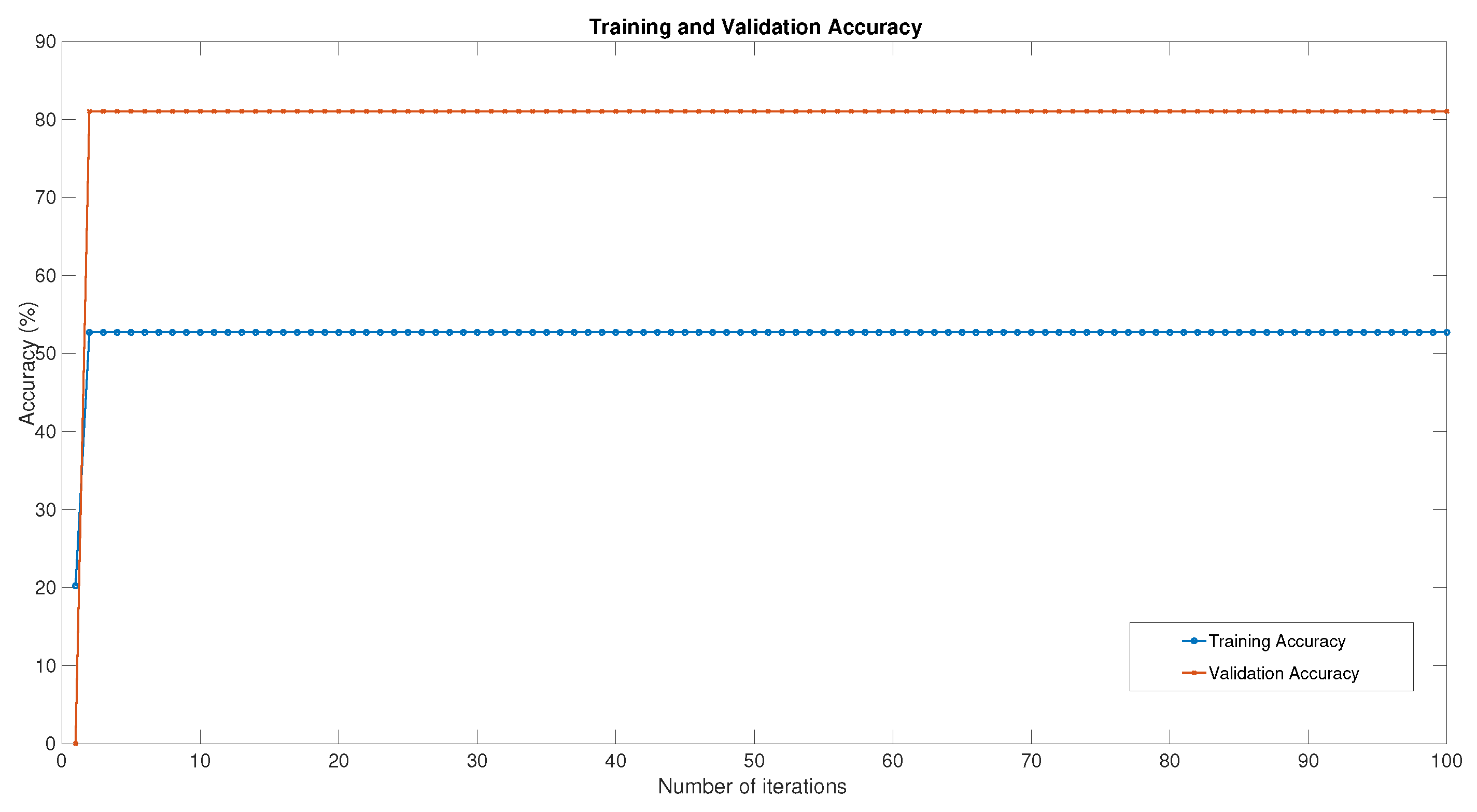
Algorithm (4)	23	0.0787	81.06	100	89.54	81.06

demonstrates that our algorithm is among those with the highest precision, recall, F1-score, and accuracy efficiency. Additionally, it has the lowest number of iterations. Although it may slightly reduce training time, compared to previous examinations, it has the best probability of correctly categorizing prospective mathematics teachers’ technology-integrated competency level. Moreover, we deliver the training and validation loss with the accuracy of training to show that our algorithm has no overfitting in the training dataset.

From Figure 1 and Figure 2, we see that our model from Algorithm 3 with the suitable parameters in Table 2, Table 3 and Table 4 obtains a good fitting model that is the measure of a machine learning model and generalizes well to similar data. Based on Figure 1 and Figure 2, the over fitting problem can be controlled by finding the best parameters of our algorithms to solve the least square regularization problem (28).

We implemented an inertial subgradient extragradient method for the equilibrium problem on an educational dataset of 954 instances containing ten attributes, including major, gender, GPA, IT for learning competency, innovative skill, technology knowledge for a specific subject, number of supplementation, curriculum pattern, selective technology courses and competency level. The accuracy of classification achieved by the proposed machine learning algorithm was evaluated and 81.06% of the dataset was classified accurately with fewer iterations compared to other methods.

5. Conclusions and Discussion

This study proposes a new method based on machine learning algorithms to predict the technology-integrated competency level of prospective mathematics teachers, taking their data related to different aspects as the source data. Performances of an extragradient method for equilibrium problem were calculated and compared to predict the technology-integrated competency. This study emphasized two focuses. The first one was the prediction of competency based on the skills and knowledge developed throughout teacher education programs. The second focus was the comparison of the performances of machine learning algorithm.

The results show that the proposed method achieved a classification accuracy of 81.06%. Accordingly, it can be said that major, gender, GPA, IT for learning competency, innovative skill, technology knowledge for a specific subject, number of supplementation, curriculum pattern, and selective technology courses are significant predictors to be used for predicting their technology-integrated competency.

Even though this study focused on technology-integrated competency in mathematics classrooms, it was noticed that the major of prospective teachers was one of the predictors. Because there is a large number of prospective teachers in Thailand who may teach out of their field upon entering the profession [29], the major of teacher education programs was also analyzed to determine if their technology-integrated competency differs when they are required to teach mathematics in the future [30].

Comparing the results of this study to other studies on technology integration by mathematics teachers, it was discovered that gender is one of the best predictors of teachers’ intentions to implement technology in their classes [31,32]. In addition, general technological skills and knowledge, such as IT for learning competency and innovative skill, are without a doubt effective predictors of technology-integrated competency [25,33,34]. Additionally, the integration of technology knowledge and content knowledge, also known as Technological Content Knowledge (TCK), was represented by the attribute of technology knowledge for a specific subject, which is a predictor for predicting technology-integrated competency [25,34,35].

The curriculum pattern, according to the educational dataset analyzed in this study, is the new finding that distinguishes this study from others. Since Pattern 1, Pattern 2, and Pattern 3 are included in this study—the attributes of the curriculum pattern—there are three sorts of pattern. The patterns that prospective teachers study the most in courses of pedagogical knowledge, content knowledge, and technological knowledge are Pattern 1, Pattern 2, and Pattern 3, respectively. This finding indicates that when prospective teachers were trained in a variety of knowledge patterns, their technology-integrated competency also performed differently [36,37].

Using this approach, it is possible to anticipate future technology-integrated competency based on these findings. By projecting prospective teachers’ technology-integrated competency in the future, pre-service teachers can examine and improve their working techniques and proficiency. Given that there are about four years between teacher education programs, it is easier to comprehend the significance of the proposed strategy.

The practical achievement of this study is a curriculum revision policy for university-level mathematics education programs. Particularly, the program should offer additional TCK courses, and the redesigned curriculum should place a greater emphasis on technology knowledge for mathematics. In addition, the result specifies the concept of the required curriculum pattern in terms of weighing pedagogical knowledge, content knowledge, and technology knowledge courses.

In the comparison of performances of a machine learning algorithm with other methods, it was found that our Algorithm 3 uses fewer iterations than the existing algorithms with the same highest precision, recall, F1-score, and accuracy efficiency and has the same number of iterations compared with Algorithm 3, although it takes slightly less time to train the data. This means that we can choose to use both algorithms to work with these data.

The results demonstrate that machine learning techniques can be used to predict the technology-integrated competency of prospective mathematics teachers. The results of this study can assist educators in identifying pre-service teachers with below or above average technology integration. In addition, such data driven studies are very significant for establishing a prospective teacher competency analysis framework in teacher education and contributing to decision-making for policy design.

Future research can be undertaken by incorporating additional input attributes and machine learning methods into the modeling procedure. In addition, it is crucial to leverage the efficacy of an extra gradient method in order to analyze the learning patterns of individuals, address their issues, enhance the educational environment, and enable data driven decision-making for the policy design of teacher education in Thailand.

References

1. National Council of Teachers of Mathematics. Principles to Actions: Ensuring Mathematical Success for All; National Council of Teachers of Mathematics: Reston, VA, USA, 2014. [Google Scholar]
2. Graham, C.R.; Burgoyne, N.; Cantrell, P.P.; Smith, L.M.; Clair, L.S.; Harris, R. TPACK development in science teaching: Measuring the TPACK confidence of inservice science teachers. TechTrends 2009, 53, 70–79. [Google Scholar]
3. Roshelle, J.; Leinwand, S. Improving student achievement by systematically integrating effective technology. NCSM J. Math. Educ. Leadersh. 2011, 13, 3–9. [Google Scholar]
4. Niess, M.L.; Roschelle, J. Transforming Teachers’ Knowledge for Teaching Mathematics with Technologies through Online Knowledge-Building Communities. In Proceedings of the 40th Annual Meeting of the North American Chapter of the International Group for the Psychology of Mathematics Education, Greenville, SC, USA, 15–18 November 2018; pp. 44–62. [Google Scholar]
5. Ahshan, R. A framework of implementing strategies for active student engagement in remote/online teaching and learning during the COVID-19 pandemic. Educ. Sci. 2021, 11, 483. [Google Scholar] [CrossRef]
6. Hill, H.C.; Rowan, B.; Ball, D.L. Effects of teachers’ mathematical knowledge for teaching on student achievement. Am. Educ. Res. J. 2005, 42, 371–406. [Google Scholar] [CrossRef] [Green Version]
7. Barlovits, S.; Jablonski, S.; Lázaro, C.; Ludwig, M.; Recio, T. Teaching from A Distance—Math Lessons during COVID-19 in Germany and Spain. Educ. Sci. 2021, 11, 406. [Google Scholar] [CrossRef]
8. National Council of Teachers of Mathematics. Catalyzing Change in Middle School Mathematics: Initiating Critical Conversations; National Council of Teachers of Mathematics: Reston, VA, USA, 2020. [Google Scholar]
9. Adipat, S. Developing Technological Pedagogical Content Knowledge (TPACK) through Technology-enhanced Content and Language-Integrated Learning (T-CLIL) instruction. Educ. Inf. Technol. 2021, 26, 6461–6477. [Google Scholar] [CrossRef]
10. Thomas, M.O.J.; Hong, Y.Y. Teacher integration of technology into mathematics learning. Int. J. Technol. Math. Educ. 2013, 20, 69–84. [Google Scholar]
11. Muu, L.D.; Oettli, W. Convergence of an adaptive penalty scheme for finding constrained equilibria. Nonlinear Anal. Theory Methods Appl. 1992, 18, 1159–1166. [Google Scholar] [CrossRef]
12. Blum, E.; Oettli, W. From optimization and variational inequalities to equilibrium problems. Math. Stud. 1994, 63, 123–145. [Google Scholar]
13. Tan, B.; Cho, S.Y. Strong convergence of inertial forward-backward methods for solving monotone inclusions. Appl. Anal. 2021, 101, 1–29. [Google Scholar] [CrossRef]
14. Rehman, H.U.; Kumam, W.; Sombut, K. Inertial modification using self-adaptive subgradient extragradient techniques for equilibrium programming applied to variational inequalities and fixed-point problems. Mathematics 2022, 10, 1751. [Google Scholar] [CrossRef]
15. Muangchoo, K. Three novel two-step proximal-like methods for solving equilibrium and fixed point problems in real Hilbert spaces. Comp. Appl. Math. 2022, 41, 374. [Google Scholar] [CrossRef]
16. Tran, D.Q.; Dung, M.L.; Nguyen, V.H. Extragradient algorithms extended to equilibrium problems. Optimization 2008, 57, 749–776. [Google Scholar] [CrossRef]
17. Korpelevich, G. The extragradient method for finding saddle points and other problems. Matecon 1976, 12, 747–756. [Google Scholar]
18. Censor, Y.; Gibali, A.; Reich, S. Algorithms for the split variational inequality problem. Numer. Algorithms 2012, 59, 301–323. [Google Scholar] [CrossRef]
19. Rehman, H.U.; Kumam, P.; Cho, Y.J.; Yordsorn, P. Weak convergence of explicit extragradient algorithms for solving equilibirum problems. J. Inequalities Appl. 2019, 2019, 1–25. [Google Scholar] [CrossRef]
20. Rehman, H.U.; Kumam, P.; Kumam, W.; Shutaywi, M.; Jirakitpuwapat, W. The inertial sub-gradient extra-gradient method for a class of pseudo-monotone equilibrium problems. Symmetry 2020, 12, 463. [Google Scholar] [CrossRef] [Green Version]
21. Polyak, B.T. Some methods of speeding up the convergence of iteration methods. USSR Comput. Math. Math. Phys. 1964, 4, 1–17. [Google Scholar] [CrossRef]
22. Tiel, J.V. Convex Analysis: An Introductory Text, 1st ed.; Wiley: New York, NY, USA, 1984. [Google Scholar]
23. Auslender, A.; Teboulle, M.; Ben-Tiba, S. A logarithmic-quadratic proximal method for variational inequalities. Comput. Optim. Appl. 1999, 12, 31–40. [Google Scholar] [CrossRef]
24. Bauschke, H.H.; Combettes, P.L. Convex Analysis and Monotone Operator Theory in Hilbert Spaces, 2nd ed.; CMS Books in Mathematics; Springer: Cham, Switzerland, 2017. [Google Scholar]
25. Niess, M.L.; Ronau, R.N.; Shafer, K.G.; Driskell, S.O.; Harper, S.R.; Johnston, C.; Browning, C.; Aslizgn-Koca, S.; Kersaint, G. Mathematics teacher TPACK standards and development model. Contemp. Issues Technol. Teach. Educ. 2009, 9, 4–24. [Google Scholar]
26. Huang, G.-B.; Zhu, Q.-Y.; Siew, C.-K. Extreme learning machine: Theory and applications. Neurocomputing 2006, 70, 489–501. [Google Scholar] [CrossRef]
27. Tibshirani, R. Regression shrinkage and selection via the Lasso. J. R. Stat. Soc. Ser. B Stat. Methodol. 1996, 58, 267–288. [Google Scholar] [CrossRef]
28. Han, J.; Kamber, M.; Pei, J. Data Mining: Concepts and Techniques, 3rd ed.; Morgan Kaufman Publishers: Waltham, MA, USA, 2012; p. 978. [Google Scholar]
29. Ingersoll, R. A comparative study of teacher preparation and qualifications in six nations. CPRE Policy Briefs 2007, 47, 1–16. [Google Scholar]
30. Ndlovu, M.; Ramdhany, V.; Spangenberg, E.D.; Govender, R. Preservice teachers’ beliefs and intentions about integrating mathematics teaching and learning ICTs in their classrooms. ZDM 2020, 52, 1365–1380. [Google Scholar] [CrossRef]
31. Anderson, S.E.; Maninger, R.M. Preservice teachers abilities, beliefs, and intentions regarding technology integration. J. Educ. Comput. Res. 2007, 37, 151–172. [Google Scholar] [CrossRef]
32. Raman, A.; Thannimalai, R. Importance of technology leadership for technology integration: Gender and professional development perspective. SAGE Open 2019, 9, 1–13. [Google Scholar] [CrossRef] [Green Version]
33. Niess, M.L. Investigating TPACK: Knowledge growth in teaching with technology. J. Educ. Comput. Res. 2011, 44, 299–317. [Google Scholar] [CrossRef]
34. Bonafini, F.C.; Lee, Y. Investigating prospective teachers TPACK and their use of mathematical action technologies as they create screencast video lessons on iPads. Techtrends 2021, 65, 303–319. [Google Scholar] [CrossRef]
35. Mouza, C.; Karchmer-Klein, R.; Nandakumar, R.; Ozden, S.Y.; Hu, L. Investigating the impact of an integrated approach to the development of preservice teachers’ Technological Pedagogical Content Knowledge (TPACK). Comput. Educ. 2014, 71, 206–221. [Google Scholar] [CrossRef]
36. Durak, H.Y. Preparing pre-Service teachers to integrate teaching technologies into their classrooms: Examining the effects of teaching environments based on open-ended, hands-on and authentic tasks. Educ. Inf. Technol. 2021, 26, 5365–5387. [Google Scholar] [CrossRef]
37. Ratnayake, I.; Thomas, M.; Kensington-Miller, B. Professional development for digital technology task design by secondary mathematics teachers. ZDM 2020, 52, 1423–1437. [Google Scholar] [CrossRef]
Figure 1. Accuracy plots of the iteration of Algorithm 3 from Table 5.
Mathematics 10 04464 g001
Figure 2. Loss plots of the iteration of Algorithm 3 from Table 5.
Mathematics 10 04464 g002