Three-Branch Random Forest Intrusion Detection Model

Abstract

Network intrusion detection has the problems of large amounts of data, numerous attributes, and different levels of importance for each attribute in detection. However, in random forests, the detection results have large deviations due to the random selection of attributes. Therefore, aiming at the current problems, considering increasing the probability of essential features being selected, a network intrusion detection model based on three-way selected random forest (IDTSRF) is proposed, which integrates three decision branches and random forest. Firstly, according to the characteristics of attributes, it is proposed to evaluate the importance of attributes by combining decision boundary entropy, and using three decision rules to divide attributes; secondly, to keep the randomness of attributes, three attribute random selection rules based on attribute randomness are established, and a certain number of attributes are randomly selected from three candidate fields according to conditions; finally, the training sample set is formed by using autonomous sampling method to select samples and combining three randomly selected attribute sets randomly, and multiple decision trees are trained to form a random forest. The experimental results show that the model has high precision and recall.

1. Introduction

Rapid progress has been made in science and technology, and networking has been accelerating. While the network provides convenience for people’s lives, the security problem is increasingly prominent. Once a security incident occurs, it causes significant economic losses and social impact. To increase the stability of the network defense system, new intrusion detection models need to be constantly studied and improved to improve the overall performance of the intrusion detection system. With the rapid development of machine learning, many scholars began to study the application of machine learning to intrusion detection, such as decision trees [1,2], support vector machines [3], Bayesian networks [4,5], K-nearest neighbors [6], etc. and constantly put forward improvement measures for algorithms. As a common algorithm used in intrusion detection, decision tree has achieved good results in intrusion detection. With the improvement and development of different detection models in recent years, traditional machine learning has exposed many drawbacks. A single machine learning algorithm is often prone to have some blind spots, resulting in low detection accuracy, poor discrimination, and other problems. Therefore, ensemble learning gradually appeared in the field of intrusion detection. Ensemble learning trains multiple classifiers, and then integrates individual classifiers through certain strategies to obtain a stable model that performs well in all aspects. The intrusion detection methods of ensemble learning are mainly divided into AdaBoost [7] and bagging [8]. The intrusion detection algorithm based on AdaBoost generates bad base classifiers with the increase of learners, which leads to the decline of integration performance and affect the performance of intrusion detection. Bagging-based intrusion detection mainly includes intrusion detection based on random forest. As a typical ensemble learning model, random forest is an algorithm obtained by integrating multiple decision trees. At present, many scholars have applied it to intrusion detection. For example, in [9], considering that the traditional ensemble learning algorithm cannot accept all training samples at one time due to the continuous generation of new attacks in intrusion detection, the idea of semi-supervision is introduced into ensemble learning. The bootstrap method is used for placing back sampling to obtain base classifiers and selectively labeled samples, which improves the detection accuracy of the model. The literature [10] defines the concept of approximate reduction, divides the attributes of the dataset, and trains them separately to obtain a base classifier with significant differences, which ensures the generalization of the final integrated learner. To solve the overfitting phenomenon, study [11] proposed an improved network intrusion detection method of random forest classifier by increasing the diversity of random forests through the Gaussian mixture clustering algorithm. Reference [12] proposed an intrusion detection algorithm based on random forest and artificial immunity to solve the problems of low detection rate of traditional intrusion detection methods for network intrusion attack types such as Probe, U2R, R2L, and false detection and missing detection of intrusion behaviors. Reference [13] proposed a network intrusion detection model based on random forest, and achieved good results in detection rate. Reference [14] proposed the combination of extreme gradient lifting tree and random forest, built an intrusion detection model, improved the random forest algorithm, and dealt with the problem of data imbalance, and finally the detection accuracy was effectively improved.

Intrusion detection datasets usually have many attributes, and not every attribute is equally essential. In a random forest, the probability of selecting attributes with high importance and attributes with low importance is the same. If the likelihood of attributes with high importance being chosen increases, the classification effect of the decision tree will increase accordingly. Therefore, considering the impact of different attribute importance on the final classification accuracy, it is necessary to increase the probability of selecting essential attributes in the intrusion detection dataset. The measurement method of attribute importance is not unique, such as attribute importance based on information entropy [15], attribute importance based on rough set [16,17,18,19,20], etc. When most methods improve the importance of attributes, they directly delete the attributes with low importance, which leads to the loss of data information to a certain extent.

Three decision [21,22,23] refers to the addition of a delayed decision based on the original two decisions. This decision method is to delay judgment of the original uncertain decision. This paper is just to integrate this idea into attribute selection, rejudge some attributes, and propose an attribute selection method based on three-branches of decision-making and attribute importance, fully consider the complexity and uncertainty of data, divide the data into the positive domains, negative domain, and boundary domain, and randomly select a certain number of attributes from the three domains, which not only gives priority to attribute importance, but also ensures the randomness of attributes through attribute selection. According to different attribute subsets obtained from three decisions, the decision tree is trained. The multiple decision trees obtained from the training are integrated according to the voting method, and the three-branch random forest integration model is obtained.

To sum up, the attribute measurement method based on decision boundary entropy is used to calculate the importance, taking into account the information of positive domain and boundary domain at the same time, and then three randomized decision methods of attributes are used to select attributes to ensure the randomness of attribute selection. Finally, the attribute subsets obtained are divided into decision trees, and finally IDTSRF models are integrated and used for intrusion detection. The recall rate and F1 value are selected as the main evaluation indicators in the experiment. Compared with random forest, AdaBoost, XGBoost, extra trees, CNN and CNN-LSTM, the results show that IDTSRF achieves high recall and F1 value.

2. Related Work and Background Work

2.1. Intrusion Detection Based on Machine Learning

The main work of intrusion detection system is to detect and process the possible behaviors in the network. With the rapid development of machine learning, many researchers are trying to apply machine learning algorithms to intrusion detection. By analyzing and learning the existing detection data, they can find its internal structure and rules to detect abnormal behaviors in the network. This method can not only detect the existing attack types in the training set but also detect new attacks that have not occurred by learning data characteristics, which has predictive ability to a certain extent. The intrusion detection system based on machine learning includes supervised learning and unsupervised learning. Supervised learning includes support vector machines (SVM) [3], naive Bayesian classifiers [24], and decision trees [2], while unsupervised learning includes k-means clustering [25], association rules [26], self-organizing map neural networks (SOM) [27]. Through continuous research, development and improvement, some algorithms of deep learning are also gradually applied to intrusion detection, such as deep belief networks (DBN) [28], convolutional neural networks (CNN) [29], recurrent neural networks (RNN) [30] and other algorithms, but the above methods are all based on a single classifier for experiments, and this single classifier often cannot achieve the desired classification effect, and classification performance and robustness are relatively weak. As a kind of machine learning, ensemble learning is just assembling multiple single classifiers into a stable model that performs well in all aspects according to certain rules. This model can alleviate the problems of the previous single-classifier detection model to a certain extent. Therefore, some scholars began to consider applying ensemble learning to intrusion detection in 2003. Since then, many intrusion detection algorithms about ensemble learning have been proposed [31]. It mainly includes adaptive boosting [32], extreme gradient boosting (XGBoost) [33], random forests (RF) [34], etc. Figure 1 summarizes some machine learning algorithms currently used in intrusion detection.

• SVM

SVM is mainly used to solve regression and classification problems. The algorithm takes the data points in the space as input and finally obtains a hyperplane to classify the samples. The partition condition is to maximize the interval to obtain better generalization ability.

2.

Naive Bayes

Naive Bayes is a probability algorithm which believes that each attribute is independent. By estimating the probability of the occurrence of each category and attribute, the maximum-likelihood estimation is used to calculate the maximum probability as the final result.

3.

Decision tree

A decision tree selects sample features through information gain method. It stores the sample features in the tree structure for hierarchical sorting and finally generates the decision tree based on the attribute test conditions represented by its nodes. In order to prevent overfitting, the decision tree is also pruned.

4.

K-means clustering

K-means clustering needs to first select k sample points as the center point, then calculate the distance between all samples and the center point to divide into clusters and then recalculate the center point according to the sample points in the cluster and repeat this operation until the center point and distance value no longer change.

5.

Association Rules

Association rules can find associations or connections in data for division. First, you need to filter the data, then find frequent item sets according to confidence, and finally find strong association rules from them.

6.

Self-Organizing Map Neural Network

An SOM is a two-layer neural network which is trained by competitive learning. By finding the active node of each input sample, updating the node parameters and adjusting the connection weight of neurons, the clustering result is finally obtained.

7.

Deep Belief Network

DBN is a hybrid generation model composed of restricted Boltzmann machine and Sigmaid belief network. It can identify, classify, and generate data by training the weight between its neurons.

8.

Convolutional Neural Network

A CNN performs dimension reduction and feature extraction through convolution layer, and sampling operation is performed by pooling layer, which plays the role of reducing computation and improving generalization capability. Finally, classification occurs through the full connected layer.

9.

Recurrent Neural Network

An RNN can effectively process data with sequence characteristics. A CNN extracts features by means of convolution and RNN extracts features by means of cyclic kernel and then sends them to subsequent networks for prediction and other operations.

10.

AdaBoost

AdaBoost can train the same training set to get different classifiers by adjusting the weights. Finally, the weak classifiers are assembled into strong classifiers by some methods.

11.

XGBoost

XGBoost is an additive model. The forward distribution algorithm is used to gradually optimize the internal base learners. Each base learner is a regression tree. Finally, the objective function is written to solve the optimal value.

2.2. Related Work with Machine Learning

This paper mainly divides machine learning into three aspects: supervised learning, unsupervised learning, and ensemble learning. In supervised learning, the algorithm needs to learn the mapping rules from input to output on labeled data samples containing normal samples and abnormal samples. The disadvantage is that the supervised learning algorithm has low detection rate for unknown attacks. Moreover, the label accuracy of labeled samples cannot be guaranteed, and the data contain noise, which may lead to a high false alarm rate of the model. Compared with supervised learning, unsupervised learning can better detect location attacks and does not use tag data. It can classify data according to two hypothetical functions without any prior knowledge [35]. The emergence of ensemble learning has solved the problem that a single classifier only performs well in some aspects. It combines multiple weak supervision models and their advantages in a certain way to form a strong supervision model. Machine learning is applied to intrusion detection, and network data is classified into normal data and abnormal data. The machine learning intrusion detection model is divided into data preprocessing, feature learning, model selection, and training. The final classifier is used for intrusion detection verification with test set. A test process is shown in Figure 2.

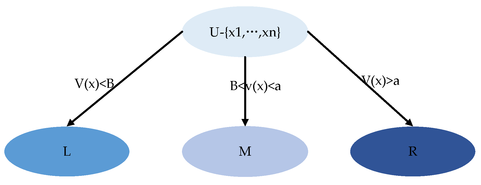
2.3. Three-Branch Decision Making Based on an Evaluation Function

• Three decisions:

Compared with the two branches, the three-branches of decision-making are more in line with human decision-making methods, and it adds delayed decision-making based on the two branches of decision-making. The classification labels of the two classifications are $POS$ (Accept) or $NEG$ (Reject), and the three decisions add $BND$ (Delay Decision), whose decision sets are represented as $D=\left\{D_P,D_B,D_N\right\}$, $D_P,D_B,D_N$ represent acceptance, boundary, and rejection decisions respectively. By calculating the losses under the three actions of $D_P,D_B$ and $D_N$, calculate the thresholds $\alpha$ and $\beta$. Finally, judge the classification label of the current sample. The judgment rules are as follows:

• If $P\left(X|\left[x\right]\right)\ge \alpha$, $x\in POS\left(X\right)$;
• If $\beta <P\left(X|\left[x\right]\right)<\alpha$, $x\in BND\left(X\right)$;
• If $P\left(X|\left[x\right]\right)\le \beta$, $x\in NEG\left(X\right)$ [36].

• Three-branch decision making based on evaluation function:

To make three decisions, entities need to be divided according to thresholds and decision functions. By mapping $f$, the entity set $U$ is divided into three domains: $L$, $M$ and $R$. These three domains are disjoint, and corresponding rules are constructed based on these three domains. The decision function is also called the evaluation function. The evaluation function is divided into a single evaluation function $f=v\left(x\right)$ and multiple evaluation functions $f=\left\{v_1\left(x\right),\dots \dots ,v_k\left(x\right)\right\}$. The evaluation functions in different domains can be the same or different. The range of evaluation function is divided into a totally ordered set, partially ordered set, and lattice. The single evaluation function based on total order is divided into three domains by the threshold $\left(\alpha ,\beta \right)$. Assuming $\alpha \ge \beta$, the division rules are as follows:

• If $v\left(x\right)<\beta$, it belongs to $L-$ domain;
• If $\alpha \le v\left(x\right)\le \beta$, it belongs to the $M-$ domain;
• If $v\left(x\right)>\alpha$, it belongs to $B-$ domain.

The state diagram is shown in Figure 3.

Wu Qirui [37] and others proposed a method to combine convolutional neural network with three-branches of decision-making. They entirely used the superior feature extraction ability of convolutional neural network and the ability of three-branches of decision-making to avoid blind classification, and delayed decision making on data that could not be made in time, that is, feature extraction again. The experiment shows that this method improves the performance of intrusion detection system as a whole. Du Xiangtong [38] and others used deep belief networks to extract features many times to build a multi-granularity feature space, then used three decision theories to make timely decisions on intrusion or normal behaviors, and used KNN classifiers to further analyze uncertain network behaviors within the boundary domain of the three decision theories to obtain detection results. This model further improved the performance of the intrusion detection system. Zhang Shipeng [39] and others used a noise reduction self-encoder to extract features from high-dimensional data, and then made immediate decisions using three decision theories to further analyze and judge boundary domain data, effectively avoiding the risk of blind classification. To sum up, most current intrusion detection models based on three decisions only consider further re-judgment of uncertain network data by using the delay decision in the three-way decision theory, ignoring the problem that different attribute importance of network data leads to different impacts on classification results. Therefore, this paper proposes three decision intrusion detection methods considering the importance of attributes and improves the measurement method of attribute importance of data with decision boundary entropy to improve the performance of intrusion detection systems further.

2.4. Random Forest

Stochastic forest is an essential method in ensemble learning which can be used for classification, regression, dimension reduction, abnormal data processing, etc. It is formed by many unrelated decision tree sets. Each tree depends on the vector value of random sampling. It needs to randomly sample the experimental sample set to generate a large number of sample subsets, and randomly select the attribute characteristics of the sample set. These two processes have great randomness. Finally, we need to train many decision trees according to these subsets, and then vote for the final result according to the results. After being proposed, random forest has quickly become a research hotspot in data mining [40], pattern recognition [41], artificial intelligence [42], and other fields because of its advantages of no overfitting, high prediction accuracy, and strong noise resistance.

The generation rules of each tree in the random forest are as follows:

• Set the training set size as $M$. For each tree, $M$ training samples are randomly and put back from the training as the training set of the tree. Repeat $N$ times to generate the training sample set of $N$ group.
• If the sample dimension of each feature is $k$, specify a constant $l$<<$k$, (usually $l=\sqrt{k}$) and randomly select $l$ features from the $k$ features.
• Use $l$ features to maximize the growth of each tree, and there is no pruning process.
• The final integration is obtained by integrating the prediction results of all trees.

The most distinctive features of random forest are data randomness and attribute randomness. The role of data randomness is to conduct self-service and back sampling on the original data, and back sampling can ensure that the datasets obtained have both differences and will not be too different, ensuring the diversity of trees. The role of attribute randomness is to select $\sqrt{k}$ attributes randomly from all attributes as candidate attributes and select the best attribute as the partition node to train the optimal learning model, which further enhances the diversity of the tree [43]. These two randomnesses ensure that the model has a certain anti-noise ability, and it is not easy to fall into overfitting. However, the selection of the two randomnesses causes some shortcomings. For example, if all attributes are selected randomly, the difference in attribute importance is ignored, which directly affects the accuracy of the final classifier. This experiment is based on this point, considering the selection of attributes based on importance, and for the attributes that cannot be determined immediately, the delayed decision is added for re-judgment, which effectively improves the problem caused by the randomness of attributes. The traditional random forest model is shown in Figure 4.

2.5. Related Work with Non-ML Techniques

In addition to the machine learning algorithms mentioned above, the application of some non-machine learning algorithms in intrusion detection has been constantly explored and improved in recent years.

• Reference [44] proposed a method combining multiple criteria linear programming (MCLP) and particle swarm optimization (POS). The main idea of MCLP is to seek to minimize and separate the sum of all overlaps of hyperplanes and maximize the sum of distances from points to the separation hyperplane [45]. However, the algorithm easily affects performance due to improper parameter selection and adjustment in the implementation process, so it is proposed to apply particle swarm optimization to parameter adjustment. Its advantages are less computation and the ability to find the global optimum. POS algorithm updates the velocity and position of each particle iteratively according to its own experience (pbest) and the best experience of all particles (gbest) and finally stops the iteration to obtain the best MCLP parameters. The experimental results also show that compared with a single MCLP model, the method in this paper effectively improves the detection accuracy and reduces the detection time. However, this method requires high data and does not consider the impact of too high dataset dimensions.
• Reference [46] proposed an intrusion detection model based on ant colony optimization (ACO) for feature selection. In this paper, features are regarded as nodes in the ACO algorithm, and the connection between nodes represents the next feature selection. Then, the graph is searched for the optimal feature subset through ant colony traversal. Finally, the optimal feature subset is obtained by applying the transformation rules and pheromone update rules of the ACO algorithm. Experimental results show that the algorithm achieves higher detection rates. However, when the data and distribution are uneven, the results of this method may be affected.

2.6. Correlation Comparison Algorithm

For the three-branch random forest model, several different ensemble learning algorithms and deep learning algorithms are selected for experimental comparison. The advantages and disadvantages of all methods are shown in

Table 1. Advantages and disadvantages of the model.

Model		Introduce
IDTSRF	The advantage is that different attributes in the dataset have different effects on the results. Therefore, attribute importance measurement method based on decision boundary is adopted to select attributes and finally the attribute subset training decision tree integrated random forest model is obtained.	The disadvantage is that this method has better detection effect on small datasets at present. The next step will be to study this.
Random Forest	The advantage is that the idea of ensemble learning is adopted, which improves the accuracy of a single algorithm, is more stable, and does not easily fall into over fitting.	The disadvantage is that the calculation cost is high, requiring more time and space.
XGBoost	The advantage is that the regular term is introduced to reduce the complexity of the model, support parallel processing and high flexibility, and reverse pruning from bottom to top makes the model not easily fall into the optimal solution.	The disadvantage is that more model parameters lead to complex parameter adjustment, which is difficult to deal with with ultra-high dimensional data.
AdaBoost	The advantage is that different classifiers can be used as weak classifiers, and weak classifiers can be cascaded to fully consider the weight of each classifier.	The disadvantage is that the data imbalance easily affects the classification accuracy of the model and consumes time.
CNN	The advantage is that the shared convolution kernel can better handle high-dimensional data and can automatically extract features.	The disadvantage is that with the deepening of the network layer, the time is also extended, and the pooling layer loses a lot of useful information when compressing features.
SVM	The advantage is that the learning effects is good on small samples, and it can solve high-dimensional problems well, with good generalization.	The disadvantage is that it supports two classifications. When the sample size is too high, the calculation increases, which consumes a lot of memory and time.
Naive Bayesian	The advantages are excellent performance on small datasets, and it can handle multi-classification tasks and simple algorithms for implementation.	The disadvantage is that prior probabilities and assumptions need to be known while attributes are relatively independent, which affects the classification effect.
Decision Tree	The advantage is that the nominal and numerical data can be processed at the same time and the model training is fast and efficient.	The disadvantage is that it is easy to overfit, and the classification results are easily affected by the distribution of the number of samples, so the decision tree needs to be trained after data processing.
K-means	The advantages are fast convergence speed and simple parameters.	The disadvantage is that it easily falls into the local optimum, the K value and the center point are not easy to determine, and the data types are limited to seek the mean value.
Association Rules	The advantage is that it is not limited by the amount of data and can find the relationship between data in a large amount of data with a wide range of applications.	The disadvantage is that the analysis takes a long time, takes a large amount of memory, and does not take into account the different importance of attributes.
SOM	The advantage is that the visualization effect is good and is not easily affected by the initial parameter selection.	The disadvantage is that there is no definite objective function and the computational complexity is high.
DBN	The advantage is good flexibility.	The disadvantage is that it can only deal with one-dimensional data and easily falls into local optimum.
RNN	The advantage is that previous information is considered, which is suitable for processing sequential data.	The disadvantages are high video memory occupation, difficult training, gradient disappearance, and gradient explosion.

.

2.7. Problem Description

• The traditional machine learning algorithm has blind spots and has a certain tendency. Try to apply the integrated learning idea, and a single model is integrated to generate a stable model with excellent performance in all aspects;
• The attributes of the intrusion detection dataset are not unique, and different attributes have different effects on the classification results. Therefore, a method is adopted to calculate the importance of different attributes to increase the probability that the attributes with higher importance are selected;
• Most of the traditional attribute importance measurement methods directly delete the attributes with low importance, which to some extent leads to the loss of information. Therefore, a method needs to be adopted to judge and select the attributes with different importance.

3. Three-Branch Random Forest Intrusion Detection Model

3.1. IDTSRF Intrusion Detection Model Framework

Figure 5 is the overall framework of the intrusion detection algorithm based on three-way selected random forest (IDTSRF).

As shown in Figure 5, the steps of the IDTSRF intrusion detection model are as follows:

4.

A hierarchical sampling of the original dataset in proportion;

5.

Because the dataset contains continuous attributes, according to the characteristics of different attributes, the data are discretized using equal distance dispersion or equal frequency dispersion to obtain the dataset $D$ required by the experiment;

6.

Self-service sampling is performed on the dataset $D$ to generate $N$ data subsets $D_1,D_2,\cdots ,D_N$ and off-package data;

7.

Set the evaluation function of the attribute based on the attribute importance of decision boundary entropy ($DBE$), give the value of threshold value to $(\alpha ,\beta )$, and divide the attributes in all data subsets into a positive domain, boundary domain or negative domain, respectively;

8.

Select $\sqrt{k}$ attributes according to three attribute selection rules (see Section 3.3);

9.

The GINI index is selected as the criteria for node division of the decision tree to generate a $N$ tree;

10.

The majority voting method is adopted to integrate the results to get the final integration;

11.

To verify the effectiveness of the algorithm, test data are input into the integration to verify the effectiveness of the algorithm.

The critical problem of the IDTSRF intrusion detection model is to calculate the importance of attributes and the three choices of attributes and design an improved random forest algorithm based on this.

3.2. Decision Boundary Entropy and Attribute Importance

In the IDTSRF intrusion detection model, attribute importance is redefined based on decision boundary entropy, which is used as an evaluation function to construct three attribute decisions, and attributes are divided into positive domain, negative domain, and boundary domain candidate domains.

Definition 1.

(Decision Boundary Entropy, DBE) [43] Given a decision table $DT=(U,C,D,V,f)$, $U/IND(D)=\{D_1,D_2,\cdots ,D_m\}$, $\forall B\subseteq C$, the decision boundary entropy of $D$ related to $B$ is defined as [43]:

$$DBE(D,B)=(1-{\alpha }_B(D))\times {\displaystyle \sum _{i=1}^m\frac{\left|BN{D}_B(D_i)\right|}{\left|U\right|}{\log }_2}\left(\frac{\left|BN{D}_B(D_i)\right|}{\left|U\right|}+1\right)$$

(1)

where, ${\alpha }_B(D)$ represents approximate classification accuracy and $BN{D}_B(D_i)$ represents boundary region.

Definition 1 uses approximate classification precision and $\frac{\left|BN{D}_B(D_i)\right|}{\left|U\right|}$ to construct decision boundary entropy. First, because the boundary domain is the way to estimate uncertainty information in rough sets, Shannon’s information entropy is also the way to measure uncertainty information, so it is feasible to combine $\frac{\left|BN{D}_B(D_i)\right|}{\left|U\right|}$ with entropy to define the decision boundary entropy; secondly, because $\frac{\left|BN{D}_B(D_i)\right|}{\left|U\right|}$ provides information from the boundary domain [43], and the approximate classification quality provides information from the positive domain, combining the two to define the decision boundary entropy, it can effectively integrate the information in the positive domain and the boundary domain and obtain a new standard to measure the quality of attributes.

It can be seen from the definition that the decision boundary entropy is inversely proportional to ${\alpha }_B(D)$ and is proportional to $\frac{\left|BN{D}_B(D_i)\right|}{\left|U\right|}$.

Definition 2.

(attribute importance based on $DBE$) [43] gives a decision table $DT=(U,C,D,V,f)$. For $\forall B\subset C,a\in C-B$, attribute $a$, the attribute importance of $B$ and $D$ is defined as:

$$Sig(a,B,D)=DBE(D,B-\{a\})-DBE(D,B)$$

(2)

In the IDTSRF intrusion detection model, the $DBE$-based attribute importance is used as the evaluation function to construct three attribute decisions. The attributes are divided into three candidate domains: positive domain, negative domain, and boundary domain.

3.3. Randomized Three-Branch Decision of Attributes

Set decision table $DT=(U,C,D,V,f)$, where $U$ represents a nonempty finite set containing all instances, called universe; $C=\{a_1,a_2,\cdots ,a_k\}$ represents $k$ condition attributes; $D=\{d_1,d_2,\cdots ,d_m\}$ represents $m$ decision attributes; $V$ is attribute value, $f:A\to V$ is a mapping [43].

Definition 3.

(Indispensable attribute) Ref. [43] gives a decision table $DT=(U,C,D,V,f)$. For $\forall c\in C$, if $DBE(D,C)\ne DBE(D,C-\{c\})$, it is said that $c$ is an indispensable attribute of $D$ on $C$. Otherwise, $c$ is an unnecessary attribute of $D$ on $C$.

Definition 4.

(Core) [43]. Given a decision table $DT=(U,C,D,V,f)$ and $\forall B\subset C$, for each $b\in B$ and $c\in C-B$, $b$ is an indispensable attribute of $D$ on $C$, and $c$ is an unnecessary attribute of $D$ on $C$. $B$ is called a core of $D$ on $C$.

Definition 5.

(Reduction) Ref. [43] gives a decision table $DT=(U,C,D,V,f)$ and $\forall R\subset C$. If $DBE(D,R)=DBE(D,C)$, for each $b\in R$, there is $DBE(D,R-\{b\})>DBE(D,C)$, and $R$ is called a reduction on $C$ related to $D$ [47].

To make three choices for $DT=(U,C,D,V,f)$ the attribute of the decision table, the evaluation function $F(x)=Sig(a,C,D)$. For $\forall a\in C$, when $Sig(a,C,D)\ge \alpha$, the attribute $a$ is divided into positive decision domain $POS$; when $Sig(a,C,D)\le \beta$, attribute $a$ is divided into negative decision domain $NEG$; when $\beta <Sig(a,C,D)<\alpha$, the attribute $a$ is divided into delay decision domain $BND$. So, there are

$$\{\begin{array}{l}POS=\{a\in C\mid Sig(a,C,D)⩾\alpha \}\hfill \\ BND=\{a\in C\mid \beta <Sig(a,C,D)<\alpha \}\hfill \\ NEG=\{a\in C\mid Sig(a,C,D)\le \beta \}\hfill \end{array}$$

(3)

After the attribute is divided into three domains, to make the attribute selection random, the following three attribute selection rules are defined:

• If $\left|POS\right|>(1+\delta )\sqrt{k}$, randomly select $\sqrt{k}$ attributes from the positive field as attribute subsets;
• If $\left|POS\right|+\left|BND\right|>(1+\delta )\sqrt{k}$, randomly select $\sqrt{k}$ attributes as attribute subset from positive domain and boundary domain [43];
• If $\left|POS\right|+\left|BND\right|\le (1+\delta )\sqrt{k}$, randomly select $\frac{\left|POS\right|+\left|BND\right|}{\sqrt{k}}$ attributes from the positive domain and boundary domain, and randomly select $\left(1-\frac{\left(\left|POS\right|+\left|BND\right|\right)}{k}\right)\sqrt{k}$ attributes from the negative domain to form an attribute subset [43].

Note: The application priority of the three rules is (1) > (2) > (3).

where, $k=\left|POS\right|+\left|BND\right|+\left|NEG\right|$ represents the total number of attributes, $\left|POS\right|,$$\left|BND\right|$, and $\left|NEG\right|$ represent the number of attributes in the positive domain, boundary domain, and negative domain, respectively. In random forests, $\sqrt{k}$ attributes are generally used to train decision trees, and here $\sqrt{k}$ attributes are also used to train decision trees [43].

The theoretical value range of $\delta$ is $(0,\sqrt{k}-1)$. The coefficient $(1+\delta )$ of $\sqrt{k}$ is set to make the number of attributes included in the candidate attribute greater than $\sqrt{k}$. When $\delta =0$, $\sqrt{k}=|POS|$ (or $\left|POS\right|+\left|BND\right|=\sqrt{k}$), there is only one attribute combination provided by candidate attribute set in $POS$ (or $POS\cup BND$), and there is no randomness [43]. With the increase of $\delta$ value, $\left|POS\right|>(1+\delta )\sqrt{k}$ (or $\left|POS\right|+\left|BND\right|>(1+\delta )\sqrt{k}$), the number of candidate attribute set attributes increases, attribute randomness increases, and the fault tolerance and robustness of individual learners increase. On the contrary, the accuracy of individual learners decreases. When $\delta$ is large enough, the number of attributes in the candidate attribute set can only meet rule (3), the randomness of attributes is the best, and the accuracy of individual learners is the worst.

3.4. Three-Branch Attribute Selection random forest Algorithm

In the IDTSRF intrusion detection model, the key is to select and integrate three attributes in random forest algorithm. To this end, a new random forest algorithm is constructed based on three-attribute selection, which is described as follows (Algorithm 1):

Algorithm1: Three-branch attribute selection random forest algorithm

Three-branch attribute selection random forest algorithm Input: Decision tables $DT=(U,C,D,V,f)$, Three attribute selection thresholds $(\alpha ,\beta )$, Attribute randomness $\delta$ Output: TSRF (Forest) 1 For $j=1,2,\cdots ,N$ 2      $U_j=Bootstrap\_Sample\left(U\right)$ 3      Initialization $POS=\{\varnothing \},BND=\{\varnothing \},NEG=\{\varnothing \}$ 4      For $a\in C$ do 5          Calculate $F(a)$ according to formula (2) 6          If $F(a)>\alpha$ then 7              $POS\leftarrow a$ 8          Else 9                If $\beta <F(a)<\alpha$ then 10                  $BND\leftarrow a$ 11             Else 12                  $NEG\leftarrow a$ 13             End if 14          End if 15      End for 16      If $\left|POS\right|>(1+\delta )\sqrt{k}$ 17          Randomly select $\sqrt{k}$ attributes from the positive field to form attribute set $A$ 18      Else 19          If $\left|POS\right|+\left|BND\right|>(1+\delta )\sqrt{k}$ 20              Randomly select $\sqrt{k}$ attributes from positive domain and boundary domain to form attribute set $A$ 21          Else 22              Select $\frac{\left|POS\right|+\left|BND\right|}{k}\sqrt{k}$ attributes from the positive domain and boundary domain, and $\frac{\left|NEG\right|}{k}\sqrt{k}$ attribute structural sets $A$ from the negative domain 23          End if 24        End if 25      $U^{\ast }=$ Dataset with attribute $A$ 26 End for 27 Training decision tree according to $U_1^{\ast },U_2^{\ast },\cdots ,U_N^{\ast }$ 28 Comprehensive results

The algorithm consists of two parts. The first part is to select three attributes to form a dataset. Step 2 is to conduct self-service sampling on the original dataset to generate different datasets of $N$ group. Steps 4 to 15 are to select three attributes, in which Step 5’s Formula (2) calculates the importance of each attribute, and Steps 6 to 15 set the threshold $(\alpha ,\beta )$, construct three decisions, divide the attributes of $k$ into positive domain, boundary domain, and negative domain; the time complexity is $O(2k)$ [43]. Steps 16 to 24 randomly select the attributes, set the attribute randomness threshold $\delta$, and select the attributes in the three fields according to the size of $(1+\delta )\sqrt{k}$ according to the random selection rules to obtain the attribute set $A$. Output the dataset $U_1^{\ast },U_2^{\ast },\cdots ,U_N^{\ast }$ containing the attribute $A$, with the time complexity of $O(1)$. If each dataset includes $n^{\ast }$ samples, the time complexity of Steps 4 to 24 is $O(Nk{n}^{\ast })$;

The second part is to train and integrate decision trees. Step 28 trains $U_1^{\ast },U_2^{\ast },\cdots ,U_N^{\ast }$ into $N$ CART trees. If the depth of CART is $d$, the time complexity of a single CART tree is $O(\sqrt{k}d{n}^{\ast })$, and the time complexity of $N$ CART tree is $O(N\sqrt{k}d{n}^{\ast })$. Step 29 combines the trained trees according to the voting method to get the final classification result.

Based on the above analysis, the time complexity of the algorithm is $O(Nk{n}^{\ast })+O(N\sqrt{k}d{n}^{\ast })$, and because $k\ge d\sqrt{k}$, the time complexity is actually $O(Nk{n}^{\ast })$ [43].

3.5. Data Set and Experimental Environment

KDD CUP 99 is the intrusion detection dataset adopted by KDD competition in 1999. The NSL-KDD dataset used in this article has been partially improved. In view of the shortcomings of KDD CUP 99 dataset, the NSL-KDD dataset removes redundant data from the KDD CUP 99 dataset, overcomes the problem that the classifier tends to repeat records, and the performance of learning methods is affected. In addition, the proportion of normal and abnormal data is properly selected, and the number of test and training data is more reasonable [48], so it is more suitable for effective and accurate evaluation between different machine learning technologies.

The NSL-KDD dataset contains four types of exceptions, a total of 42 features, including 9 basic TCP connection features, 13 TCP connection content features, 9 time-based network traffic statistics features, 10 host-based network traffic statistics features, and 1 label feature. The distribution of datasets is shown in

Table 2. Data type distribution table.

Data Type	Training Set	Test Set
Normal	67,334	9711
DoS	45,927	7458
Probe	11,656	2421
R2L	995	2754
U2L	52	200
Total	125,973	22,544

.

The experiment is based on Intel Xeon W-2123 processor, Windows Server 2019 operating system, and Python 3.7.9 version is used for code design.

3.6. Subsection Data Preprocessing

Most attribute values in the original data are continuous data, and the data are discretized by equal distance dispersion or equal frequency dispersion. Discretization processing is because there is no way to directly use continuous variables in the decision tree, and the NSL-KDD dataset has 41 attribute features. All but 9 discrete features are continuous attributes. Therefore, continuous attributes need to be discretized. Equal distance dispersion refers to dividing the value range of continuous data into $n$ equal parts to ensure that the spacing of each part is equal. Equal frequency discretization refers to dividing the data points above the continuous data into equal parts, so that the number of data points in each part is the same.

3.7. Subsection Random Selection of Three Attributes

3.7.1. Parameter Selection Experiment

For three decisions, DBE-based attribute importance is selected as the evaluation function of attributes. The importance of all attributes is calculated, and the importance of some attributes is shown in

Table 3. Attribute importance.

Attribute No	Attribute Importance
duration	0.0
protocol_type	0.0
service	$3.618603\times {10}^{-4}$
flag	0.0
src_bytes	$1.189756\times {10}^{-3}$
count	$3.575727\times {10}^{-5}$
diff_srv_rate	$1.086037\times {10}^{-4}$
dst_host_count	$1.129409\times {10}^{-5}$
dst_host_serror_rate	$1.129409\times {10}^{-5}$

.

Since the role of thresholds $\alpha$ and $\beta$ is to divide attributes into three domains, to determine the $\alpha$ and $\beta$ sizes, it is necessary to first calculate the importance of attributes on each dataset. According to the calculation results, the maximum value ${\theta }_{\max }=1.189756\times {10}^{-3}$, the minimum value ${\theta }_{\min }=0$, and the overall value range of the two thresholds are $(0,1.189756\times {10}^{-3})$. As $\alpha >\beta$, set ${\theta }_{\min }\le \beta <\frac{{\theta }_{\max }+{\theta }_{\min }}{2}$, $\frac{{\theta }_{\max }+{\theta }_{\min }}{2}\le \alpha \le {\theta }_{\max }$.

Figure 6 shows the change in the precision of NSL-KDD with $(\alpha , \beta )$. The overall precision is between 80% and 91%. About 40% of them have a precision ratio greater than 85%. When $(\alpha , \beta )$ takes $(0.00119, 5.34\times {10}^{-4})$, $(0.001071, 5.34\times {10}^{-4})$, $(0.000833, 5.34\times {10}^{-4})$, and $(0.00119, 4.16\times {10}^{-4})$, respectively, the precision ratio reaches 90%.

Figure 7 shows the change in the recall ratio of the dataset NSL-KDD with $(\alpha ,\beta )$. The overall recall ratio results are good (more than 90%), of which about 80% are 100%.

For intrusion detection, the evaluation pays more attention to the accuracy of correctly predicting the intrusion behavior in the detection dataset, that is, the precision rate. Therefore, when selecting parameters, the experiment pays more attention to the recall rate, so the final parameter chosen for the experiment is $(\alpha ,\beta )=(9.52\times {10}^{-4},5.95\times {10}^{-5})$. According to $\alpha$ value and $\beta$ value, all attributes are divided into three domains: the positive domain, boundary domain, and negative domain.

Positive field $POS=\{src\_bytes\}$

Boundary region $BND=\{service,diff\_srv\_rate\}$

Negative field $NEG=$$\{duration,protocol\_type,flag,count,dst\_host\_count,\cdots \}$.

The positive field contains one attribute, the boundary field contains two attributes, and the negative field contains the most attributes, including 38 attributes.

3.7.2. Parameter $\delta$ Value Determination and Attribute Random Selection

After attribute division, you need to select attributes according to the selection rules. First, it is necessary to choose an appropriate $\delta$ value. In this experiment, the interval of $\delta$ is set as [0, 0.65], and the comparative test is conducted in steps of 0.05 to observe the influence of different $\delta$ values on the precision and recall. The experimental results are shown in Figure 8 below.

It can be seen from Figure 8 that the precision ratio fluctuates significantly compared with the recall ratio. However, since the value of the recall ratio is more critical in this experiment, the precision ratio can only represent the proportion of correctly classified positive samples to the total positive samples. It is necessary to select the maximum precision ratio under the condition of ensuring the maximum recall ratio. Figure 4 shows that the recall ratio is 100% maximum, which makes the maximum precision ratio 87.63%. According to Figure 8, the corresponding value is 0.3.

Here $k=42$, according to the random selection rule, select the priority of the attribute to calculate:

• |POS| = 1, so $\left|POS\right|=1<(1+0.3)\times \sqrt{42}$, does not meet rule 1);
• $\left|BND\right|=2$, $\left|POS\right|+\left|BND\right|=3<(1+0.3)\times \sqrt{42}$, so rule 2 is not satisfied.
• Since $\left|POS\right|+\left|BND\right|=3<(1+0.3)\times \sqrt{42}$, which meets rule 3, $\lceil \frac{\left|POS\right|+\left|BND\right|}{\sqrt{k}}\rceil =\lceil \frac{3}{7}\rceil =1$ attributes are finally randomly selected from the positive domain and boundary domain, and $\left(1-\frac{\left(\left|POS\right|+\left|BND\right|\right)}{k}\right)\sqrt{k}=\left(1-\frac{3}{42}\right)\times \sqrt{42}=6$ attributes are randomly selected from the negative domain to form an attribute subset. $N$ data subsets containing 7 attributes are obtained, and these $N$ data subsets are trained to generate $N$ decision trees. Finally, the data outside the package is input into all decision trees, and the majority voting method is used to synthesize the results to get the final integration.

4. Evaluation Results and Discussion

4.1. Subsection Evaluation Index

Considering the need for network intrusion detection, the model evaluation indicators are precision, recall, FP, FR, and Fβ.

$$P=\frac{TP}{TP+FP}$$

(4)

$$R=\frac{TP}{TP+FN}$$

(5)

$$FP=\frac{FP}{TP+FP}$$

(6)

$$FR=\frac{FN}{TP+FN}$$

(7)

Among them, $TP$ represents a true example, $FN$ represents a false counterexample, $FP$ represents a false positive example, and $TN$ represents a true counterexample.

The formula of F1 is

$$F1=\frac{2\times P\times R}{P+R}$$

(8)

F1 is a harmonic average based on precision and recall, which can comprehensively describe the performance of the algorithm [43]. In practical applications, different data backgrounds have different requirements for precision and recall, so there is a weighted harmonic average F_β. The formula of F_β is

$$F_{\beta }=\frac{(1+{\beta }^2)\times P\times R}{({\beta }^2\times P)+R}$$

(9)

where $\beta >0$ measures the relative importance of recall ratio to precision ratio. When $\beta =1$, F_β, it is F1, and F_β is the general form of F1; when $\beta >1$, the recall ratio has greater influence, and when $\beta <1$, the precision has a more significant impact.

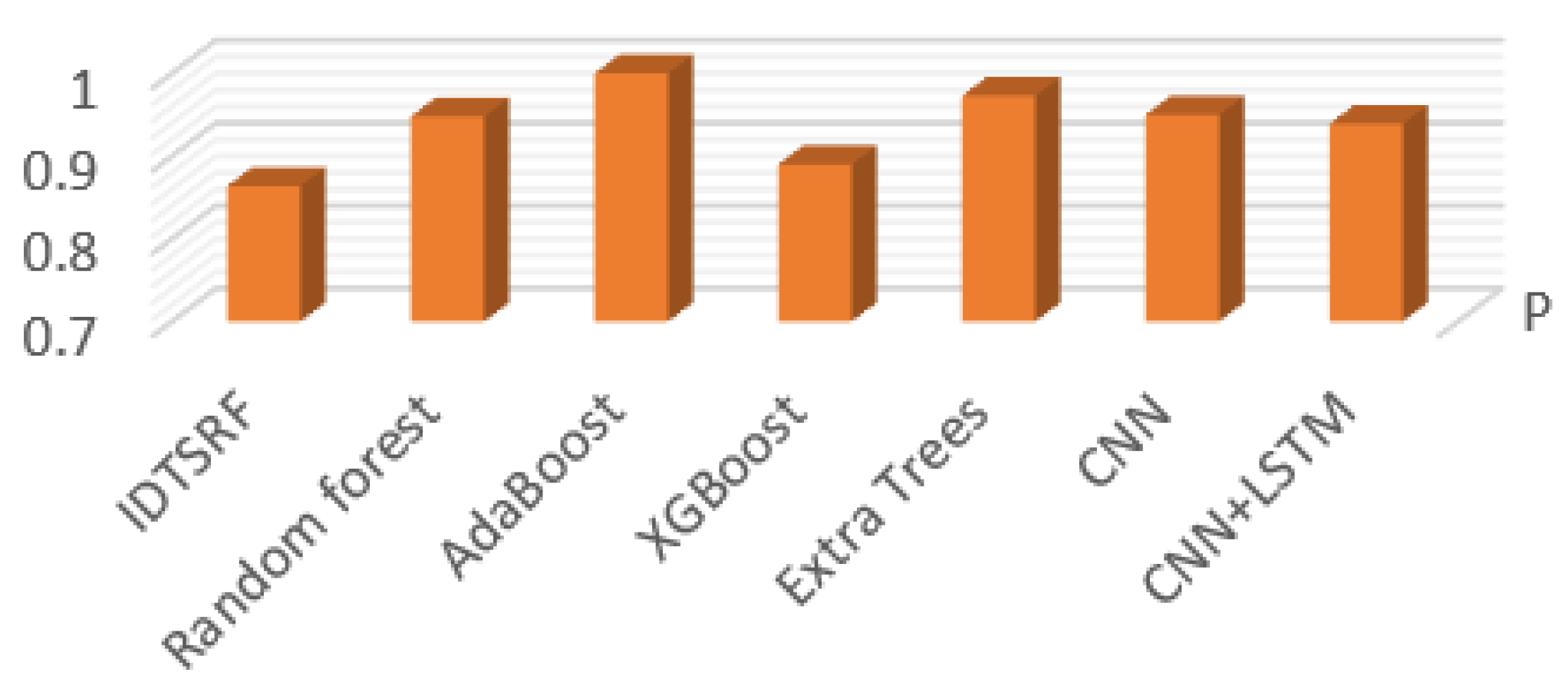
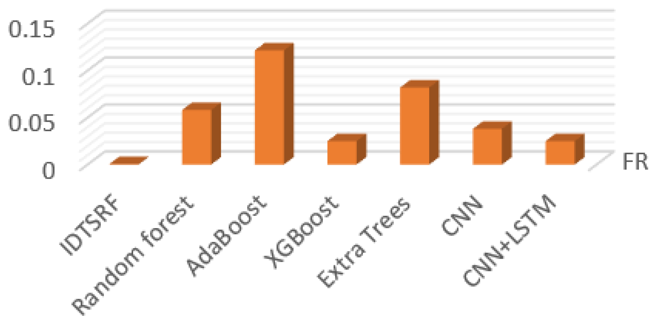
4.2. Algorithm Comparison Experiment

To further verify the nature of the IDTSRF, take the average value of 10 operation results (as shown in

Table 4. IDTSRF running results.

	FP	FR	P	R	F1
IDTSRF	0.1363	0.0006	0.8637	0.9994	0.9533
Random forest	0.052	0.0581	0.948	0.9419	0.9438
AdaBoost	0	0.1215	1	0.8785	0.9126
XGBoost	0.11	0.025	0.89	0.975	0.931
Extra Trees	0.027	0.082	0.973	0.918	0.945
CNN	0.05	0.038	0.95	0.962	0.9583
CNN + LSTM	0.061	0.025	0.939	0.975	0.957

) and compare it with the results of random forest, AdaBoost, XGBoost, extra trees, CNN, and CNN-LSTM, as shown in Figure 9, Figure 10, Figure 11, Figure 12 and Figure 13.

Due to the randomness of attribute selection, the results of each run are not exactly the same, as shown in Table 3. Intrusion detection pays more attention to the accuracy of correctly predicting intrusion behavior, so it focuses on the comparison between recall and other experimental results. The precision ratio indicates the proportion of the number of positive samples correctly classified by the model to the total number of positive samples. The overall precision value is between 80% and 93%, which is relatively volatile compared with the recall. The recall rate is basically stable, and the result is good, basically reaching 100%. Figure 9 and Figure 10 show the performance of all algorithms on recall and precision, respectively. It can be seen that the recall of the IDTSRF algorithm is obviously better than the other algorithms. Adaboost has the worst effect, and the recall is lower than 90%.

Figure 11, Figure 12 and Figure 13 show the comparison of bad debt rate, false negative rate, and the F1 values of different algorithms. Among them, the bad debt rate represents the proportion of the number of positive samples of model error classification in the total number of positive samples, and the false negatives rate represents the proportion of the number of positive samples of model error classification in the total number of correct classification samples. F1 is a harmonic average based on the precision and recall, which can comprehensively describe the performance of the algorithm and so focuses on observing the F1 value. Since NSL-KDD focuses on recall, $F_{\gamma }$ is taken as the evaluation standard and $\gamma =1.5$ as the result shown in Figure 13. It can be seen from the comparison that the F-value of the IDTSRF algorithm is basically the same as that of CNN and CNN-LSTM and is superior to other algorithms.

5. Conclusions

In this paper, we use the attribute measurement method based on decision boundary entropy to calculate the importance of attributes, increase the probability that attributes of the importance of attributes are selected, and randomly select a certain number of attributes in the positive domain, negative domain, and boundary domain through three decision-making ideas to obtain attribute subsets, train decision trees separately, and finally integrate random forests. On the one hand, this method takes into account the impact of attribute importance on classification results. On the other hand, we use the idea of ensemble learning to select subsets to train the base classifier and finally integrate to obtain the random forest model. The experimental results show that the algorithm in this paper is superior to random forest, AdaBoost, XGBoost, and extra forest in recall ratio and F1 value, and is basically the same as CNN and CNN-LSTM, which proves the effectiveness of the algorithm in this paper. Future work will further improve the precision of the algorithm in this paper. Considering the characteristics of the intrusion detection dataset, we will select three branches of data, and consider using the idea of three branches of decision-making to select and integrate the constructed base classifier, so as to improve the accuracy and diversity of integrated learning, thus improving the recall and precision of intrusion detection.

References

1. Yange, T.S.; Onyekware, O.; Abdulmuminu, Y.M. A Data Analytics System for Network Intrusion Detection Using Decision Tree. J. Comput. Sci. Appl. 2020, 8, 21–29. [Google Scholar]
2. Hassan, E.; Saleh, M.; Ahmed, A. Network Intrusion Detection Approach using Machine Learning Based on Decision Tree Algorithm. J. Eng. Appl. Sci. 2020, 7, 1. [Google Scholar] [CrossRef]
3. Bhati, B.S.; Rai, C.S. Analysis of Support Vector Machine-based Intrusion Detection Techniques. Arab. J. Sci. Eng. 2020, 45, 2371–2383. [Google Scholar] [CrossRef]
4. Shi, Q.; Kang, J.; Wang, R.; Yi, H.; Lin, Y.; Wang, J. A Framework of Intrusion Detection System based on Bayesian Network in IoT. Int. J. Perform. Eng. 2018, 14, 2280–2288. [Google Scholar] [CrossRef] [Green Version]
5. Prasath, M.K.; Perumal, B. A meta-heuristic Bayesian network classification for intrusion detection. Int. J. Netw. Manag. 2019, 29, e2047. [Google Scholar] [CrossRef]
6. Xu, G. Research on K-Nearest Neighbor High Speed Matching Algorithm in Network Intrusion Detection. Netinfo Secur. 2020, 20, 71–80. [Google Scholar]
7. Chao, D.; Gang, Z.; Liu, Y.; Zhang, D.L. The detection of network intrusion based on improved AdaBoost algorithm. J. Sichuan Univ. (Nat. Sci.Ed.) 2015, 52, 1225–1229. [Google Scholar]
8. Zhang, K.; Liao, G. Network intrusion detection method based on improving Bagging-SVM integration diversity. J. Northeast. Norm. Univ. (Nat. Sci.Ed.) 2020, 52, 53–59. [Google Scholar]
9. Li, B.; Zhang, Y. Research on Self-adaptive Intrusion Detection Based on Semi-Supervised Ensemble Learning. Electr. Autom. 2021, 43, 101–104. [Google Scholar]
10. Jiang, F.; Zhang, Y.Q.; Du, J.W.; Liu, G.Z.; Sui, Y.F. Approximate Reducts-based Ensemble Learning Algorithm and Its Application in Intrusion Detection. J. Beijing Univ. Technol. 2016, 42, 877–885. [Google Scholar]
11. Xia, J.M.; Li, C.; Tan, L.; Zhou, G. Improved Random Forest Classifier Network Intrusion Detection Method. Comput. Eng. Des. 2019, 40, 2146–2150. [Google Scholar]
12. Zhang, L.; Zhang, J.; Sang, Y. Intrusion Detection Algorithm Based on Random Forest and Artificial Immunity. Computer Engineering 2020, 46, 146–152. [Google Scholar]
13. Qiao, J.; Li, J.; Chen, C.; Chen, Y.; Lv, Y. Network Intrusion Detection Method Based on Random Forest. Comput. Eng. Appl. 2020, 56, 82–88. [Google Scholar]
14. Qiao, N.; Li, Z.; Zhao, G. Intrusion Detection Model of Internet of Things Based on XGBoost-RF. J. Chin. Comput. Syst. 2022, 43, 152–158. [Google Scholar]
15. Liang, B.; Wang, L.; Liu, Y. Attribute Reduction Based On Improved Information Entropy. J. Intell. Fuzzy Syst. 2019, 36, 709–718. [Google Scholar] [CrossRef]
16. Ayşegül, A.U.; Murat, D. Generalized Textural Rough Sets: Rough Set Models Over Two Universes. Inf. Sci. 2020, 521, 398–421. [Google Scholar]
17. Zhang, P.; Li, T.; Wang, G.; Luo, C.; Chen, H.; Zhang, J.; Wang, D.; Yu, Z. Multi-Source Information Fusion Based On Rough Set Theory: A Review. Inf. Fusion 2021, 68, 85–117. [Google Scholar] [CrossRef]
18. An, S.; Hu, Q.; Wang, C. Probability granular distance-based fuzzy rough set model. Appl. Soft Comput. 2021, 102, 107064. [Google Scholar] [CrossRef]
19. Han, S.E. Topological Properties of Locally Finite Covering Rough Sets And K-Topological Rough Set Structures. Soft Comput. 2021, 25, 6865–6877. [Google Scholar] [CrossRef]
20. Liu, J.; Bai, M.; Jiang, N.; Yu, D. A novel measure of attribute significance with complexity weight. Appl. Soft Comput. 2019, 82, 105543. [Google Scholar] [CrossRef]
21. Yao, Y. Three-Way Decision: An Interpretation of Rules in Rough Set Theory; Rough Sets and Knowledge Technology Springer: Berlin/Heidelberg, Germany, 2009. [Google Scholar]
22. Yao, Y. Three-way decisions with probabilistic rough sets. Inf. Sci. Int. J. 2010, 180, 341–353. [Google Scholar] [CrossRef]
23. Yao, Y. The superiority of three-way decisions in probabilistic rough set models. Inf. Sci. 2011, 181, 1080–1096. [Google Scholar] [CrossRef]
24. Rajadurai, H.; Gandhi, U.D. Naive Bayes and deep learning model for wireless intrusion detection systems. Int. J. Eng. Syst. Model. Simul. 2021, 12, 111–119. [Google Scholar] [CrossRef]
25. Xu, J.; Han, D.; Li, K.C.; Jiang, H. A K-means algorithm based on characteristics of density applied to network intrusion detection. Comput. Sci. Inf. Syst. 2020, 17, 665–687. [Google Scholar] [CrossRef]
26. Liu, J.; Liu, P.; Pei, S.; Tian, C. Design and Implementation of Network Anomaly Detection System Based on Association Rules. Cyber Secur. Data Gov. 2020, 39, 14–22. [Google Scholar] [CrossRef]
27. Jia, W.; Zhang, F.; Tong, B.; Wan, C. Application of Self-Organizing Mapping Neural Network in Intrusion Detection. Comput. Eng. Appl. 2009, 45, 115–117. [Google Scholar]
28. Sohn, I. Deep belief network based intrusion detection techniques: A survey. Expert Syst. Appl. 2021, 167, 114170. [Google Scholar] [CrossRef]
29. Wang, H.; Cao, Z.; Hong, B. A network intrusion detection system based on convolutional Neural Network. J. Intell. Fuzzy Syst. 2020, 38, 7623–7637. [Google Scholar] [CrossRef]
30. Sun, X. Intrusion Detection Method Based on Recurrent Neural Network. Master’s Thesis, Tianjin University, Tianjin, China, 2020. [Google Scholar] [CrossRef]
31. Rodríguez, J.J.; Kuncheva, L.I.; Alonso, C.J. Rotation forest: A new classifier ensemble method. IEEE Trans. Pattern Anal. Mach. Intell. 2006, 28, 1619–1630. [Google Scholar] [CrossRef]
32. Yulianto, A.; Sukarno, P.; Suwastika, N.A. Improving AdaBoost-based Intrusion Detection System (IDS) Performance on CIC IDS 2017 Dataset. J. Phys. Conf. Ser. 2019, 1192, 012018. [Google Scholar] [CrossRef]
33. Dhaliwal, S.S.; Nahid, A.A.; Abbas, R. Effective Intrusion Detection System Using XGBoost. Information 2018, 9, 149. [Google Scholar] [CrossRef]
34. Resende, P.A.A.; Drummond, A.C. A Survey of Random Forest Based Methods for Intrusion Detection Systems. ACM Comput. Surv. (CSUR) 2018, 51, 1–36. [Google Scholar] [CrossRef]
35. Wang, L.; Gu, C. Overview of Machine Learning Methods for Intrusion Detection. J. Shanghai Univ. Electr. Power 2021, 37, 591–596. [Google Scholar]
36. Yang, C.; Zhang, Q.; Zhao, F. Hierarchical Three-Way Decisions with Intuitionistic Fuzzy Numbers in Multi-Granularity Spaces. IEEE Access 2019, 7, 24362–24375. [Google Scholar] [CrossRef]
37. Wu, Q.; Huang, S. Intrusion Detection Algorithm Combining Convolutional Neural Network and Three-Branch Decision. Comput. Eng. Appl. 2022, 58, 119–127. [Google Scholar]
38. Du, X.; Li, Y. Intrusion Detection Algorithm Based on Deep Belief Network and Three Branch Decision. J. Nanjing Univ. (Nat. Sci.) 2021, 57, 272–278. [Google Scholar]
39. Zhang, S.; Li, Y. Intrusion Detection Method Based on Denoising Autoencoder and Three-way Decisions. Comput. Sci. 2021, 48, 345–351. [Google Scholar]
40. Hassan, M.; Butt, M.A.; Zaman, M. An Ensemble Random Forest Algorithm for Privacy Preserving Distributed Medical Data Mining. Int. J. E-Health Med. Commun. (IJEHMC) 2021, 12, 23. [Google Scholar] [CrossRef]
41. Zong, F.; Zeng, M.; He, Z.; Yuan, Y. Bus-Car Mode Identification: Traffic Condition–Based Random-Forests Method. J. Transp.Eng. Part A Syst. 2020, 146, 04020113. [Google Scholar] [CrossRef]
42. Zhang, P.; Jin, Y.F.; Yin, Z.Y.; Yang, Y. Random Forest based artificial intelligent model for predicting failure envelopes of caisson foundations in sand. Appl. Ocean. Res. 2020, 101, 102223. [Google Scholar] [CrossRef]
43. Zhang, C.; Ren, J.; Liu, F.; Li, X.; Liu, S. Three-way selection Random Forest algorithm based on decision boundary entropy. Appl. Intell. 2022, 52, 13384–13397. [Google Scholar] [CrossRef]
44. Bamakan SM, H.; Amiri, B.; Mirzabagheri, M.; Shi, Y. A New Intrusion Detection Approach using PSO based Multiple Criteria Linear Programming. Procedia Comput. Sci. 2015, 55, 231–237. [Google Scholar]
45. Shi, Y.; Tian, Y.; Kou, G.; Peng, Y.; Li, J. Optimization Based Data Mining: Theory and Applications: Theory and Applications; Springer: Berlin/Heidelberg, Germany, 2011. [Google Scholar]
46. Aghdam, M.H.; Kabiri, P. Feature Selection for Intrusion Detection System Using Ant Colony Optimization. Int. J. Netw. Secur. 2016, 18, 420–432. [Google Scholar]
47. Jiang, F.; Yu, X.; Du, J.; Gong, D.; Zhang, Y.; Peng, Y. Ensemble learning based on approximate reducts and bootstrap sampling. Inf. Sci. 2021, 547, 797–813. [Google Scholar] [CrossRef]
48. Meng, Q.; Zheng, S.; Cai, Y. Deep Learning SDN Intrusion Detection Scheme Based on TW-Pooling. J. Adv. Comput. Intell. Intell. Inform. 2019, 23, 396–401. [Google Scholar] [CrossRef]
Figure 1. Intrusion detection algorithms.
Mathematics 10 04460 g001
Figure 2. Flowchart of intrusion detection based on machine learning.
Mathematics 10 04460 g002
Figure 3. State diagram.
Mathematics 10 04460 g003
Figure 4. Random forest model diagram.
Mathematics 10 04460 g004
Figure 5. IDTSRF Model.
Mathematics 10 04460 g005
Figure 6. Precision change graph.
Mathematics 10 04460 g006
Figure 7. Recall variation chart.
Mathematics 10 04460 g007
Figure 8. Changes in precision and recall.
Mathematics 10 04460 g008
Figure 9. R Comparison chart.
Mathematics 10 04460 g009
Figure 10. P Comparison chart.
Mathematics 10 04460 g010
Figure 11. FP Comparison chart.
Mathematics 10 04460 g011
Figure 12. FR Comparison chart.
Mathematics 10 04460 g012
Figure 13. F1 Comparison chart.
Mathematics 10 04460 g013