
Recovery of Inhomogeneity from Output Boundary Data

1
Department of Mathematics, Cinvestav, Campus Querétaro, Libramiento Norponiente #2000, Fracc. Real de Juriquilla, Querétaro 76230, Mexico
2
Faculty of Engineering, Cerro de las Campanas s/n, col. Las Campanas Querétaro, Autonomous University of Queretaro, Querétaro 76010, Mexico
3
Department of Mathematics, Faculty of Science, Mersin University, 33343 Mersin, Turkey
*
Author to whom correspondence should be addressed.
Mathematics 2022, 10(22), 4349; https://doi.org/10.3390/math10224349
Submission received: 25 September 2022
/
Revised: 13 November 2022
/
Accepted: 17 November 2022
/
Published: 19 November 2022
(This article belongs to the Special Issue Analytical and Computational Methods in Differential Equations, Special Functions, Transmutations and Integral Transforms)
Abstract
:We consider the Sturm–Liouville equation on a finite interval with a real-valued integrable potential and propose a method for solving the following general inverse problem. We recover the potential from a given set of the output boundary values of a solution satisfying some known initial conditions for a set of values of the spectral parameter. Special cases of this problem include the recovery of the potential from the Weyl function, the inverse two-spectra Sturm–Liouville problem, as well as the recovery of the potential from the output boundary values of a plane wave that interacted with the potential. The method is based on the special Neumann series of Bessel functions representations for solutions of Sturm–Liouville equations. With their aid, the problem is reduced to the classical inverse Sturm–Liouville problem of recovering the potential from two spectra, which is solved again with the help of the same representations. The overall approach leads to an efficient numerical algorithm for solving the inverse problem. Its numerical efficiency is illustrated by several examples.
Keywords:
Sturm–Liouville equation; inverse problem; Weyl function; Neumann series of Bessel functions; numerical solution of inverse problemMSC:
34A55; 34B24; 34A25; 42C10; 65L091. Introduction
Let be real valued. Consider the one-dimensional Schrödinger equation
where is a spectral parameter, and is finite. Let be a solution of (1), satisfying some prescribed initial conditions at the origin
where and are some known functions that are not identical zeros.
In the present work, we propose a method for solving the following inverse problem.
Problem 1.
Given
for a number of values of , find .
This problem is of practical importance. For example, consider the following model. A plane wave , , incoming from , interacts with the potential (i.e., solves (1) for ) and is measured at the output, i.e., at the point for a number of frequencies , . The potential is to be recovered from these output boundary data. Thus, we have
and we need to recover , of course, approximately.
Note that is a Jost solution for the potential extended by zero from the segment onto the whole axis. Therefore, the problem consists in recovering the potential from its Jost solution measured at the interface point at several frequencies .
As another example, consider the problem of the recovery of the potential from the Weyl function given at a number of points. By we denote the Weyl solution of (1), which satisfies (1) as well as the boundary conditions
If is not a Neumann–Dirichlet eigenvalue of (1), the solution exists and is unique. By , we denote the Weyl function . Then, one of the frequently studied inverse Sturm–Liouville problems (see, e.g., [1,2,3,4,5]) consists in recovering from the Weyl function (given at a number of points). In other words, we have
From these data, the potential needs to be recovered.
Moreover, the classical two-spectra inverse problem (see, for example, [6,7,8,9]) is also a special case of Problem 1. Indeed, let be the eigenvalues of the Sturm–Liouville problem for (1) with the boundary conditions
while are the eigenvalues of the Sturm–Liouville problem for (1) with the conditions
That is, is an eigenfunction of the problem (1) and (5) when and of the problem (1) and (6) when . The set of can be chosen in the form of (here, in fact, the order does not matter). The set of data is
for all , because for all , the solution being an eigenfunction of (1) and (5) or (1) and (6) satisfies the homogeneous Dirichlet condition at . Thus, the inverse two-spectra problem is a special case of Problem 1.
The Problem 1 of recovering from the data
is generally not uniquely solvable even when the set of points is infinite. For example, when all are such that belongs to the Dirichlet–Dirichlet spectrum of (1), the knowledge of is not sufficient for recovering . In general, the characterization of such infinite sets of and of the rest of the data, for which the stated inverse problem is uniquely solvable, is a subtle matter (we refer to [5] for some results in this direction). In the present work, we restrict ourselves to the assumption that for a given infinite set of data of the form (8), the inverse problem is uniquely solvable, and we develop a method for its approximate solution. The overall approach is based on several recent results and ideas.
First of all, we use the Neumann series of Bessel functions (NSBF) representations for solutions of (1) obtained in [10]. They possess important properties, which make them especially convenient for dealing with problems, both direct and inverse, which require considering the spectral parameter admitting a large range of values. In particular, the remainders of the partial sums of the NSBF representations admit estimates independent of . Roughly speaking, the partial sums approximate the exact solutions equally well for small and for large values of . Moreover, the whole information on the potential is contained already in the first coefficient of the NSBF representation; so, for recovering , it is sufficient to compute the first coefficient alone. Behind these and some other remarkable features of the NSBF representations there stands the fact that they are obtained by expanding into a Fourier–Legendre series the integral kernel of the transmutation (transformation) operator. For the theory of transmutation operators, we refer to [11,12,13].
Second, we develop further the idea proposed in [14,15], which can be formulated as follows. An inverse problem can be efficiently solved by converting the input data into the computed values of the coefficients from the NSBF representations at the endpoint of the interval. This leads to the possibility of computing two different spectra for (1). The knowledge of two spectra and of the NSBF coefficients at the endpoint gives us the possibility of computing the first NSBF coefficient on the whole segment , which is sufficient for recovering .
The input data of the inverse problem can be of different nature. For example, in [14] they were the spectral data of the spectral problem on a quantum graph, while in [15] the input data were several first eigenvalues from two spectra for (1). In the present work, we show how the endpoint values of a solution of (1), which satisfies some given initial conditions, serve for recovering the potential , following the scheme described above.
In Section 2, we introduce the NSBF representations together with their basic properties. In Section 3, we develop the method for solving Problem 1. In Section 4, we summarize it in the form of an algorithm ready for implementation. In Section 5, we give several illustrations of its numerical performance. Finally, Section 6 contains some concluding remarks.
2. Preliminaries
By and we denote the solutions of the equation
satisfying the initial conditions
The main tool used in the present work is the series representations obtained in [10] for the solutions and of (9).
Theorem 1
([10]). The solutions and admit the following series representations
where stands for the spherical Bessel function of order k (see, e.g., [16]). The coefficients and can be calculated following a simple recurrent integration procedure (see [10]), starting with
For every , the series converges pointwise. For every , the series converges uniformly on any compact set of the complex plane of the variable ρ, and the remainders of their partial sums admit estimates independent of .
This last feature of the series representations (the independence of the bounds for the remainders of ) is a direct consequence of the fact that the representations are obtained by expanding the integral kernels of the transmutation operators (for their theory, we refer to [11,12,13]) into Fourier–Legendre series (see [10]). It is of crucial importance for what follows. In particular, it means that for
and
the estimates hold
for all , where is a positive function tending to zero when . That is, roughly speaking, the approximate solutions and approximate the exact ones equally well for small and for large values of . This is especially convenient when considering direct and inverse spectral problems. Moreover, for a fixed z, the numbers rapidly decrease as , (see, e.g., [16] [(9.1.62)]). Hence, the convergence rate of the series for any fixed is, in fact, exponential. More detailed estimates for the series remainders depending on the regularity of the potential can be found in [10].
Note that formulas (12) indicate that the potential can be recovered from the first coefficients of the series (10) or (11). We have
and
Note that the square roots of the Dirichlet–Dirichlet eigenvalues coincide with the zeros of the function :
while the square roots of the Neumann–Dirichlet eigenvalues coincide with zeros of the function :
3. Solution of Problem 1
From the very beginning, we assume that the set of the numbers , for which we dispose of the data (8), is finite. Thus, the problem consists in recovering approximately the potential from the data
where in general and the other data are complex numbers.
3.1. Computation of Coefficients and
In the first step, we use the data (16) to compute a number of the coefficients and from (10) and (11) evaluated at the endpoint . For this, let us substitute (10) and (11) into (2). We have
for all . Note that if , from (10) and (11), we have and , and (17) takes the form
Choosing such that , we consider the system of linear algebraic equations obtained from (17) by truncating the infinite sums,
for . Note that here and below we do not look to deal with square systems of equations. In computations, a least-squares solution of an overdetermined system (provided by Matlab, which we used for computations in this work) gives very satisfactory results and allows one to make use of all available data, while keeping the number of coefficients relatively small (in practice, or 5 may be sufficient).
Solving (18) gives us approximate values of the coefficients and . Here, we come to the problem of converting the knowledge of the coefficients from (10) and (11) evaluated at the endpoint of the interval into the information on on the whole interval.
The knowledge of the coefficients and allows us to compute the functions and for any value of . Due to the estimates in (13), we know that the accuracy of the approximation of the exact solutions and by these approximate ones does not deteriorate for large values of . So, in fact, we deal with the problem of converting the knowledge of the solutions or more generally of characteristic functions of two Sturm–Liouville problems for (9) at the endpoint into the information on on the whole interval. This problem naturally arises in the framework of different methods for solving inverse Sturm–Liouville problems. For example, in [17] (see also [18]), this problem was approached via an iterative algorithm based on the use of properties of the corresponding transmutation operator. In the present work, we apply another approach, which extends the one proposed in [14,15], and consists in converting the knowledge of and into an auxiliary inverse problem for (9) consisting in the recovery of from one spectrum and a sequence of corresponding multiplier constants. We formulate this problem in the next subsection and show how the knowledge of and allows us to reduce the inverse problem to that auxiliary inverse problem.
3.2. One Spectrum and Multiplier Constants Inverse Problem
Let be the eigenvalues of (9) with the Neumann-Dirichlet boundary conditions
Denote by a solution of (9) satisfying the initial conditions at :
for all . Hence, for , the solution is also an eigenfunction of (9) and (19). Hence, there exist the multiplier constants , , such that
The auxiliary inverse problem can be formulated as follows.
Problem 2.
Given the Neumann–Dirichlet spectrum of (9) and the multiplier constants , find .
A method for solving the problems of this type was proposed in [19]. Here, we develop the approach proposed in [14,15], where it was applied to slightly different situations. However, first, we show that the knowledge of the coefficients and can be used to reduce the original inverse Problem 1 to Problem 2.
As pointed out above, the knowledge of the coefficients and allows us to compute the approximate solutions and for any value of . This means that, in particular, we can compute zeros of these two functions. The following result establishes their proximity to zeros of the exact solutions and .
Theorem 2.
For any , there exists such that all zeros of the functions and are approximated by corresponding zeros of the functions and , respectively, with errors uniformly bounded by ε, and , have no other zeros.
Proof.
Since the zeros of and coincide with the square roots of the Neumann–Dirichlet and Dirichlet–Dirichlet eigenvalues of (9), the zeros of and for a sufficiently large N give us the approximate values of these singular numbers. We denote the Dirichlet–Dirichlet eigenvalues of (9) as . Thus, computing the zeros of and , we obtain the approximate numbers and . So, we reduce Problem 1 to a two-spectra inverse problem.
Analogously to solution (11), the solution admits the series representation
where are corresponding coefficients, analogous to from (11). The multiplier constants can be easily calculated by recalling that . Thus,
where we take into account that the spherical Bessel functions of odd order are odd functions. The coefficients are computed with the aid of the singular numbers as follows. Since the functions , are the Dirichlet–Dirichlet eigenfunctions of (9), we have that ; hence,
This leads to a system of linear algebraic equations for computing the coefficients , which has the form
where is the number of computed singular numbers , . Now, having computed , we compute the multiplier constants from (22), where is the number of the computed singular numbers .
Next, we use Equation (20) to construct a system of linear algebraic equations for the coefficients and . Indeed, Equation (20) can be written in the form
We have as many of these equations as the Neumann–Dirichlet singular numbers computed. For computational purposes, we choose some natural number —the number of the coefficients and to be computed. More precisely, we choose a sufficiently dense set of points , and at every , we consider the equations
Solving this system of equations, we find and consequently at a sufficiently dense set of points of the interval . Finally, with the aid of (14), we compute .
4. Algorithm
Given the data (8), the algorithm of the solution of Problem 1 consists of the following steps.
- (1)
- Choose , such that , and compute the sets of coefficients and from (18).
- (2)
- Compute a number of zeros of the function , which approximate the Neumann–Dirichlet singular numbers, and a number of zeros of the function , which approximate the Dirichlet–Dirichlet singular numbers of .
- (3)
- Compute the coefficients from (23).
- (4)
- Compute the constants from (22).
- (5)
- Choose , such that , and a number of points . For each , solve (24) to find .
- (6)
- Compute from (14).
In the last step, we used the spline approximation for and differentiated it twice.
5. Numerical Examples
The proposed method can be implemented directly using an available numeric computing environment. All the computations were performed in Matlab 2017 on an Intel i7-7600U (Intel, Santa Clara, CA, USA) equipped laptop computer. We start with the simplest example of a constant potential, which is convenient for illustrating the performance of the algorithm in each step by comparing the results with the exact ones.
Example 1.
Consider the potential , , where is a constant. Let us consider the problem of recovering from the Weyl function, that is, from the data of the form (4). For the constant potential, we have
We chose 15 points distributed uniformly on and computed . That gave us the data (4). For numerical implementation of the algorithm we chose and , and with the coefficients and computed in the first step, we computed 40 Neumann–Dirichlet singular numbers and 39 Dirichlet–Dirichlet singular numbers .
In Table 1, some of the exact and computed (marked by tilde) singular numbers are provided together with the absolute error. Similar results were obtained for the Dirichlet–Dirichlet singular numbers, see Table 2.
Thus, the partial sums and with the corresponding coefficients computed from (18) allow us to compute both spectra with a remarkable accuracy. We emphasize that many more of the higher indices eigenvalues can be computed with a non-deteriorating accuracy, though usually several dozens are sufficient for recovering the potential.
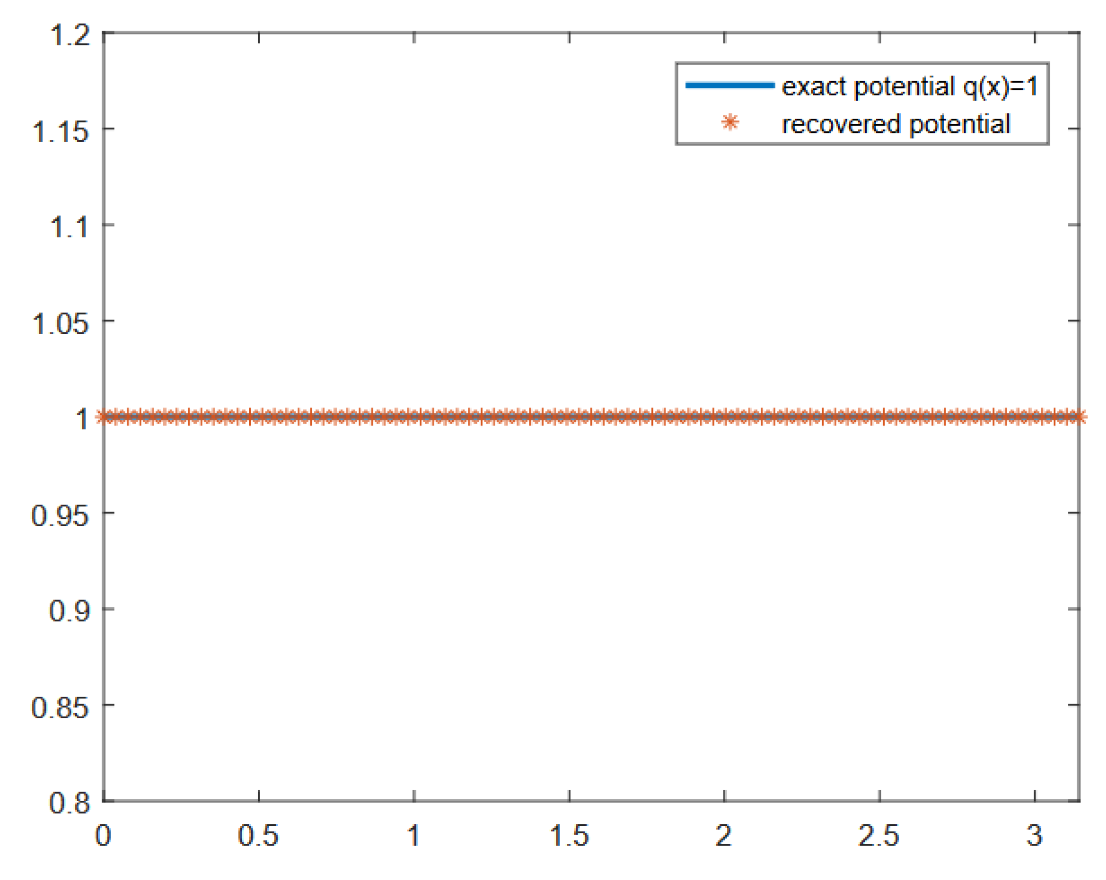
Next, following the algorithm, we computed the coefficients from (23) and from (22). In step 5, we chose , though the results were similar for an chosen between and . In Figure 1, the recovered potential is depicted; the maximum absolute error was equal to .
Choosing more points and a larger number N leads to more accurate results. For example, with 25 points distributed uniformly on the same interval and , the maximum absolute error of the recovered potential was . Remarkably, the maximum absolute error of the first 40 Neumann–Dirichlet singular numbers computed was and for the Dirichlet–Dirichlet singular numbers. The numerical solution of the inverse incident plane wave problem of recovering the potential from the data (3) with the same choice of the points and N led to similarly accurate results: the maximum absolute error of the recovered potential was .
For the same constant potential, we considered the inverse problem with the data corresponding to two spectra (7) with and . For the first ten eigenpairs given and , the potential was recovered with the maximum absolute error , while for five eigenpairs given and , the maximum absolute error was .
Example 2.
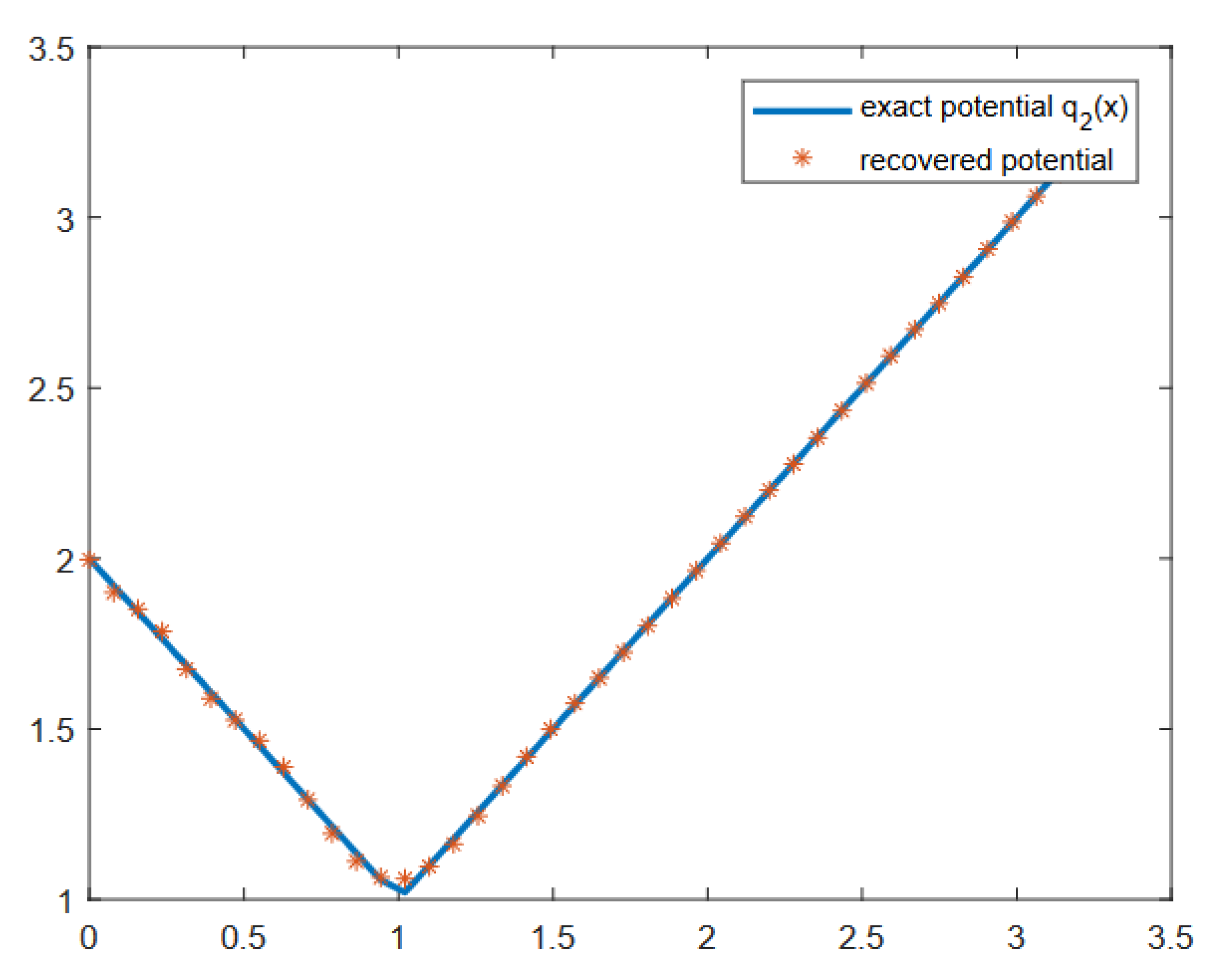
Consider the inverse incident plane wave problem for the non-smooth and continuous potential
We chose 25 points distributed uniformly on the segment in the complex plane and the corresponding data of the type (3). In Figure 2, the result of the solution of the inverse problem is presented. The number of the coefficients was chosen as ten (i.e., ). The maximum absolute error (attained at ) was .
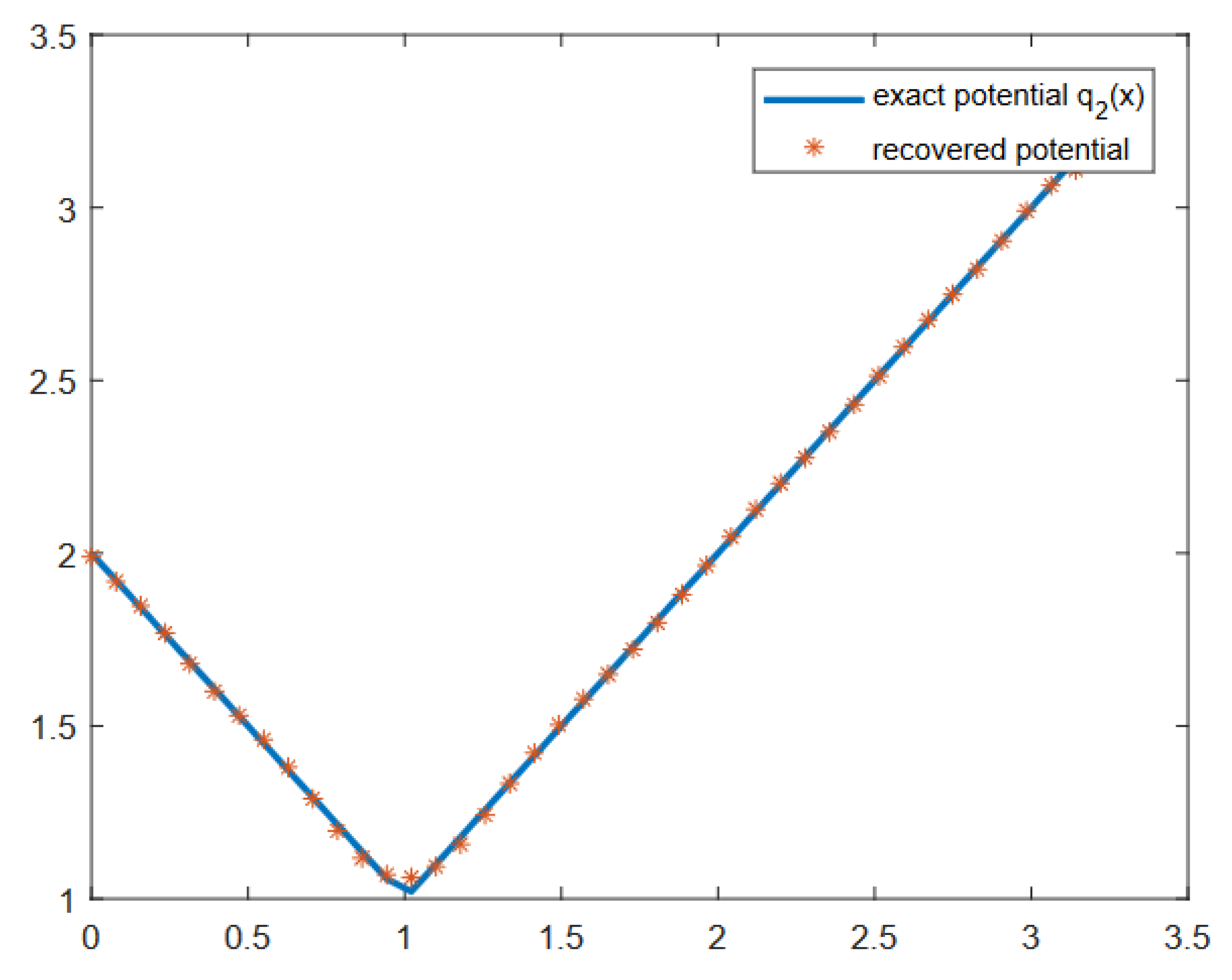
For the same potential and points , we generated the data corresponding to and , which led to similar results (Figure 3).
6. Conclusions
A simple method for solving a general inverse problem for the Sturm–Liouville equation, consisting in recovering the potential from the output boundary values of a solution satisfying certain prescribed initial conditions, was developed. The data of the problem were converted into the knowledge of the coefficients of the Neumann series of Bessel functions, representations of two linearly independent solutions evaluated at the endpoint, which allowed us to reduce the problem to a two-spectra inverse Sturm–Liouville problem. This problem was solved by reducing it to a system of linear algebraic equations from which the first coefficient of the Neumann series of Bessel functions representation was found, which led to the recovery of the potential.
The method is simple, direct, accurate, and applicable to a large variety of inverse problems. Its performance was illustrated by numerical examples.
Author Contributions
Conceptualization, V.V.K.; Methodology, V.V.K.; Software, V.V.K. and K.V.K.; Formal analysis, V.V.K.; Investigation, V.V.K., K.V.K. and F.A.Ç.; Writing—original draft, V.V.K.; Writing—review and editing, K.V.K. and F.A.Ç.; Supervision, V.V.K.; Project administration, V.V.K.; Funding acquisition, V.V.K. All authors have read and agreed to the published version of the manuscript.
Funding
The research was supported by CONACYT, Mexico, via the project 284470 and partially performed at the Regional Mathematical Center of the Southern Federal University with the support of the Ministry of Science and Higher Education of Russia, agreement 075-02-2022-893.
Institutional Review Board Statement
Not applicable.
Informed Consent Statement
Not applicable.
Data Availability Statement
The data that support the findings of this study are available upon reasonable request.
Conflicts of Interest
The authors declare no competing interests.
References
- Bondarenko, N.P. Inverse Sturm—Liouville problem with analytical functions in the boundary condition. Open Math. 2020, 18, 512–528. [Google Scholar] [CrossRef]
- Bondarenko, N.P. Solvability and stability of the inverse Sturm–Liouville problem with analytical functions in the boundary condition. Math. Methods Appl. Sci. 2020, 43, 7009–7021. [Google Scholar] [CrossRef]
- Gesztesy, F.; del Rio, R.; Simon, B. Inverse spectral analysis with partial information on the potential, III. Updating boundary conditions. Int. Math. Res. Notices 1997, 15, 751–758. [Google Scholar]
- Horváth, M. Inverse spectral problems and closed exponential systems. Ann. Math. 2005, 162, 885–918. [Google Scholar] [CrossRef] [Green Version]
- Yurko, V.A. Introduction to the Theory of Inverse Spectral Problems; Fizmatlit: Moscow, Russia, 2007. [Google Scholar]
- Gao, Q.; Cheng, X.; Huang, Z. On a boundary value method for computing Sturm–Liouville potentials from two spectra. Int. J. Comput. Math. 2014, 91, 490–513. [Google Scholar] [CrossRef]
- Guliyev, N.J. On two-spectra inverse problems. Proc. Am. Math. Soc. 2020, 148, 4491–4502. [Google Scholar] [CrossRef]
- Kammanee, A.; Böckmann, C. Boundary value method for inverse Sturm–Liouville problems. Appl. Math. Comput. 2009, 214, 342–352. [Google Scholar] [CrossRef]
- Savchuk, A.M.; Shkalikov, A.A. Inverse problem for Sturm–Liouville operators with distribution potentials: Reconstruction from two spectra. Russ. J. Math. Phys. 2005, 12, 507–514. [Google Scholar]
- Kravchenko, V.V.; Navarro, L.J.; Torba, S.M. Representation of solutions to the one-dimensional Schrödinger equation in terms of Neumann series of Bessel functions. Appl. Math. Comput. 2017, 314, 173–192. [Google Scholar] [CrossRef] [Green Version]
- Levitan, B.M. Inverse Sturm–Liouville Problems; VSP: Zeist, The Netherlands, 1987. [Google Scholar]
- Marchenko, V.A. Sturm–Liouville Operators and Applications: Revised Edition; AMS Chelsea Publishing: New York, NY, USA, 2011. [Google Scholar]
- Shishkina, E.L.; Sitnik, S.M. Transmutations, Singular and Fractional Differential Equations with Applications to Mathematical Physics; Elsevier: Amsterdam, The Netherlands, 2020. [Google Scholar]
- Avdonin, S.; Kravchenko, V.V. Method for solving inverse spectral problems on quantum star graphs. J. Inverse-Ill-Pose P. 2022; in press. [Google Scholar]
- Kravchenko, V.V. Spectrum completion and inverse Sturm-Liouville problems. Math. Method Appl. Sci. 2022, in press. [Google Scholar] [CrossRef]
- Abramovitz, M.; Stegun, I.A. Handbook of Mathematical Functions; Unites States Department of Commerce: New York, NY, USA, 1972. [Google Scholar]
- Rundell, W.; Sacks, P.E. Reconstruction techniques for classical inverse Sturm–Liouville problems. Math. Comput. 1992, 58, 161–183. [Google Scholar] [CrossRef]
- Chadan, K.; Colton, D.; Päivxaxrinta, L.; Rundell, W. An Introduction to Inverse Scattering and Inverse Spectral Problems; SIAM: Philadelphia, PA, USA, 1997. [Google Scholar]
- Brown, B.M.; Samko, V.S.; Knowles, I.W.; Marletta, M. Inverse spectral problem for the Sturm—Liouville equation. Inverse Probl. 2003, 19, 235–252. [Google Scholar] [CrossRef]
- Kravchenko, V.V.; Torba, S.M. Analytic approximation of transmutation operators and applications to highly accurate solution of spectral problems. J. Comput. Appl. Math. 2015, 275, 1–26. [Google Scholar] [CrossRef]
Figure 1.
Potential from Example 1 recovered from the Weyl function given at 15 points and with N = 4.
Figure 1.
Potential from Example 1 recovered from the Weyl function given at 15 points and with N = 4.

Figure 2.
Potential recovered from the data of type (3) with 25 points distributed uniformly on the segment in the complex plane and .
Figure 2.
Potential recovered from the data of type (3) with 25 points distributed uniformly on the segment in the complex plane and .

Figure 3.
Potential recovered from the data (8) with 25 points distributed uniformly on the segment in the complex plane , and , corresponding to , and .
Figure 3.
Potential recovered from the data (8) with 25 points distributed uniformly on the segment in the complex plane , and , corresponding to , and .

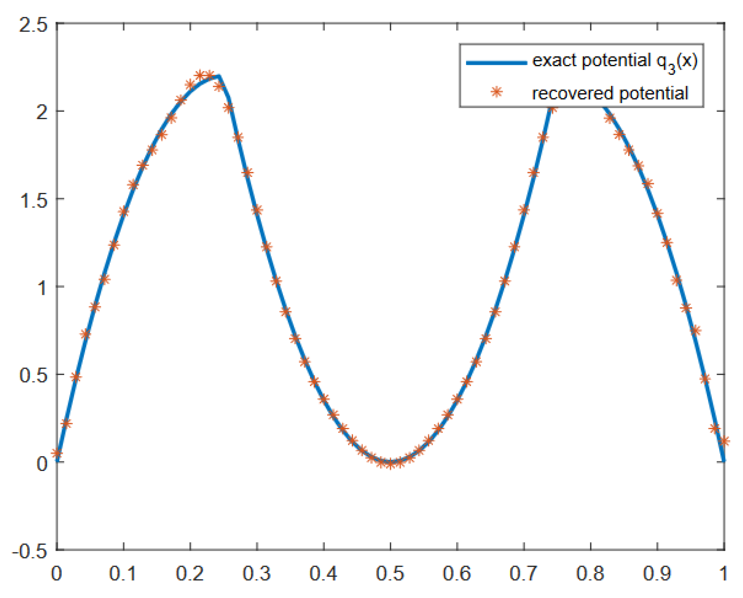
Figure 4.
Potential recovered from the data of type (3) given at 60 points distributed uniformly on the segment and .
Figure 4.
Potential recovered from the data of type (3) given at 60 points distributed uniformly on the segment and .


Table 1.
Neumann–Dirichlet singular numbers of q from Example 1.
| j | |||
|---|---|---|---|
| 0 | |||
| 10 | |||
| 20 | |||
| 39 |
Table 2.
Dirichlet–Dirichlet singular numbers of q from Example 1.
| j | |||
|---|---|---|---|
| 1 | |||
| 11 | |||
| 21 | |||
| 39 |
Publisher’s Note: MDPI stays neutral with regard to jurisdictional claims in published maps and institutional affiliations. |
© 2022 by the authors. Licensee MDPI, Basel, Switzerland. This article is an open access article distributed under the terms and conditions of the Creative Commons Attribution (CC BY) license (https://creativecommons.org/licenses/by/4.0/).
Share and Cite
MDPI and ACS Style
Kravchenko, V.V.; Khmelnytskaya, K.V.; Çetinkaya, F.A. Recovery of Inhomogeneity from Output Boundary Data. Mathematics 2022, 10, 4349. https://doi.org/10.3390/math10224349
AMA Style
Kravchenko VV, Khmelnytskaya KV, Çetinkaya FA. Recovery of Inhomogeneity from Output Boundary Data. Mathematics. 2022; 10(22):4349. https://doi.org/10.3390/math10224349
Chicago/Turabian StyleKravchenko, Vladislav V., Kira V. Khmelnytskaya, and Fatma Ayça Çetinkaya. 2022. "Recovery of Inhomogeneity from Output Boundary Data" Mathematics 10, no. 22: 4349. https://doi.org/10.3390/math10224349
Note that from the first issue of 2016, this journal uses article numbers instead of page numbers. See further details here.