Risk Diffusion and Control under Uncertain Information Based on Hypernetwork

Abstract

During the height of the COVID-19 epidemic, production lagged and enterprises could not deliver goods on time, which will bring considerable risks to the supply chain system. Modeling risk diffusion in supply chain networks is important for prediction and control. To study the influence of uncertain information on risk diffusion in a dynamic network, this paper constructs a dynamic evolution model based on a hypernetwork to study risk diffusion and control under uncertain information. First, a dynamic evolution model is constructed to represent the network topology, which includes the addition of links, rewiring of links, entry of nodes, and the exit of outdated nodes that obey the aging principle. Then, the risk diffusion scale is discussed with the Microscopic Markovian Chain Approach (MMCA), and the risk threshold is analyzed. Finally, the consistency of Monte Carlo (MC) simulation and MMCA is verified by MATLAB, and the influence of each parameter on the risk diffusion scale and risk threshold is tested. The results show that reducing the cooperation and production during the risk period, declining the attenuation factor, enhancing the work efficiency of the official media, and increasing the probability of the exit of outdated nodes in the supply chain networks will increase the risk threshold and restrain the risk diffusion.

1. Introduction

Retail, manufacturing, and consumer goods companies face challenges in managing their profit margins due to the ongoing impact of the COVID-19 and supply chain issues. To produce high-quality products that meet market demand and obtain maximum benefits, enterprises continue to strengthen ties with others. The increase in cooperation will lead to network structure being more complex. The complexity of the supply chain network and the uncertainty of characteristics will cause potential losses in terms of efficiency and effectiveness target values [1]. Furthermore, COVID-19 delayed the resumption of production of manufacturing industry. Inadequate personnel, blocked logistics, and lack of funds, resulting in a decline in production capacity. Some enterprises’ demand for raw materials has reduced, which has impacted the front-end enterprises of the supply chain. Capacity supply is insufficient, and the back end of the supply chain suffers from the shortage of raw materials. The risks brought by above events are aggravated under the influence of economic globalization. Therefore, the study of risk diffusion in the supply chain network has become an important part of the field of propagation dynamics.

In recent years, most dynamic research has focused on single-layer networks, such as risk diffusion in supply chain networks [2], information dissemination [3] in social networks, epidemic spreading [4], etc. He et al. proposed a competitive information dissemination macro model to study the intrinsic relationship between the competition mechanism among different types of information and the rules of node state transition and information propagation evolution [5]. Garg et al. used the discrete-time model of the SIR model to analyze COVID-19, and project the upcoming behavior of the pandemic [6]. However, complex systems in the reality are composed of multiple subsystems. Thus, scholars begin to consider using multiplex networks as a basic tool for researching dynamics [7,8], studying the risk diffusion caused by untimely supply under the warning information [9].

Actually, there is often a time separation between the evolution of the network structure and the dynamical propagation process in the existing multiplex networks research. Based on the WS small-world network, Qian et al. have built a credit risk contagion model with the influence of information dissemination to analyze the influence factors [10]. Zhang et al. studied information diffusion under public crises in BA scale-free networks [11]. Most of the research is focused on static networks. However, the actual network structure will change with time. For example, the diffusion of green information on online social networks is accompanied by the addition of new nodes, linking of old nodes, and rewiring of links [12].

In addition, research on risk diffusion in supply chain networks has focused on complex networks [8,9]. With the increase in cooperation, an enterprise may have multiple cooperation projects, each cooperation has multiple participants. The complex cooperation relationship makes the complex network described by ordinary graphs no longer suitable for current research. The hypernetwork was proposed by Denning in 1985 [13], and then Ernesto Estrada proposed a hypergraph-based hypernetwork [14]. The emergence of hypernetwork is beneficial to describing the complex network topology and evolution process in reality. It can be used to describe the characteristics and evolution mode of the supply chain system [15], and describe the non-uniform evolution of social networks [16]. Hypernetwork theory also be used in the field of dynamics, building propagation models to describe information propagation in dynamic social hypernetworks [17].

Based on the above considerations, the paper studies the risk diffusion process in the supply chain network based on the two-layer dynamic hypernetwork model and puts forward effective suggestions on how to control the risk diffusion caused by untimely supply. The main novelty and contributions of this paper are as follows:

• First, a dynamic evolution model of the supply chain network is constructed based on a hypernetwork, in which the exit of nodes in the system follows the aging principle.
• Second, consider the influence of official media on the virtual information layer, and study the risk diffusion mechanism under uncertain information.
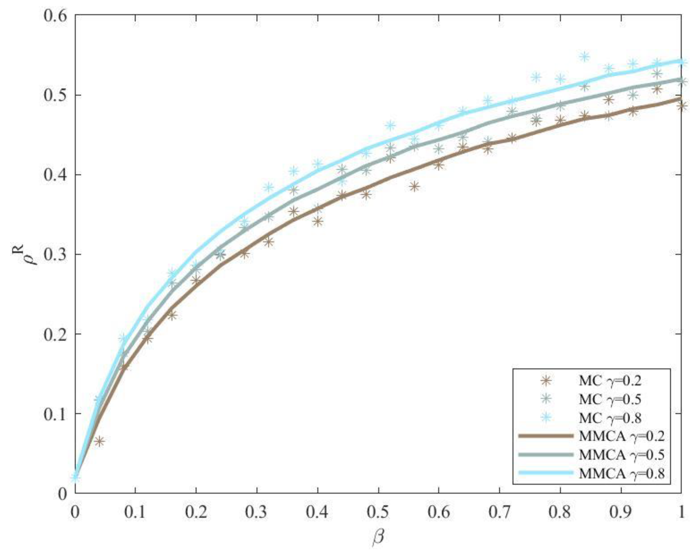
• Third, the effectiveness of MMCA is verified by MC simulation, and the influence of various parameters on risk diffusion is tested via MMCA.

The paper is organized as follows: Section 2 introduces the dynamic evolution model and the UBU-SEIR model; Section 3 uses MMCA for theoretical analysis; Section 4 verifies the effectiveness of MMCA through MATLAB and tests the influence of each parameter in turn; Section 5 summarizes the research in the paper and proposes future research directions.

2. Model Description

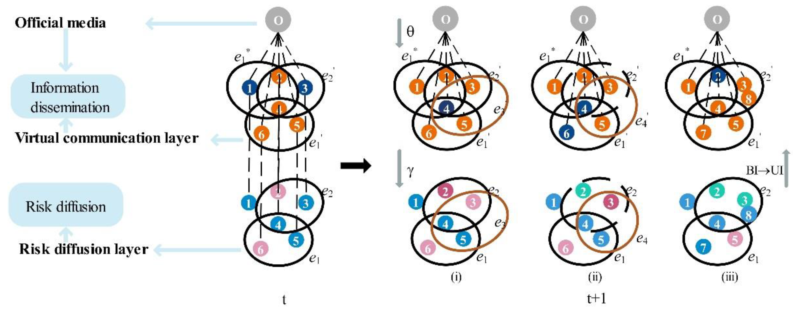
2.1. Dynamic Evolution Model

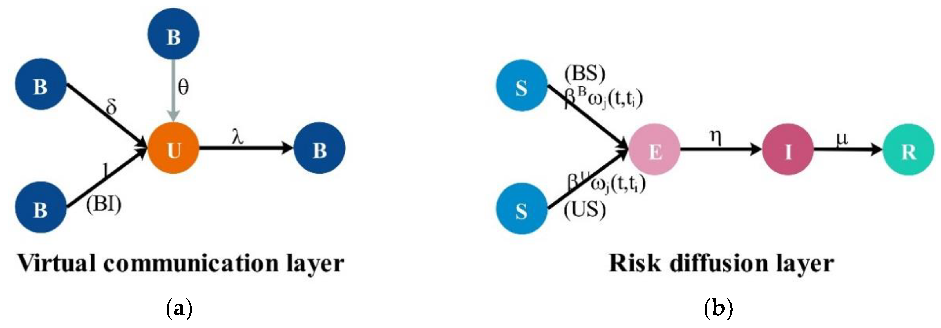
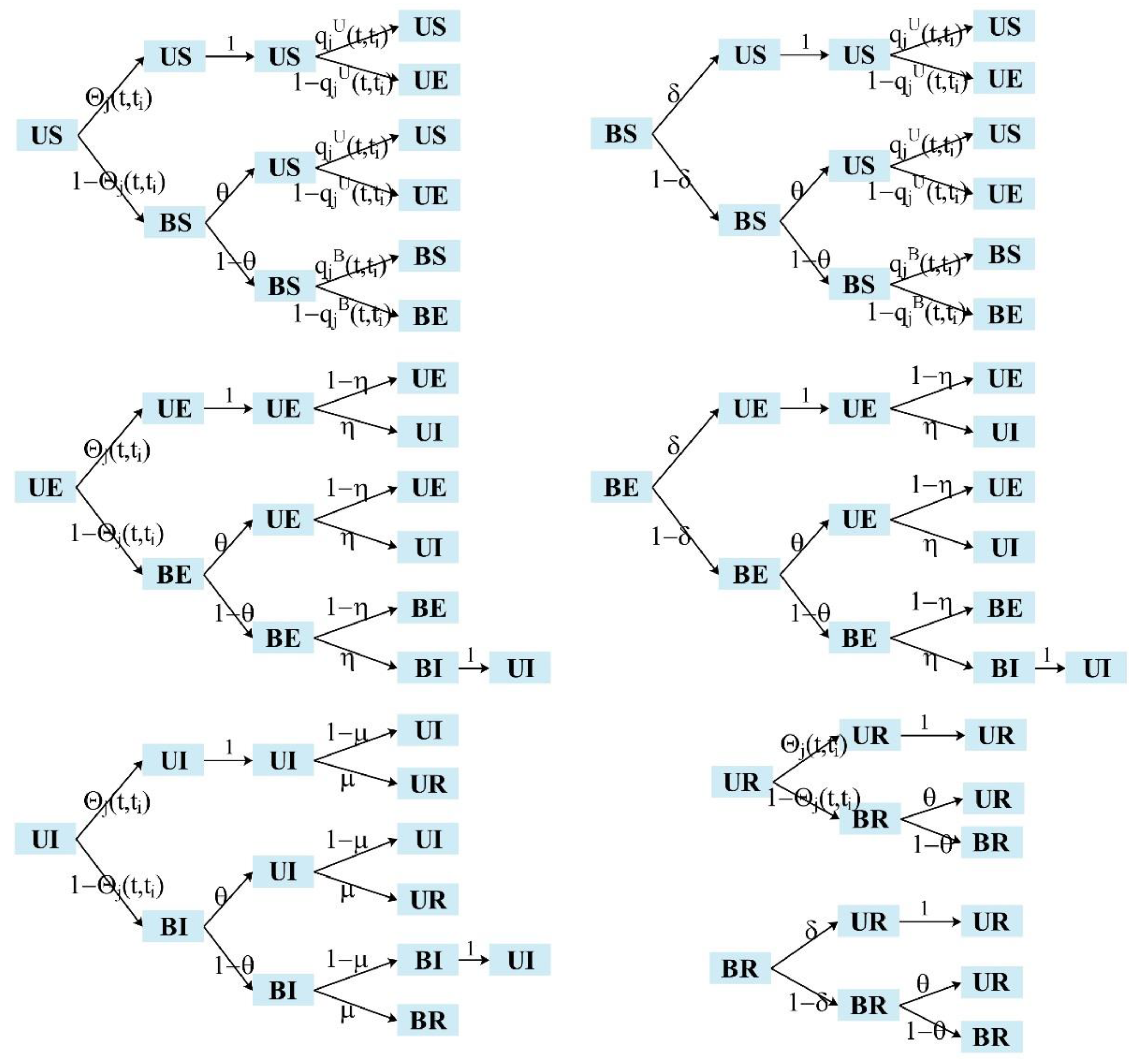
The mathematical definition of a hypernetwork:

The set of nodes $V=\left\{v_1,v_2,\cdots ,v_n\right\}$ is a finite set, and hyperedge $E_i=\left\{v_{i1},v_{i2},\cdots ,v_{i{l}_i}\right\}$$\left(v_{iy}\in V,y=1,2,\cdots l_i.\right)$ is a non-empty subset of $V$, the set of hyperedges $E^h=\left\{E_1,E_2,\cdots ,E_m\right\}$ is a family of non-empty subsets of $V$. The pair $H=\left(V,E^h\right)$ is known as a hypergraph. Hypernetworks are networks described by hypergraphs, which are above and beyond networks represented by ordinary graphs. In this paper, a two-layer hypernetwork is constructed to study the risk diffusion and control under uncertain information. The upper layer is the social network, and the lower layer is the supply chain network. In the supply chain network described by hypernetwork, nodes represent enterprises, node set $V=\left\{v_1,v_2,\cdots ,v_n\right\}$ represents all enterprises in the system; hyperedge $E_i$ represents the cooperation formed by some enterprises $v_{i1},v_{i2},\cdots ,v_{i{l}_i}$, and hyperedge sets $E^h$ represent all cooperation $E_1,E_2,\cdots ,E_m$ existing in the system. Social networks described by hypernetworks are similar [16].

With the development of the economy, enterprise cooperation in the supply chain has expanded from the initial small scope to the global [18,19]. Each enterprise forms new cooperation according to market demand to obtain maximum benefits, and the company will end the old cooperation and start new cooperation because of economic benefits when the contract expires. Besides, there will always be the entry of new enterprises and the exit of outdated enterprises in the market. The supply chain network considers three evolution processes based on the above: (i) establishing new cooperative relations with existing enterprises; (ii) replacing old ones with new partners and developing new cooperation; (iii) the entry of emerging enterprises and the exit of outdated enterprises in the market.

The size and link of the supply chain network will change as the nodes enter and exit. Furthermore, there is more and more cooperation in the context of economic globalization, an enterprise may have multiple cooperation, and multiple enterprises may gather because of benefits. Therefore, this paper describes the dynamic evolution process of the supply chain network with hypernetwork. Considering that the proportion of enterprises entering and leaving the system is not necessarily the same, assume nodes arrive at the system and leave the system accordance with a Poisson process with rates ${\lambda }_1$ and ${\lambda }_2({\lambda }_1\ge {\lambda }_2)$, respectively. The number of arrived nodes in each batch is $m_2$. The example of the dynamic network evolution process is shown in Figure 1, the meaning of parameters in the model is shown in

Table 1. The meaning of parameters.

Parameters	Meaning of the Parameters
$p$	Probability of adding hyperedges
$q$	Probability of rewiring hyperedges
$r$	Probability of adding nodes and removing outdated nodes
$m$	Number of hyperedges added (or rewired)
$m_1$	Number of outdated nodes removed
$m_2$	Number of new nodes added
$\delta$	Wakefulness rate
$\theta$	The rate at which official media publishes accurate information
$\eta$	Probability of transition from E-state to I-state

, and the evolution of the supply chain network can be summarized as the following dynamic mechanisms:

(1) Add $m$ hyperedges to the system with probability $p$. First, randomly select a node, and then form a hyperedge with $\alpha$ nodes selected according to Equation (1). This process is repeated $m$ times without overlapping.

$$W_j(t,t_i)=\frac{h_j(t,t_i)+1}{{\displaystyle \sum _{ij}\left(h_j(t,t_i)+1\right)}}.$$

(1)

Hyperdegree indicates the number of hyperedges containing a node. In this model, the larger the hyperdegree $h_j(t,t_i)$ is, the more hyperedges containing the $j$th node in the $i$th batch. This means that the node has a lot of cooperation and it will attract more nodes to cooperate with it, considering that well-known companies are more attractive for small business cooperation. The hyperdegree preferential attachment mechanism [20] as shown in Equation (1) is used to select nodes, where $h_j(t,t_i)$ denotes the hyperdegree of the $j$th node in the $i$th batch at time $t$. $W_j(t,t_i)$ represents the probability that the $j$th node in the $i$th batch is selected at time $t$.

(2) Rewire $m$ hyperedges with probability $q$. First, a node $i$ and a hyperedge $e_i$ containing it are chosen randomly, and then $e_i$ is replaced with $e_i^{″}$ which is composed of node $i$ and the other $\alpha$ nodes selected through Equation (1). This process is repeated $m$ times without overlapping. The hyperdegree of node $i$ has not changed, and the hyperdegree of other nodes may change.

(3) Add $m_2$ nodes and remove $m_1$ outdated nodes with probability $r$. Nothing lasts forever; they all have a certain lifespan. After a long time, the system will reach a saturation state, and enterprises in the early years will withdraw from the market because they do not meet the needs of contemporary development. Therefore, the selection of exit nodes follows the aging principle, i.e., outdated nodes that enter the system earlier are easier to exit.

One of the three dynamic processes must occur at each time step $t$ to ensure the dynamic evolution of the network, i.e., the event probability satisfies $p+q+r\equiv 1$. In a social network, nodes and hyperedges represent enterprises and social relationships, respectively. The dynamic evolution of the social network is consistent with the above-mentioned supply chain network since enterprise cooperation always be accompanied by information interaction. However, social networks are large in scale and number. There is also a random exchange of information among enterprises that are not cooperating. Hence, on the basis of the same network topology as the supply chain network, some hyperedges are added to represent the information exchange among non-cooperative enterprises.

2.2. UBU-SEIR Model

In fact, untimely production and supply will indeed affect the supply chain system. For example, affected by the COVID-19, the production restriction and stop of Vietnamese factories from July to September 2020 had a major shock on Nike and other manufacturing industries. Based on the research of Yin et al. [21], we study the risk diffusion process under uncertain information with hypernetwork. The uncertain information refers to the misleading information that affects the production cooperation, while the risk refers to the enterprises not being able to deliver goods on time due to untimely supply. In a two-layer multiplexing network, each node on one layer is mapped to the corresponding nodes on another layer, but the links among nodes in the upper layer may not exist in the lower layer.

Assume uncertain information spreads on the virtual communication layer via the UBU (Unbelieve-believe-Unbelieve) model. U-state means that the enterprise does not believe in uncertain information that will mislead cooperation, while a B-state enterprise does. In Figure 2a, the U-state enterprise will be informed uncertain information by B-state friends, and then enter the B-state with probability $\lambda$. The B-state enterprise will wake up from the misleading of uncertain information with rate $\delta$, and become a U-state that does not believe in uncertain information. The above information propagation process is at the individual level, while the clarification of the official media and the appearance of accurate information will inhibit the propagation of uncertain information. Considering a more realistic situation, we introduce the official media which is a node connected to each node in the virtual communication layer, it regularly transmits market-related information to all enterprises with rate $\theta$, so that the B-state enters the U-state.

The past research on risk diffusion in supply chain networks has used the SIR model [9], ignoring the existence of potential risks [22] which is a transitional state between susceptible and infected. Assume the risk spreads on the risk diffusion layer via the SEIR (Susceptible-Exposed-Infected-Recovered) model [23]. Infected enterprises include E-state and I-state, where E-state means an enterprise is infected by risks and unaware of the risk, while I-state means an enterprise has been deeply involved in risk. Both E-state and I-state enterprises will infect S-state enterprises with risk. Considering the node with the greater the hyperdegree has more cooperation, and the probability ${\omega }_j(t,t_i)$ of being infected by risk is the greater. In Figure 2b, S-state enterprises first enter E-state with probability $\beta$ after being infected by risk with probability ${\omega }_j(t,t_i)$, then E-state enterprises enter I-state with rate $\eta$, and finally I-state enterprises enter R-state with rate $\mu$. R-state enterprises will have relevant experiences after recovering, thus they will not be infected by the risk again.

$${\omega }_j(t,t_i)=\frac{h_j(t,t_i)}{Max(h(t))}.$$

(2)

The greater the hyperdegree of a node is, the more cooperation it has, and the greater the probability that it be infected by risks. Therefore, ${\omega }_j(t,t_i)$ is used to represent the probability that the $j$th node in the $i$th batch is infected by risk, where, $h_j(t,t_i)$ represents the hyperdegree of the $j$th node in the $i$th batch, and $Max(h(t))$ represents the maximum hyperdegree in the network at time $t$.

Uncertain information propagation and risk diffusion are two mutual influence processes. Risk diffusion will inhibit the propagation of uncertain information, while the uncertain information will accelerate the diffusion of risks in the supply chain network. Assume an enterprise infected by risk, it will realize the wrongness of information immediately and no longer believe, i.e., the BI-state individual will enter the UI state with probability 100%, thus the BI state is not considered here. Once an enterprise recovers from risk, it will lose vigilance and forget uncertain information. Because of the diversity of information, the recovered enterprise will again believe uncertain information. The BR state needs to be considered here. In addition, the probability ${\beta }^U$ of enterprises who do not believe in uncertain information entering the E-state is smaller than the probability ${\beta }^B({\beta }^B=\beta )$ of enterprises who believe entering the E-state. Therefore, the attenuation factor $\gamma (0\le \gamma \le 1)$ is introduced, such that ${\beta }^U=\gamma {\beta }^B=\gamma \beta$.

In summary, each node in the coupled dynamic network of social network and supply chain network will be in one of 7 states: US (Unbelieve and Susceptible), UE (Unbelieve and Exposed), UI (Unbelieve and Infected), UR (Unbelieve and Recovered), BS (Believe and Susceptible), BE (Believe and Exposed), BR (Believe and Recovered). Combining the descriptions of the dynamic evolution model and the UBU-SEIR model, the risk diffusion mechanism under the uncertain information based on the hypernetwork is shown in Figure 3.

3. Theoretical Analysis

The total node number of hypernetwork is $N(t)$, new hyperedge contains $\alpha +1$ nodes. The hyperdegree $h_j(t,t_i)$ is a continuous variable affected by the process (1)–(3) in Section 2.1, thus $h_j(t,t_i)$ satisfies the following three dynamic equations according to the continuous technique:

$$\frac{\partial h_j(t,t_i)}{\partial t}=pm({\lambda }_1-{\lambda }_2)\left[\frac{1}{N(t)}+\alpha \frac{h_j(t,t_i)+1}{{\displaystyle \sum _{ij}\left(h_j(t,t_i)+1\right)}}\right],$$

(3)

$$\frac{\partial h_j(t,t_i)}{\partial t}=qm({\lambda }_1-{\lambda }_2)\left[-\frac{1}{N(t)}+\alpha \frac{h_j(t,t_i)+1}{{\displaystyle \sum _{ij}\left(h_j(t,t_i)+1\right)}}\right],$$

(4)

$$\frac{\partial h_j(t,t_i)}{\partial t}=-r{\lambda }_2{m}_1\frac{t_{ij}{}^{-1}}{{\displaystyle \sum _{ij}{t}_{ij}{}^{-1}}}{h}_j(t,t_i),$$

(5)

where $t_{ij}$ represents the arrival time of the $j$th node in the $i$th batch to the system, which is used to select the exiting aging node. Equations (3)–(5) corresponds to the process (1)–(3) in Section 2.1.

Combining Equations (3)–(5), we can get

$$\begin{array}{cc}\hfill \frac{\partial h_j(t,t_i)}{\partial t}& =\frac{m({\lambda }_1-{\lambda }_2)}{N(t)}(p-q)+\alpha \frac{h_j(t,t_i)+1}{{\displaystyle \sum _{ij}\left(h_j(t,t_i)+1\right)}}m({\lambda }_1-{\lambda }_2)(p+q)\hfill \\ & -r{\lambda }_2{m}_1\frac{t_{ij}{}^{-1}}{{\displaystyle \sum _{ij}{t}_{ij}{}^{-1}}}{h}_j(t,t_i)\hfill \end{array}$$

(6)

For large $t$,

$$N(t)\approx \left({\lambda }_1-{\lambda }_2\right)t, {\displaystyle \sum _{ij}\left(h_j(t,t_i)+1\right)}\approx \left[mp(\alpha +1)+m_2-r{m}_1\right]\times E\left[N(t)\right].$$

(7)

Let $D=\underset{t\to \infty }{\lim }\frac{{\displaystyle \sum _{ij}{t}_{ij}{}^{-1}}}{N(t)}$, $G=\frac{D}{m_1}$, substituting Equation (7) into Equation (6), then

$$\begin{array}{cc}\hfill \frac{\partial h_j(t,t_i)}{\partial t}=& \frac{m({\lambda }_1-{\lambda }_2)}{({\lambda }_1-{\lambda }_2)t}(p-q)+\frac{\alpha m({\lambda }_1-{\lambda }_2)(p+q)}{\left[mp(\alpha +1)+m_2-r{m}_1\right]({\lambda }_1-{\lambda }_2)t}\left(h_j(t,t_i)+1\right)\hfill \\ & -r{\lambda }_2\frac{t_{ij}^{-1}}{({\lambda }_1-{\lambda }_2)tG}{h}_j(t,t_i)\hfill \\ & =\frac{1}{t}\left[m(p-q)+\left(\frac{\alpha m(p+q)}{mp(\alpha +1)+m_2-r{m}_1}-\frac{r{\lambda }_2{t}_{ij}{}^{-1}}{G({\lambda }_1-{\lambda }_2)}\right)h_j(t,t_i)\right.\hfill \\ & \left.+\frac{\alpha m(p+q)}{mp(\alpha +1)+m_2-r{m}_1}\right]\hfill \end{array}$$

(8)

For simplicity, let $J=m(p-q)$, $L=\frac{\alpha m(p+q)}{mp(\alpha +1)+m_2-r{m}_1}-\frac{r{\lambda }_2{t}_{ij}{}^{-1}}{G({\lambda }_1-{\lambda }_2)}$, $Q=\frac{\alpha m(p+q)}{mp(\alpha +1)+m_2-r{m}_1}$.

Then, we obtain

$$\frac{\partial h_j(t,t_i)}{\partial t}=\frac{1}{t}\left[J+L{h}_j(t,t_i)+Q\right].$$

(9)

By integrating the two sides, we can get

$${\left(\frac{t}{t_i}\right)}^L=\frac{J+L{h}_j(t,t_i)+Q}{J+L{h}_j(t_i,t_i)+Q}.$$

(10)

From the initial conditions, we know that the $j$th node in the $i$th batch arriving at the system at $t_i$ satisfies $h_j(t_i,t_i)=r$, solving Equation (10), we obtain

$$h_j(t,t_i)=\left(r+\frac{J+Q}{L}\right){\left(\frac{t}{t_i}\right)}^L-\frac{J+Q}{L}.$$

(11)

Then,

$$\omega \left(h_j(t,t_i)\right)=\frac{h_j(t,t_i)}{Max(h(t))}=\frac{\left(r+\frac{J+Q}{L}\right){\left(\frac{t}{t_i}\right)}^L-\frac{J+Q}{L}}{Max(h(t))}.$$

(12)

In the risk diffusion layer, if there is a link between the node $n_{ij}$ and $n_{zl}$, then $a_{ijzl}=1$, otherwise $a_{ijzl}=0$; if node $n_{ij}$ is connected to node $n_{zl}$ in the virtual communication layer, then $b_{ijzl}=1$, otherwise $b_{ijzl}=0$. Where $n_{ij}$ represents the $j$th node in the $i$th batch, $n_{zl}$ is similar to it. Each node $n_{ij}$ is in one of seven states at time $t$ with a certain probability, which is $P_j^{US}(t,t_i)$, $P_j^{BS}(t,t_i)$, $P_j^{UE}(t,t_i)$, $P_j^{BE}(t,t_i)$, $P_j^{UI}(t,t_i)$, $P_j^{UR}(t,t_i)$, $P_j^{BR}(t,t_i)$, respectively. Let ${\Theta }_j(t,t_i)$ denote the probability of node $n_{ij}$ does not receive uncertain information from neighbors when $n_{ij}$ was U-state, $q_j^U(t,t_i)$ denote the probability of node $n_{ij}$ is not infected by risk when $n_{ij}$ was in US-state, $q_j^B(t,t_i)$ denote the probability of node $n_{ij}$ is not infected by risk when $n_{ij}$ was in BS-state.

$${\Theta }_j(t,t_i)=\underset{z}{\Pi }\underset{l}{\Pi }\left[1-b_{ijzl}{P}_l^B(t,t_z)\lambda \right],$$

(13)

$$q_j^U(t,t_i)=\underset{z}{\Pi }\underset{l}{\Pi }\left[1-a_{ijzl}\left(P_l^E(t,t_z)+P_l^I(t,t_z)\right)\kappa {\omega }_j(t,t_i){\beta }^U\right],$$

(14)

$$q_j^B(t,t_i)=\underset{z}{\Pi }\underset{l}{\Pi }\left[1-a_{ijzl}\left(P_l^E(t,t_z)+P_l^I(t,t_z)\right)\kappa {\omega }_j(t,t_i){\beta }^B\right],$$

(15)

where $\kappa$ denotes the adjustment coefficient of ${\omega }_j(t,t_i)$, $\lambda$ denotes the probability of believing uncertain information, $\beta$ denotes the probability of transition from state S to state E, while $P_l^B(t,t_z)=P_l^{BS}(t,t_z)+P_l^{BE}(t,t_z)+P_l^{BR}(t,t_z)$, $P_l^I(t,t_z)=P_l^{UI}(t,t_z)$, $P_l^E(t,t_z)=P_l^{UE}(t,t_z)+P_l^{BE}(t,t_z)$.

Considering each time step is divided into three continuous processes: the propagation of uncertain information (UBU), the accurate information dissemination by official media, and the diffusion of risk (SEIR). As shown in Figure 4, we construct a state transition probability tree through Figure 2 and Equations (13)–(15) to represent the state transition between seven possible states.

MMCA is an approach for analyzing the spread of epidemics in the network [24,25], and it is also applicable to the diffusion of risks in the supply chain network [9]. Based on Figure 4, the Markov chain for representing state transition [26] is derived as follows:

$$P_j^{US}(t+1,t_i)=P_j^{US}(t,t_i)q_j^U(t,t_i)\left[{\Theta }_j(t,t_i)+\left(1-{\Theta }_j(t,t_i)\right)\theta \right]+P_j^{BS}(t,t_i)q_j^U(t,t_i)\left[\delta +(1-\delta )\theta \right],$$

(16)

$$P_j^{BS}(t+1,t_i)=P_j^{US}(t,t_i)\left(1-{\Theta }_j(t,t_i)\right)(1-\theta )q_j^B(t,t_i)+P_j^{BS}(t,t_i)(1-\delta )(1-\theta )q_j^B(t,t_i),$$

(17)

$$\begin{array}{cc}\hfill P_j^{UE}(t+1,t_i)=& \left[P_j^{US}(t,t_i)\left(1-q_j^U(t,t_i)\right)+P_j^{UE}(t,t_i)(1-\eta )\right]\left[{\Theta }_j(t,t_i)+\left(1-{\Theta }_j(t,t_i)\right)\theta \right],\hfill \\ & +P_j^{BS}(t,t_i)\left(1-q_j^U(t,t_i)\right)\left[\delta \right.\left.+(1-\delta )\theta \right]+P_j^{BE}(t,t_i)(1-\eta )\left[\delta +(1-\delta )\theta \right]\hfill \end{array}$$

(18)

$$\begin{array}{cc}\hfill P_j^{BE}(t+1,t_i)=& P_j^{US}(t,t_i)\left(1-{\Theta }_j(t,t_i)\right)(1-\theta )\left(1-q_j^B(t,t_i)\right)+P_j^{BS}(t,t_i)(1-\delta )(1-\theta )\left(1-q_j^B(t,t_i)\right),\hfill \\ & +P_j^{UE}(t,t_i)\left(1-{\Theta }_j(t,t_i)\right)(1-\theta )(1-\eta )+P_j^{BE}(t,t_i)(1-\delta )(1-\theta )(1-\eta )\hfill \end{array}$$

(19)

$$P_j^{UI}(t+1,t_i)=P_j^{UE}(t,t_i)\eta +P_j^{BE}(t,t_i)\eta +P_j^{UI}(t,t_i)(1-\mu ),$$

(20)

$$\begin{array}{cc}\hfill P_j^{UR}(t+1,t_i)=& P_j^{UI}(t,t_i)\left[{\Theta }_j(t,t_i)\mu +\left(1-{\Theta }_j(t,t_i)\right)\theta \mu \right]+P_j^{UR}(t,t_i)\left[{\Theta }_j(t,t_i)+\left(1-{\Theta }_j(t,t_i)\right)\theta \right],\hfill \\ & +P_j^{ER}(t,t_i)\left[\delta +(1-\delta )\theta \right]\hfill \end{array}$$

(21)

$$P_j^{BR}(t+1,t_i)=\left[\mu P_j^{UI}(t,t_i)+P_j^{UR}(t,t_i)\right]\left(1-{\Theta }_j(t,t_i)\right)(1-\theta )+P_j^{BR}(t,t_i)(1-\delta )(1-\theta ).$$

(22)

Obviously, the normalization condition

$$P_j^{US}(t,t_i)+P_j^{BS}(t,t_i)+P_j^{UE}(t,t_i)+P_j^{BE}(t,t_i)+P_j^{UI}(t,t_i)+P_j^{UR}(t,t_i)+P_j^{BR}(t,t_i)\equiv 1$$

(23)

holds at each time step.

Each state probability of each node reaches a steady state when $t\to \infty$, thus $P_j{(t+1,t_i)}_{t\to \infty }=P_j{(t,t_i)}_{t\to \infty }=P_{ij}$. The risk threshold is a key parameter of risk diffusion in the supply chain network. The probability of an enterprise infecting the risk approaches 0 when the risk is near the threshold. Assuming that the S-state enterprise first enters the E-state when it is infected by a risk, then $P_{ij}^E={\epsilon }_{ij}\ll 1$. Therefore, Equation (20) can be simplified to $P_{ij}^{UI}=\frac{\eta }{\mu }{\epsilon }_{ij}$, Equations (14) and (15) can be approximated as

$$q_j^U(t,t_i)\approx 1-{\displaystyle \sum _z{\displaystyle \sum _l{a}_{ijzl}\left(P_l^E(t,t_z)+P_l^I(t,t_z)\right)\kappa {\omega }_j(t,t_i){\beta }^U}}=1-\gamma \left(1+\frac{\eta }{\mu }\right){\xi }_{ij},$$

(24)

$$q_j^B(t,t_i)\approx 1-{\displaystyle \sum _z{\displaystyle \sum _l{a}_{ijzl}\left(P_l^E(t,t_z)+P_l^I(t,t_z)\right)\kappa {\omega }_j(t,t_i){\beta }^B}}=1-\left(1+\frac{\eta }{\mu }\right){\xi }_{ij},$$

(25)

where

$${\xi }_{ij}=\kappa {\omega }_j(t,t_i){\beta }^B{\displaystyle \sum _z{\displaystyle \sum _l{a}_{ijzl}{\epsilon }_{zl}}}.$$

(26)

In the steady state, adding Equations (18) and (19) can get

$$\begin{array}{cc}\hfill P_{ij}^E=& P_{ij}^{US}\left\{\left(1-q_{ij}^U\right)\left[{\Theta }_{ij}+\left(1-{\Theta }_{ij}\right)\theta \right]+\left(1-{\Theta }_{ij}\right)(1-\theta )\left(1-q_{ij}^B\right)\right\}\hfill \\ & +P_{ij}^{BS}\left\{\left(1-q_{ij}^U\right)\left[\delta +(1-\delta )\theta \right]+(1-\delta )(1-\theta )\left(1-q_{ij}^B\right)\right\}+P_{ij}^E(1-\eta )\hfill \end{array}$$

(27)

Next, substituting Equations (24) and (25) into Equation (27), we get

$$\begin{array}{cc}\hfill {\epsilon }_{ij}=& (1-\eta ){\epsilon }_{ij}+P_{ij}^{US}\left\{\gamma \left(1+\frac{\eta }{\mu }\right){\xi }_{ij}\left[{\Theta }_{ij}+\left(1-{\Theta }_{ij}\right)\theta \right]+\left(1-{\Theta }_{ij}\right)(1-\theta )\left(1+\frac{\eta }{\mu }\right){\xi }_{ij}\right\}\hfill \\ & +P_{ij}^{BS}\left\{\gamma \left(1+\frac{\eta }{\mu }\right){\xi }_{ij}\left[\delta +(1-\delta )\theta \right]+(1-\delta )(1-\theta )\left(1+\frac{\eta }{\mu }\right){\xi }_{ij}\right\}\hfill \end{array}$$

(28)

Around the risk threshold, $P_{ij}^{UE}\to 0$, $P_{ij}^{BE}\to 0$, $P_{ij}^{UI}\to 0$, $P_{ij}^{UR}\to 0$ and $P_{ij}^{BR}\to 0$, thus $P_{ij}^U=P_{ij}^{US}+P_{ij}^{UE}+P_{ij}^{UI}+P_{ij}^{UR}\approx P_{ij}^{US}$, $P_{ij}^B=P_{ij}^{BS}+P_{ij}^{BE}+P_{ij}^{BR}\approx P_{ij}^{BS}$, Equation (28) can be written as

$$\begin{array}{cc}\hfill {\epsilon }_{ij}=& (1-\eta ){\epsilon }_{ij}+\gamma \left(1+\frac{\eta }{\mu }\right){\xi }_{ij}\left\{P_{ij}^U\left[{\Theta }_{ij}+\left(1-{\Theta }_{ij}\right)\theta \right]+P_{ij}^B\left[\delta +(1-\delta )\theta \right]\right\}\hfill \\ & +\left(1+\frac{\eta }{\mu }\right){\xi }_{ij}\left[P_{ij}^U\left(1-{\Theta }_{ij}\right)(1-\theta )+P_{ij}^B(1-\delta )(1-\theta )\right]\hfill \end{array}$$

(29)

In the steady state, removing $O({\epsilon }_{ij})$ terms of Equations (16) and (17), we can get

$$P_{ij}^U=P_{ij}^U\left[{\Theta }_{ij}+\left(1-{\Theta }_{ij}\right)\theta \right]+P_{ij}^B\left[\delta +(1-\delta )\theta \right],$$

(30)

$$P_{ij}^B=P_{ij}^U\left(1-{\Theta }_{ij}\right)(1-\theta )+P_{ij}^B(1-\delta )(1-\theta ).$$

(31)

Substituting Equations (30) and (31) into Equation (29), then

$${\epsilon }_{ij}=(1-\eta ){\epsilon }_{ij}+\gamma \left(1+\frac{\eta }{\mu }\right){\xi }_{ij}{P}_{ij}^U+\left(1+\frac{\eta }{\mu }\right){\xi }_{ij}{P}_{ij}^B.$$

(32)

Considering Equation (26), Equation (32) can be further transformed into

$${\displaystyle \sum _{zl}\left[\left(\gamma P_{ij}^U+P_{ij}^B\right)\kappa {\omega }_{ij}{a}_{ijzl}-\frac{\mu \eta }{(\mu +\eta ){\beta }^B}{c}_{ijzl}\right]}{\epsilon }_{zl}=0.$$

(33)

Number the node $n_{ij}$ in the order of appearance, and $ij=1,2,\cdots N$, same for $zl$. $c_{ijzl}$ is an element of the identity matrix, i.e., if $ij=zl$, then $c_{ijzl}=1$, otherwise $c_{ijzl}=0$. The elements of matrix F are defined as $f_{ijzl}=\left(\gamma P_{ij}^U+P_{ij}^B\right)\kappa {\omega }_{ij}{a}_{ijzl}$, and ${\Lambda }_{\max }$ is the largest eigenvalue of matrix F. According to Equation (33), the risk threshold of the proposed model can be written as

$${\beta }_c^B=\frac{\mu \eta }{(\mu +\eta ){\Lambda }_{\max }},$$

(34)

where ${\beta }_c={\beta }_c^B$ is considered as the solution to the eigenvalue problem. It can be seen that the risk threshold is related to the network topology and model parameters through Equation (34). Next, we will verify the correctness of the above theoretical analysis by numerical simulation.

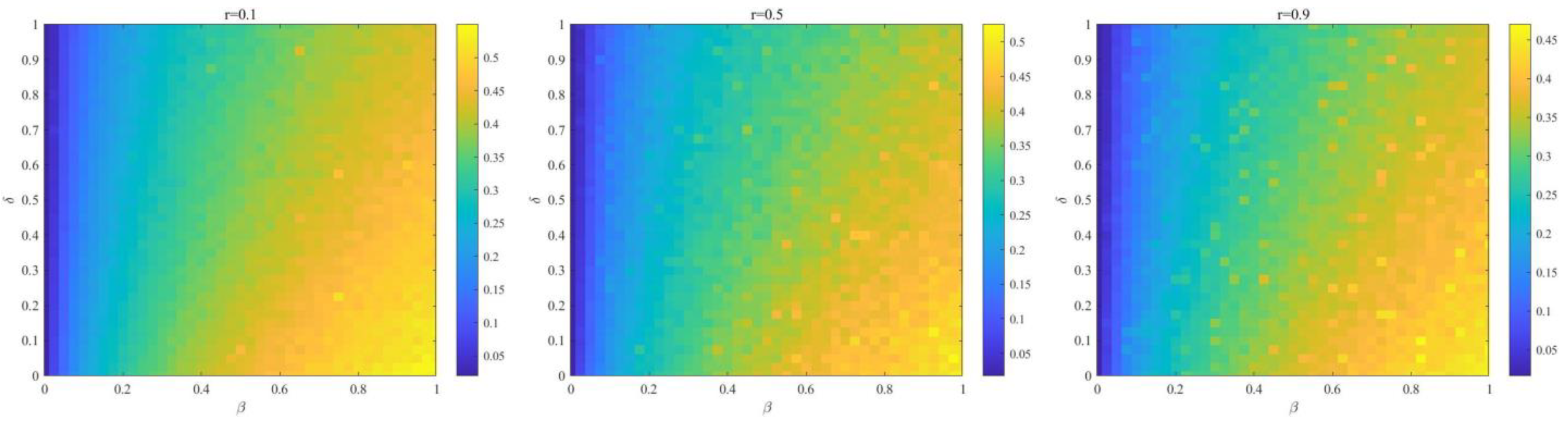
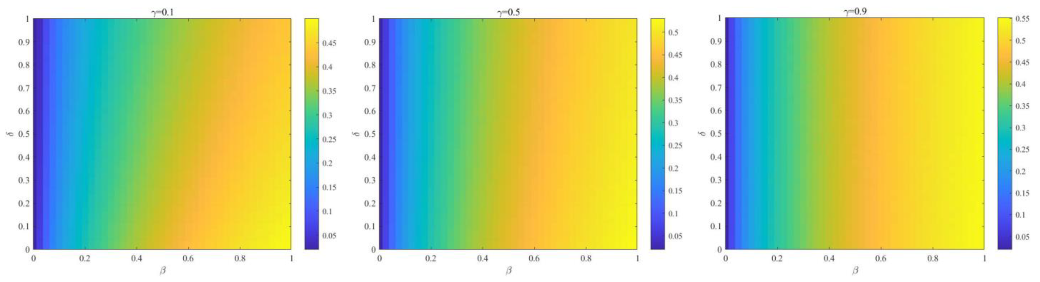
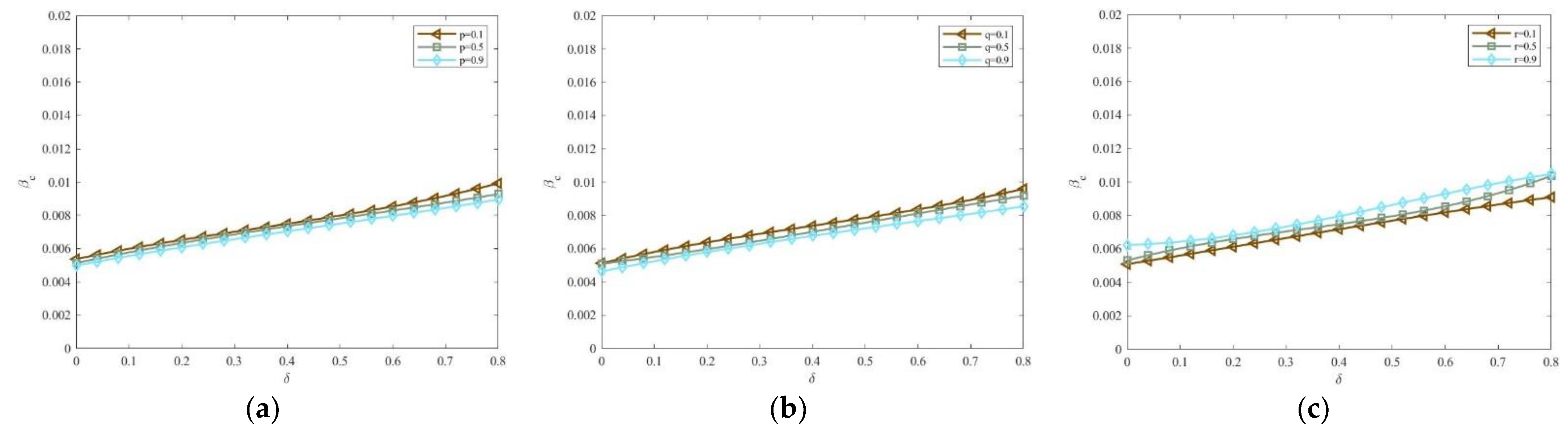
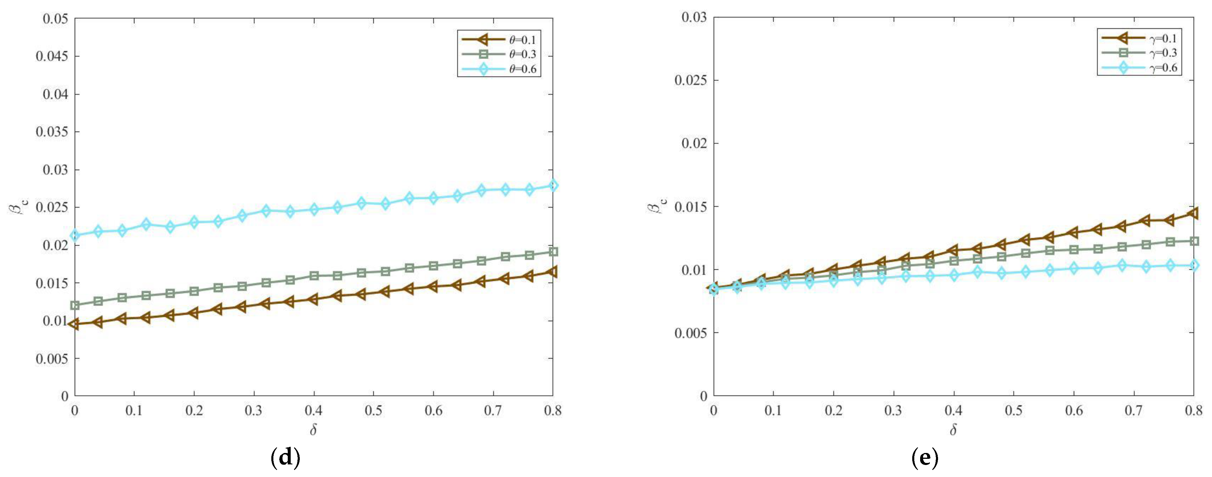
4. Numerical Simulation

We will verify the validity of MMCA through extensive MC simulations in this section, and test the effect of each parameter on risk diffusion scale and risk threshold in turn by MMCA. The initial structure of the two-layer network is set as follows: the initial number of nodes in the supply chain network is 16, and the other parameters are set as $\alpha =5$, $m=2$, $m_1=5$, $m_2=7$, $p=0.5$, $q=0.4$, an initial supply chain network with 1000 nodes is randomly generated according to Section 2.1. The initial social network has the same structure as the initial supply chain network but with 30 extra random hyperedges. In addition, the initial proportions of enterprises that believed uncertain information (B) and infected by risk (E) were set to 10% and 2%, respectively.

The proportion of enterp rise in the B-state and the R-state under steady state are the key indicators of risk diffusion in the supply chain network. For the MC simulation ${\rho }^B=\frac{N_B}{N}$, ${\rho }^R=\frac{N_R}{N}$, where $N_B$ and $N_R$ represent the number of B-state enterprise and R-state enterprise, respectively, $N$ represents the total number of nodes. For the MMCA, ${\rho }^B=\frac{1}{N}{\displaystyle \sum _{i=1}^N{P}_i^B}$, ${\rho }^R=\frac{1}{N}{\displaystyle \sum _{i=1}^N{P}_i^R}$, where $P_i^B$ and $P_i^R$ represent the probability of node $i$ in the B-state and R-state, respectively. ${\rho }^U$, ${\rho }^S$, ${\rho }^E$, and ${\rho }^I$ are represented similarly.

Firstly, Figure 5a depicts the change in the proportion of enterprise in U-state and B-state with the time $t$, and Figure 5b depicts the change in the proportion of enterprise in S-state, E-statue, I-state, and R-state with the time $t$. It can be seen that the results of MMCA are basically consistent with the results of MC, which shows that MMCA can be used to simulate the risk diffusion process under uncertain information. Besides, it is found that the proportion of B-state enterprise increased first, then decreased, and then rose to a steady state with the increase of the time $t$, where the proportion decreased because the I-state enterprise in the risk diffusion layer would automatically change to U-state in the virtual communication layer.

Secondly, Figure 6 compares the theoretical results of MMCA and the MC simulation results by describing the trend of the proportion ${\rho }^R$ of recovered nodes with the increase of infection rate $\beta$ under different attenuation factors $\gamma$. The basic agreement between the line and the dot reconfirms the effectiveness of MMCA. By calculation, the errors are 4.01%, 2.80%, and 2.80%, respectively when the attenuation factors are 0.2, 0.5, and 0.8. Therefore, we will use MMCA to test the effects of various parameters on risk diffusion scale and risk thresholds next.

Then, Figure 7 depicts the evolution trend of the recovery node proportion ${\rho }^R$ with increasing risk infected rate $\beta$ under different parameters $p$, $q$, $r$, $\theta$, and $\gamma$. It can be seen from Figure 7a,b and e that ${\rho }^R$ increases with the rise of parameters $p$, $q$ and the attenuation factor $\gamma$. Because $p$, $q$ represents the probability of adding new cooperation, much cooperation will accelerate the diffusion of risk, while the larger the attenuation factor, enterprises that do not trust uncertain information are more likely to be infected by risk. Additionally, In Figure 7c and d, ${\rho }^R$ decreases as the parameters $r$ and $\theta$ increase. Because $r$ represents the probability of adding nodes and removing old nodes, deleting outdated enterprises with great influence and introducing emerging enterprises with no risk is very effective in suppressing risk. The official media publishes market-related information many times, it is also helpful for enterprises to make correct judgments thereby reduce risk.

Furthermore, we explored the complete phase diagram $\delta -\beta$ to further analyze the effects of each parameter on risk diffusion. Figure 8, Figure 9 and Figure 10 reveals the impact of the dynamic evolution of the network on risk diffusion, the larger $p$ and $q$ will lead to larger ${\rho }^R$, while $r$ has the opposite effect on ${\rho }^R$. Figure 11 and Figure 12 denote the effect of uncertain information, the larger $\theta$ will lead to smaller ${\rho }^R$, while the effect of $\gamma$ is opposite. This is consistent with the above conclusion, i.e., reducing cooperation and the influence of uncertain information during the risk period, enhancing the work efficiency of the official media and the replacement efficiency of outdated enterprises in the market can effectively restrain the risk diffusion in the system.

Finally, Figure 13 reveals the relationship of parameters $p$, $q$, $r$, $\theta$, and $\gamma$ to risk thresholds ${\beta }_c$ with the increase of wakefulness rate $\delta$. From Figure 13a–c, it can be seen that the risk threshold gradually decreases with the increase of parameters $p$ and $q$, and increases as the parameter $r$ increases. Moreover, Figure 13d,e denotes that the risk threshold increases as the parameter $\theta$ increases and decreases as the attenuation factor increases. Therefore, the cooperation between enterprises and the influence of uncertain information should be reduced when risk spreads, the new enterprises should be increased to improve vitality in the market, the outdated enterprises should be eliminated to reduce the waste of resources, while the official media should correct the uncertain information to reduce distractions.

5. Conclusions

Considering the continuous disruption of supply chains under the influence of COVID-19, and the impact of uncertain information on supply chain risk diffusion, this paper introduces an official media that connects all enterprises in the virtual communication layer, and constructs a multi-layer dynamic hypernetwork framework to study the risk diffusion under uncertain information. Firstly, the risk diffusion scale and risk threshold are theoretically analyzed by MMCA. Then, the numerical simulation is carried out by MATLAB, and the consistency of the MC simulation and MMCA results are obtained. Finally, the effect of dynamic hypernetwork parameters, attenuation factor, and official media on risk diffusion are tested successively by MMCA, some rational suggestions are given.

This paper expounds on the importance of resisting uncertain information and weeding out outdated enterprises in the periods of risk diffusion, and draws the following conclusions First, accurate news from official media can effectively suppress the proliferation of uncertain information, thereby reducing risk diffusion. Second, enhancing the judging ability of enterprises so that they make more correct judgments in the risk environment, can reduce the probability of enterprises’ infection risks. Third, the formation of new enterprises and the elimination of outdated ones can curb the diffusion of risks. Since the real network is dynamic and the process of risk diffusion must be accompanied by the propagation of uncertain information, the risk diffusion mechanism under the uncertain information based on the hypernetwork is closer to reality. However, many factors will affect the cooperation of enterprises and the actual dynamic network topology is more complex, there is still a certain gap between our model and reality. More efforts on collecting actual data to further verify the validity of the model, or considering the risk diffusion in other environments to further improve the dynamic evolution of the network are expected in future works.

References

1. Heckmann, I.; Comes, T.; Nickel, S. A Critical Review on Supply Chain Risk—Definition, Measure and Modeling. Omega (U. K.) 2015, 52, 119–132. [Google Scholar] [CrossRef] [Green Version]
2. Wang, J.; Zhou, H.; Jin, X. Risk Transmission in Complex Supply Chain Network with Multi-Drivers. Chaos Solitons Fractals 2021, 143, 110259. [Google Scholar] [CrossRef]
3. Ran, M.; Chen, J. An Information Dissemination Model Based on Positive and Negative Interference in Social Networks. Phys. A Stat. Mech. Its Appl. 2021, 572, 125915. [Google Scholar] [CrossRef]
4. Kang, H.; Sun, M.; Yu, Y.; Fu, X.; Bao, B. Spreading Dynamics of an SEIR Model with Delay on Scale-Free Networks. IEEE Trans. Netw. Sci. Eng. 2020, 7, 489–496. [Google Scholar] [CrossRef]
5. He, D.; Liu, X. Novel Competitive Information Propagation Macro Mathematical Model in Online Social Network. J. Comput. Sci. 2020, 41, 101089. [Google Scholar] [CrossRef]
6. Garg, H.; Nasir, A.; Jan, N.; Khan, S.U. Mathematical Analysis of COVID-19 Pandemic by Using the Concept of SIR Model. Soft Comput. 2021, 1, 1–15. [Google Scholar] [CrossRef]
7. Hu, P.; Geng, D.; Lin, T.; Ding, L. Coupled Propagation Dynamics on Multiplex Activity-Driven Networks. Phys. A Stat. Mech. Its Appl. 2021, 561, 125212. [Google Scholar] [CrossRef]
8. Liu, H.; Yang, N.; Yang, Z.; Lin, J.; Zhang, Y. The Impact of Firm Heterogeneity and Awareness in Modeling Risk Propagation on Multiplex Networks. Phys. A Stat. Mech. Its Appl. 2020, 539, 122919. [Google Scholar] [CrossRef] [Green Version]
9. Huo, L.; Guo, H.; Cheng, Y.; Xie, X. A New Model for Supply Chain Risk Propagation Considering Herd Mentality and Risk Preference under Warning Information on Multiplex Networks. Phys. A Stat. Mech. Its Appl. 2020, 545, 123506. [Google Scholar] [CrossRef]
10. Qian, Q.; Feng, H.; Gu, J. The Influence of Risk Attitude on Credit Risk Contagion—Perspective of Information Dissemination. Phys. A Stat. Mech. Its Appl. 2021, 582, 126226. [Google Scholar] [CrossRef]
11. Zhang, M.; Qin, S.; Zhu, X. Information Diffusion under Public Crisis in BA Scale-Free Network Based on SEIR Model—Taking COVID-19 as an Example. Phys. A Stat. Mech. Its Appl. 2021, 571, 125848. [Google Scholar] [CrossRef]
12. Yin, H.; Wang, Z.; Xu, Z. Transmission Mechanism and Influencing Factors of Green Behavior in Dynamic Multiplex Networks. IEEE Access 2021, 9, 104382–104394. [Google Scholar] [CrossRef]
13. Denning, P.J. Supernetworks. Am. Sci. 1984, 73, 225–227. [Google Scholar]
14. Estrada, E.; Rodríguez-Velázquez, J.A. Subgraph Centrality and Clustering in Complex Hyper-Networks. Phys. A Stat. Mech. Its Appl. 2006, 364, 581–594. [Google Scholar] [CrossRef] [Green Version]
15. Suo, Q.; Guo, J.L.; Sun, S.; Liu, H. Exploring the Evolutionary Mechanism of Complex Supply Chain Systems Using Evolving Hypergraphs. Phys. A Stat. Mech. Its Appl. 2018, 489, 141–148. [Google Scholar] [CrossRef]
16. Wang, Z.; Yin, H.; Jiang, X. Exploring the Dynamic Growth Mechanism of Social Networks Using Evolutionary Hypergraph. Phys. A Stat. Mech. Its Appl. 2020, 544, 122545. [Google Scholar] [CrossRef]
17. Jiang, X.; Wang, Z.; Liu, W. Information Dissemination in Dynamic Hypernetwork. Phys. A Stat. Mech. Its Appl. 2019, 532, 121578. [Google Scholar] [CrossRef]
18. Meixell, M.J.; Gargeya, V.B. Global Supply Chain Design: A Literature Review and Critique. Transp. Res. Part E Logist. Transp. Rev. 2005, 41, 531–550. [Google Scholar] [CrossRef] [Green Version]
19. Ritchie, B.; Brindley, C. Disintermediation, Disintegration and Risk in the SME Global Supply Chain. Manag. Decis. 2000, 38, 575–583. [Google Scholar] [CrossRef]
20. Qi, S.; Jinli, G. Both Random and Preferential Attachment-the Inner Motivation in the Evolution of Hypernetworks. Complex Syst. Complex. Sci. 2016, 13, 52–55. [Google Scholar]
21. Yin, H.; Wang, Z.; Gou, Y.; Xu, Z. Rumor Diffusion and Control Based on Double-Layer Dynamic Evolution Model. IEEE Access 2020, 8, 115273–115286. [Google Scholar] [CrossRef]
22. Tian, X.; Chai, G.; Xie, Q.; Fan, M.; Qin, S.; Fan, C.; Gong, Y.; Liu, J.; Li, G. Risk Identification of Heavy Metals in Agricultural Soils from a Typically High Cd Geological Background Area in Upper Reaches of the Yangtze River. Bull. Environ. Contam. Toxicol. 2022, 109, 713–718. [Google Scholar] [CrossRef] [PubMed]
23. Ma, W.; Zhang, P.; Zhao, X.; Xue, L. The Coupled Dynamics of Information Dissemination and SEIR-Based Epidemic Spreading in Multiplex Networks. Phys. A Stat. Mech. Its Appl. 2022, 588, 126558. [Google Scholar] [CrossRef] [PubMed]
24. Yin, Q.; Wang, Z.; Xia, C.; Bauch, C.T. Impact of Co-Evolution of Negative Vaccine-Related Information, Vaccination Behavior and Epidemic Spreading in Multilayer Networks. Commun. Nonlinear Sci. Numer. Simul. 2022, 109, 106312. [Google Scholar] [CrossRef]
25. Guo, H.; Wang, Z.; Sun, S.; Xia, C. Interplay between Epidemic Spread and Information Diffusion on Two-Layered Networks with Partial Mapping. Phys. Lett. Sect. A Gen. At. Solid State Phys. 2021, 398, 127282. [Google Scholar] [CrossRef]
26. Mei, X.; Gong, G. Predicting Airborne Particle Deposition by a Modified Markov Chain Model for Fast Estimation of Potential Contaminant Spread. Atmos. Environ. 2018, 185, 137–146. [Google Scholar] [CrossRef]
Figure 1. Schematic diagram of dynamic network evolution. (iiii) are parallel relationships, one of them will happen at the next time step t + 1 . (i) add a new hyperedge e 3 consisting of nodes 3, 4, and 5; (ii) randomly select a link e 2 containing node 2 to disconnect and then form a new hyperedge e 4 with nodes 3 and 4; (iii) Node 5 exits, and nodes 6 and 7 enter the system.
Mathematics 10 04344 g001
Figure 2. Node state transition process. State transition diagram of uncertain information propagation on social networks (a) and State transition diagram of risk diffusion on supply chain network (b).
Mathematics 10 04344 g002
Figure 3. Schematic diagram of the model evolution mechanism. The virtual information layer has two node states: Unbelieve (orange), Believe (navy). The risk diffusion layer has four node states: Susceptible (blue), Exposed (pink), Infected (fuchsia), and Recovered (green). At each time step t , the upper and lower network structures evolve via Figure 1, processes (iiii) correspond to the three processes in Figure 1, respectively, i.e., addition of hyperedges, rewiring of hyperedges, entry and exit of nodes; the node status is updated via Figure 2. Hyperedges e 1 * represent the information exchange between non-cooperative enterprises.
Mathematics 10 04344 g003
Figure 4. State transition probability tree.
Mathematics 10 04344 g004
Figure 5. (a) Enterprise proportion of U, B states as a function of the time step t ; (b) Enterprise proportion of S, E, I, and R states as a function of the time step t . The model parameters are set as follows: p = 0.3 , q = 0.25 , α = 5 , m = 2 , m 1 = 5 , m 2 = 7 , κ = 2 , β = 0.9 , η = 0.6 , μ = 0.5 , λ = 0.5 , δ = 0.3 , γ = 0.5 , θ = 0 .
Mathematics 10 04344 g005
Figure 6. Comparison of MC simulation and MMCA results. The parameters are as follows: p = 0.5 , q = 0.5 , α = 5 , m = 2 , m 1 = 5 , m 2 = 7 , κ = 2 , η = 0.8 , μ = 0.8 , λ = 0.8 , δ = 0.2 , θ = 0 . 3 .
Mathematics 10 04344 g006
Figure 7. Effects of parameters p , q , r , θ and γ on recovery enterprises proportion ρ R . Other parameters are as follows: α = 5 , m = 2 , m 1 = 5 , m 2 = 7 , κ = 2 , η = 0.8 , μ = 0.8 , λ = 0.8 , δ = 0.2 , γ = 0 , θ = 0 , p = 0.5 , q = 0.5 . (a) the evolution trend of the recovery node proportion ρ R with increasing risk infected rate β under different parameters p .(b) the evolution trend of the recovery node proportion ρ R with increasing risk infected rate β under different parameters q . (c) the evolution trend of the recovery node proportion ρ R with increasing risk infected rate β under different parameters r . (d) the evolution trend of the recovery node proportion ρ R with increasing risk infected rate β under different parameters θ . (e) the evolution trend of the recovery node proportion ρ R with increasing risk infected rate β under different parameters γ .
Mathematics 10 04344 g007
Figure 8. The full-phase diagram δ β for different values of p . The color represents the proportion ρ R of recovered enterprise under steady state, other parameters are set as α = 5 , m = 2 , m 1 = 5 , m 2 = 7 , κ = 2 , η = 0.8 , μ = 0.8 , λ = 0.8 , γ = 0 , θ = 0 .
Mathematics 10 04344 g008
Figure 9. The full-phase diagram δ β for different values of q . The color represents the proportion ρ R of recovered enterprise under steady state, other parameters are set as α = 5 , m = 2 , m 1 = 5 , m 2 = 7 , κ = 2 , η = 0.8 , μ = 0.8 , λ = 0.8 , γ = 0 , θ = 0 .
Mathematics 10 04344 g009
Figure 10. The full-phase diagram δ β for different values of r . The color represents the proportion ρ R of recovered enterprise under steady state, other parameters are set as α = 5 , m = 2 , m 1 = 5 , m 2 = 7 , κ = 2 , η = 0.8 , μ = 0.8 , λ = 0.8 , γ = 0 , θ = 0 .
Mathematics 10 04344 g010
Figure 11. The full-phase diagram δ β for different values of θ . The color represents the proportion ρ R of recovered enterprise under steady state, other parameters are set as α = 5 , m = 2 , m 1 = 5 , m 2 = 7 , κ = 2 , η = 0.8 , μ = 0.8 , λ = 0.8 , γ = 0 , p = 0.5 , q = 0.5 .
Mathematics 10 04344 g011
Figure 12. The full-phase diagram δ β for different values of γ . The color represents the proportion ρ R of recovered enterprise under steady state, other parameters are set as α = 5 , m = 2 , m 1 = 5 , m 2 = 7 , κ = 2 , η = 0.8 , μ = 0.8 , λ = 0.8 , θ = 0.3 , p = 0.5 , q = 0.5 .
Mathematics 10 04344 g012
Figure 13. Effects of parameters p , q , r , θ and γ on risk threshold β c . The parameters are as follows: η = 0.5 , μ = 0.6 , λ = 0.9 . (a) α = 12 , m = 3 , m 1 = 1 , m 2 = 2 , κ = 3 , γ = 0 , θ = 0 . (b) α = 12 , m = 5 , m 1 = 1 , m 2 = 2 , κ = 3 , γ = 0 , θ = 0 . (c) α = 12 , m = 3 , m 1 = 1 , m 2 = 2 , κ = 3 , γ = 0 , θ = 0 . (d) α = 5 , m = 1 , m 1 = 2 , m 2 = 3 , p = 0.8 , q = 0.2 , κ = 2 , γ = 0 . (e) α = 5 , m = 1 , m 1 = 2 , m 2 = 3 , p = 0.8 , q = 0.2 , κ = 2 , θ = 0 .
Mathematics 10 04344 g013aMathematics 10 04344 g013b