Article

Steady-State Solutions for MHD Motions of Burgers’ Fluids through Porous Media with Differential Expressions of Shear on Boundary and Applications

1
Section of Mathematics, Academy of Romanian Scientists, 050094 Bucharest, Romania
2
Department of Computer Science and Engineering, Air University Islamabad, Islamabad 44000, Pakistan
3
Department of Mathematics, COMSATS University Islamabad, Vehari Campus, Vehari 61100, Pakistan
4
Department of Theoretical Mechanics, Technical University of Iasi, 700050 Iasi, Romania
*
Author to whom correspondence should be addressed.
Mathematics 2022, 10(22), 4228; https://doi.org/10.3390/math10224228
Submission received: 9 October 2022 / Revised: 2 November 2022 / Accepted: 8 November 2022 / Published: 12 November 2022

Abstract

:
Steady-state solutions for two mixed initial-boundary value problems are provided. They describe isothermal MHD steady-state motions of incompressible Burgers’ fluids over an infinite flat plate embedded in a porous medium when differential expressions of shear stress are given on a part of the boundary. The fluid is electrically conductive under the influence of a uniform transverse magnetic field. For the validation of the results, the expressions of the obtained solutions are presented in different forms and their equivalence is graphically proved. All of the obtained results could easily be particularized to give exact solutions for the incompressible Oldroyd-B, Maxwell, second-grade, and Newtonian fluids that were performing similar motions. For illustration, the solutions corresponding to Newtonian fluids are provided. In addition, as an application, the velocity fields were used to determine the time required to reach the steady or permanent state for distinct values of magnetic and porous parameters. We found that this time declined with increasing values of the magnetic or porous parameters. Consequently, the steady state for such motions of Burgers’ fluids was earlier reached in the presence of a magnetic field or porous medium.

1. Introduction

The isothermal motions of incompressible Newtonian or non-Newtonian fluids over an infinite plate have been extensively studied in the past. They are some of the most important motion problems near moving bodies and have multiple industrial applications including the processing of polymers, food products, pharmaceuticals, clay suspensions, and many others. Generally, in practice, an infinite plate cannot be used. However, its dimensions can be large enough so that the solutions corresponding to motions over such a plate can be sufficiently approximated by solutions for motions over an infinite plate. In the existing literature, there are many studies on the motion problems of fluids over an infinite plate or between two infinite parallel plates. The most recent results regarding oscillatory motions of incompressible Burgers’ fluids over an infinite plate seem to be those of Akram et al. [1]. The MHD motions of these fluids also have different applications in hydrology, horticulture, and engineering structures. The exact solutions for the MHD second Stokes flow of the same fluids can be obtained from the work of Khan et al. [2]. In addition, the study of different motions through porous media has a distinguished importance in different fields, including those in the natural sciences and technology. Hydrodynamic studies of the Maxwell fluid flow through a porous medium were recently provided by Ullah et al. [3] and Fetecau et al. [4]. Exact solutions for MHD unsteady motions of incompressible non-Newtonian fluids over an infinite flat plate embedded in a porous medium were previously established; for instance, by Hayat et al. [5] and Ali et al. [6] for second-grade fluids, Khan et al. [7] for Oldroyd-B fluids, and Algahtani and Khan [8] and Hussain et al. [9] for Burgers’ fluids. General solutions for isothermal MHD motions of incompressible Newtonian fluids over an infinite plate embedded in a porous medium were obtained by Fetecau et al. [10]. The combined effects of free convection MHD flow past a vertical plate embedded in a porous medium were recently investigated by Vijayalakshmi et al. [11].
Many exact solutions for MHD unsteady motions of the incompressible non-Newtonian fluids over an infinite plate embedded in a porous medium were determined previously by different authors. However, Khan et al. [2] seemed to be the first authors who established exact solutions for such motions of incompressible Burgers’ fluids. The one-dimensional form of the constitutive equation of incompressible Burgers’ fluids was proposed by Burgers [12]; his model is often used to describe the behavior of different viscoelastic materials such as polymeric liquids, cheese, soil, and asphalt [13,14]. A good agreement between the prediction of this model and the behavior of asphalt and sand-asphalt was found by Lee and Markwick [15]. The extension of the one-dimensional Burgers’ model to a frame-indifferent three-dimensional form was provided by Krishnan and Rajagopal [16], while the first exact steady solutions for motions of such fluids seem to be those of Ravindran et al. [17] for a fluid flow in an orthogonal rheometer. Other interesting solutions for oscillatory motions of incompressible Burgers’ fluids were established by Hayat et al. [18], Khan et al. [19,20], and recently Safdar et al. [21]. Exact steady-state solutions for isothermal motions of same fluids when a differential expression of shear stress was given on a part of the boundary were recently obtained by Fetecau et al. [22]. In order to study similar flows of the same fluids in bounded domains, which are useful in industrial applications, readers can use the recent works by Çolak et al. [23] and Abderrahmane et al. [24].
Earlier, Renardy [25,26] showed that boundary conditions containing differential expressions of stresses must be imposed in order to formulate well-posed boundary value problems for motions of rate-type fluids. The main purpose of this work was to provide the first exact steady-state solutions for motions of incompressible Burgers’ fluids, which are rate-type fluids, when differential expressions of the shear stress were given on a part of the boundary and the magnetic and porous effects were taken into consideration. These solutions, which are presented in simple forms, could easily be particularized to give exact solutions for incompressible Oldroyd-B, Maxwell, second-grade and Newtonian fluids that were performing similar motions. For illustration, the adequate solutions for the Newtonian fluids are brought to light. In addition, for the validation of the results, all of the solutions are presented in different forms and their equivalence is graphically proved. Finally, as an application, the required time to reach the steady or permanent state was graphically determined for distinct values of the magnetic and porous parameters.

2. Statement of the Problem

Consider an incompressible, electrically conducting Burgers’ fluid (IECBF) at rest over an infinite horizontal flat plate embedded in a porous medium. Its constitutive equations, as presented by Ravindran et al. [15], are given by the relations:
T = p I + S , S + α D S D t + β D 2 S D t 2 = μ A + γ D A D t ,
where T is the Cauchy stress tensor; S is the extra-stress tensor; I is the unit tensor; A = L + L T is the first Rivlin–Ericksen tensor (L being the gradient of the velocity vector υ ); p is the hydrostatic pressure; μ is the fluid viscosity; α ,     β , and γ   ( α ) are material constants; and D/Dt denotes the well-known upper-convected derivative. Since the incompressible fluids undergo isochoric motions only, the following continuity equation must be satisfied:
div υ = 0 or equivalent tr A = 0 .
We also most consider the fact that the fluids characterized by the constitutive Equation (1) contain the incompressible Oldroyd-B, Maxwell, and Newtonian fluids as special cases if β = 0 ,   β = γ = 0 , or α = β = γ = 0 , respectively. For the motions to be considered here, the governing equations corresponding to the incompressible second-grade fluids can also be obtained as particular cases of the present equations.
In the following, and based on Khan et al. [2], we shall consider isothermal MHD unsteady motions of an IECBF over an infinite flat plate embedded in a porous medium for which
υ = υ ( y , t ) = u ( y , t ) e x , S = S ( y , t ) ,
where e x is the unit vector along the x-direction of a convenient Cartesian coordinate system of x, y, and z with the y-axis perpendicular to the plate. For such motions, the continuity equation is identically satisfied. Substituting υ ( y , t ) and S ( y , t ) from Equation (3) in the second equality from the relations in (1) and bearing in mind the fact that the fluid has been at rest up to the initial moment t = 0 , one can prove that the components   S y y ,   S y z ,   S z z   and S z x of S are zero. On the other hand, the non-trivial shear stress τ ( y , t ) = S x y ( y , t ) must satisfy the next partial differential equation [18].
1 + α t + β 2 t 2 τ ( y , t ) = μ 1 + γ t u ( y , t ) y ;       y > 0 ,       t > 0 .
The balance of linear momentum in the presence of conservative body forces and of a transverse magnetic field of the magnitude B but in the absence of a pressure gradient in the flow direction reduces to the following partial differential equation [2]:
ρ u ( y , t ) t = τ ( y , t ) y σ B 2 u ( y , t ) + R ( y , t ) ;       y > 0 ,       t > 0 ,
where ρ is the constant density of the fluid, σ is its electrical conductivity, and the Darcy’s resistance R ( y , t ) satisfies the relation [2].
1 + α t + β 2 t 2 R ( y , t ) = μ φ k 1 + γ t u ( y , t ) ;       y > 0 ,       t > 0 .
In the above relation, φ and k are the porosity and the permeability, respectively, of the porous medium.
The appropriate initial conditions of:
u ( y , 0 ) = u ( y , t ) t t = 0 = 2 u ( y , t ) t 2 t = 0 = 0 ; τ ( y , 0 ) = τ ( y , t ) t t = 0 = 0 ;       y 0 ,    
have been already used to show that some of the components of the extra-stress S are zero. The boundary conditions to be here used are given by the following relations:
1 + α t + β 2 t 2 τ ( 0 , t ) = μ 1 + γ t u ( y , t ) y y = 0 = S cos ( ω t ) ,       lim y u ( y , t ) = 0 ;       t > 0 ,
or
1 + α t + β 2 t 2 τ ( 0 , t ) = μ 1 + γ t u ( y , t ) y y = 0 = S sin ( ω t ) ,       lim y u ( y , t ) = 0 ;       t > 0 .
In the above relations, S is a constant shear stress and ω is the frequency of the oscillations.
The second condition from the relations (8) and (9) assures us that the fluid is quiescently far away from the plate. We also assume that there is no shear in the free stream; i.e.,:
lim y τ ( y , t ) = 0 .
For convenience, we also assume that the fluid is finitely conducting so that the Joule heating due to the presence of external magnetic field is negligible. In addition, the magnetic Reynolds number is small enough so that the induced magnetic field can be neglected and the electromagnetic energy does not penetrate the boundary for computing the Umov–Poynting vector [27]. Moreover, there is no surplus electric charge distribution present in the fluid and the Hall effects can be ignored due to moderate values of the Hartman number.
In order to provide exact solutions that are independent of the flow geometry, let us introduce the next dimensionless functions, variables and parameters:
u = u ρ S ,         τ = τ S ,       R = ν ρ S S R ,       y = y S μ ν ,       t = S μ t , α = S μ α ,     β = S 2 μ 2 β ,       γ = S μ γ ,       ω = μ S ω   .
Using the non-dimensional entities from the relations in (11) in the equalities (4)–(6) and abandoning the star notation for writing simplicity, one obtains the non-dimensional forms of these equations:
1 + α t + β 2 t 2 τ ( y , t ) = 1 + γ t u ( y , t ) y ;       y > 0 ,       t > 0 ,
u ( y , t ) t = τ ( y , t ) y M u ( y , t ) + R ( y , t ) ;       y > 0 ,       t > 0 ,
1 + α t + β 2 t 2 R ( y , t ) = K 1 + γ t u ( y , t ) ;       y > 0 ,       t > 0 ,
where the constants M and K are the magnetic and porous parameters, respectively, which are defined by the following relations:
M = σ B 2 ρ   μ S = ν S σ B 2 , K = μ ν φ k S = μ φ k   ν S .
When eliminating τ ( y , t ) between Equations (12) and (13) and bearing in mind Equation (14), one obtains for the dimensionless velocity field u ( y , t ) the following partial differential equation:
1 + α t + β 2 t 2 u ( y , t ) t = 1 + γ t 2 u ( y , t ) y 2 M 1 + α t + β 2 t 2 u ( y , t ) K 1 + γ t u ( y , t ) ;       y > 0 ,       t > 0 .
The corresponding boundary conditions are given by the next equalities:
1 + α t + β 2 t 2 τ ( 0 , t ) = 1 + γ t u ( y , t ) y y = 0 = cos ( ω t ) ,         lim y u ( y , t ) = 0 ;         t > 0 ,
or
1 + α t + β 2 t 2 τ ( 0 , t ) = 1 + γ t u ( y , t ) y y = 0 = sin ( ω t ) ,         lim y u ( y , t ) = 0 ;         t > 0 .
The adequate initial conditions have the same forms as in Equation (7) but they will not be used in the following because only steady-state (permanent or long-term) solutions will be provided. The non-dimensional shear stress τ ( y , t ) also must satisfy the following condition:
lim y τ ( y , t ) = 0 .
The form of the boundary conditions in (17) and (18), as well as the fact that the fluid was at rest at the moment t = 0 , suggests that the two motions become steady in time. For such motions, a very important problem for experimental researchers is to know the time needed to reach the steady or permanent state. This is the time after which the fluid moves according to the steady-state solutions. In the following, in order to avoid a possible confusion, we denote by u c ( y , t ) , τ c ( y , t ) , R c ( y , t ) and u s ( y , t ) , τ s ( y , t ) , R s ( y , t ) the starting solutions corresponding to the two fluid motions whose boundary conditions are given by the relations in (17) and (18), respectively. These solutions, which characterize the fluid motion some time after its initiation, can be written as sum of their respective steady-state and transient components; i.e.,:
u c ( y , t ) = u c p ( y , t ) + u c t ( y , t ) ,       τ c ( y , t ) = τ c p ( y , t ) + τ c t ( y , t ) ,       R c ( y , t ) = R c p ( y , t ) + R c t ( y , t ) ,
and
u s ( y , t ) = u s p ( y , t ) + u s t ( y , t ) ,       τ s ( y , t ) = τ s p ( y , t ) + τ s t ( y , t ) ,       R s ( y , t ) = R s p ( y , t ) + R s t ( y , t ) .
After this time, when the transients disappear or can be negligible, the fluid behavior is described by the steady-state or permanent solutions u c p ( y , t ) , τ c p ( y , t ) , R c p ( y , t ) or u s p ( y , t ) , τ s p ( y , t ) , R s p ( y , t ) . In order to determine this time for a given motion, at least the steady-state or transient solutions have to be known. Since, for the transient solutions of the motions, we do not know a modality to verify their correctness, in the following we shall provide closed-form expressions for the steady-state solutions of the two above-mentioned motion problems. These steady-state solutions, which are independent of the initial conditions, satisfy the boundary conditions and governing equations.

3. Dimensionless Steady-State Solutions

In this section, we provide closed-form expressions for the dimensionless steady-state velocity and shear stress fields u c p ( y , t ) , u s p ( y , t ) and τ c p ( y , t ) , τ s p ( y , t ) , respectively, and the corresponding Darcy’s resistances R c p ( y , t ) ,     R s p ( y , t ) . For a check of the obtained results, these expressions are presented in different forms and their equivalence is graphically proved.

3.1. Calculation of the Steady-State Velocities u c p ( y , t ) and u s p ( y , t )

To determine the dimensionless velocity fields u c p ( y , t ) and u s p ( y , t ) that satisfy the governing Equation (16) and the respective boundary conditions (17) and (18), we follow two different methods. Firstly, while bearing in mind the linearity of the governing Equation (16) and the form of the boundary conditions (17) and (18), we define the steady-state complex velocity:
u p ( y , t ) = u c p ( y , t ) + i u s p ( y , t ) ;       y > 0 ,       t R ,
where i is the imaginary unit and is searching for a solution of the form:
u p ( y , t ) = U ( y ) e i ω t ;       y > 0 ,       t R ,
where U ( ) is a complex function. Of course, the dimensionless complex velocity u p ( y , t ) must satisfy the governing Equation (16) and the boundary conditions.
1 + γ t u p ( y , t ) y y = 0 = e i ω t , lim y u p ( y , t ) = 0 ; t R .
Direct computations show that u p ( y , t ) can be presented in the following form:
u p ( y , t ) = 1 ( 1 + i ω γ ) δ e δ y + i ω t ;       y > 0 ,       t R ,
while the dimensionless steady-state velocity fields u c p ( y , t ) and u s p ( y , t ) are given by the following relations:
u c p ( y , t ) = Re 1 ( 1 + i ω γ ) δ e δ y + i ω t , u s p ( y , t ) = Im 1 ( 1 + i ω γ ) δ e δ y + i ω t ,
where Re and Im denote the real and imaginary parts, respectively, of that which follows, and:
δ = ( 1 β ω 2 + i ω α ) ( M + i ω ) + K ( 1 + i ω γ ) 1 + i ω γ .
Secondly, in order to determine the equivalent forms for the dimensionless steady-state solutions given by Equation (26), we use the dimensionless steady-state solutions:
u S c p ( y , t ) = e m y cos ( ω t n y ) ,       u S s p ( y , t ) = e m y sin ( ω t n y ) ,
of the second problem of Stokes for incompressible Burgers’ fluids. It is the fluid motion over an infinite flat plate that oscillates in its plane with the dimensionless velocity cos ( ω t ) or sin ( ω t ) . In these solutions, which were determined by direct computations, the constants m and n are given by the following relations:
m = ω 2 a ω + ( a ω ) 2 + b 2 1 + ( γ ω ) 2 ,         n = ω 2 a ω + ( a ω ) 2 + b 2 1 + ( γ ω ) 2 ,
which satisfy the algebraic system of equations:
m 2 n 2 = a ω 2 1 + ( γ ω ) 2 ,         m n = b ω 2 [ 1 + ( γ ω ) 2 ] ,
where a and b are defined by following equalities:
a = γ ( 1 β ω 2 ) α ,         b = 1 β ω 2 + α γ ω 2 .
More precisely, we are looking for the present dimensionless steady-state velocity fields u c p ( y , t ) and u s p ( y , t ) under the following forms:
u c p ( y , t ) = p 1 u S c p ( y , t ) + q 1 u S s p ( y , t ) , u s p ( y , t ) = p 2 u S c p ( y , t ) + q 2 u S s p ( y , t ) .
They must satisfy the respective boundary conditions in (17) and (18). Lengthy but straightforward computations show that u c p ( y , t ) and u s p ( y , t ) can be presented in the following simple forms:
u c p ( y , t ) = p 2 + q 2   e m ˜ y cos ( ω t n ˜ y + φ ) , u s p ( y , t ) = p 2 + q 2   e m ˜ y sin ( ω t n ˜ y + φ ) .
In the last two relations, the angle φ = arctg ( q / p ) while the constants m ˜ , n ˜ , p, and q have the following expressions:
m ˜ = ω 2 c ω + ( c ω ) 2 + d 2 1 + ( γ ω ) 2 ,         n ˜ = ω 2 c ω + ( c ω ) 2 + d 2 1 + ( γ ω ) 2 ,
p = n ˜ ω γ m ˜ ( m ˜ ω γ + n ˜ ) 2 + ( n ˜ ω γ m ˜ ) 2 ,         q = m ˜ ω γ + n ˜ ( m ˜ ω γ + n ˜ ) 2 + ( n ˜ ω γ m ˜ ) 2 ,
in which c and d are given by the following relations:
c = γ ( 1 β ω 2 ) α + ( 1 β ω 2 + α γ ω 2 ) M + [ 1 + ( γ ω ) 2 ] K ω 2 , d = 1 β ω 2 + α γ ω 2 + [ α γ ( 1 β ω 2 ) ] M .
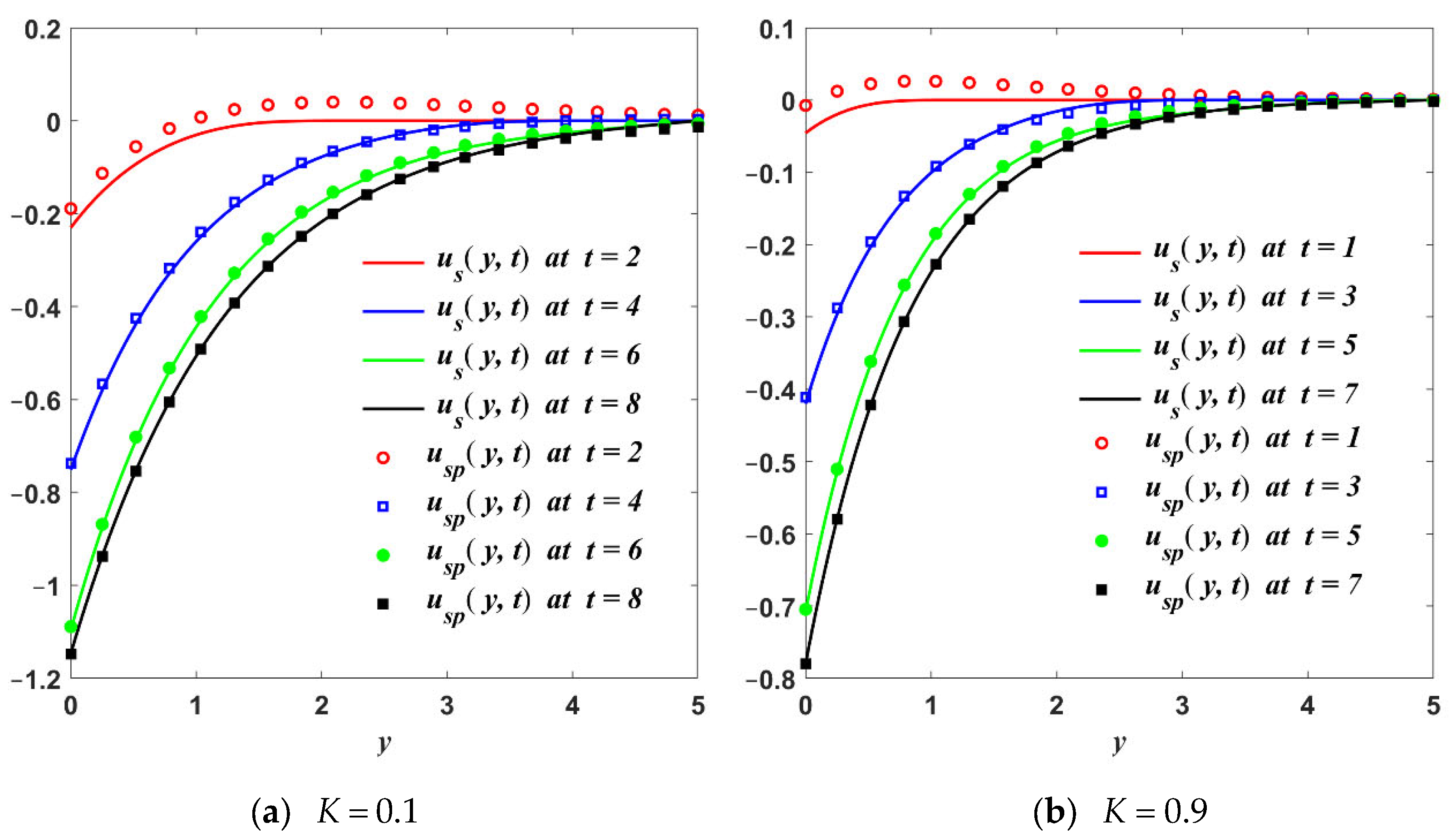
The equivalence of the dimensionless steady-state solutions given by the equalities in (26) and (33) is graphically proved in Figure 1a,b.
The dimensionless steady-state velocity fields u c p ( y , t ) and u s p ( y , t ) corresponding to isothermal motions of the same fluids in the absence of magnetic or porous effects can immediately be obtained by taking M = 0 , respectively K = 0 in Equations (26) and (33), respectively. In the absence of both effects, when M = K = 0 , the present solutions reduce to those obtained by Fetecau et al. [22] (Equations (19) and (20)). Moreover, the dimensionless steady-state solutions corresponding to incompressible Oldroyd-B, Maxwell, and Newtonian fluids that are performing similar motions are immediately obtained by taking β = 0 ,     β = γ = 0 or α = β = γ = 0 , respectively, in the previous relations. The dimensionless steady-state velocity fields corresponding to motions of the incompressible Newtonian fluids over an infinite flat plate that apply an oscillatory shear stress S cos ( ω t ) or S sin ( ω t ) to the fluid, for instance, have the following simple forms:
u N c p ( y , t ) = Re 1 K e f f + i ω e y K e f f + i ω + i ω t   , u N s p ( y , t ) = Im 1 K e f f + i ω e y K e f f + i ω + i ω t   ,
or the equivalent
u N c p ( y , t ) = 1 K e f f 2 + ω 2 4   e f y cos ( ω t g y + ψ ) , u N s p ( y , t ) = 1 K e f f 2 + ω 2 4   e f y sin ( ω t g y + ψ ) ,
where
f = K e f f + K e f f 2 + ω 2 2 ,       g = K e f f + K e f f 2 + ω 2 2 ,       ψ = arctg K e f f K e f f 2 + ω 2 ω
and K e f f = M + K is the effective permeability [10]. The equivalence of the solutions in (37) and (38) is graphically proved in Figure 2a,b.

3.2. Exact Expressions for τ c p ( y , t ) , τ s p ( y , t ) and R c p ( y , t ) ,     R s p ( y , t )

In order to determine the dimensionless steady-state shear stresses τ c p ( y , t ) , τ s p ( y , t ) and the Darcy’s resistances R c p ( y , t ) ,     R s p ( y , t ) corresponding to the two unsteady motions of the IECBF when magnetic and porous effects are taken into account, we firstly use the complex shear stress and Darcy’s resistance:
τ p ( y , t ) = τ c p ( y , t ) + i τ s p ( y , t ) , R p ( y , t ) = R c p ( y , t ) + i R s p ( y , t )
and follow the same method as for the steady-state velocities. The obtained results when using for u c p ( y , t ) and u s p ( y , t ) the expressions from the equalities in (26) are given by the following respective relations:
τ c p ( y , t ) = Re 1 1 β ω 2 + i ω α e δ y + i ω t , τ s p ( y , t ) = Im 1 1 β ω 2 + i ω α e δ y + i ω t ,
and
R c p ( y , t ) = K Re 1 ( 1 β ω 2 + i ω α ) δ e δ y + i ω t , R s p ( y , t ) = K Im 1 ( 1 β ω 2 + i ω α ) δ e δ y + i ω t .
Direct computations clearly show that the dimensionless steady-state velocity, shear stress, and Darcy’s resistance fields u c p ( y , t ) ,   τ c p ( y , t ) ,   R c p ( y , t ) and u s p ( y , t ) ,   τ s p ( y , t ) ,   R s p ( y , t ) given by the relations in (26), (41), and (42) satisfy the governing Equations (12)–(14) and the respective boundary conditions in (17) and (18).
Equivalent expressions for τ c p ( y , t ) ,   τ s p ( y , t ) and R c p ( y , t ) ,   R s p ( y , t ) , namely:
τ c p ( y , t ) = p 1 2 + q 1 2   e m ˜ y cos ( ω t n ˜ y + φ χ ) , τ s p ( y , t ) = p 1 2 + q 1 2   e m ˜ y sin ( ω t n ˜ y + φ χ ) ,
and
R c p ( y , t ) = p 2 2 + q 2 2   e m ˜ y cos ( ω t n ˜ y + φ θ ) , R s p ( y , t ) = p 2 2 + q 2 2   e m ˜ y sin ( ω t n ˜ y + φ θ ) ,
were obtained by using the corresponding velocity fields u c p ( y , t ) and u s p ( y , t ) from the equalities in (33). In these relations:
p 1 = ( 1 β ω 2 ) ( m ˜ n ˜ ω γ ) + α ω ( n ˜ + m ˜ ω γ ) ( 1 β ω 2 ) 2 + ( α ω ) 2 p 2 + q 2 , q 1 = α ω ( m ˜ n ˜ ω γ ) ( 1 β ω 2 ) ( n ˜ + m ˜ ω γ ) ( 1 β ω 2 ) 2 + ( α ω ) 2 p 2 + q 2 ,
p 2 = K 1 β ω 2 + α γ ω 2 ( 1 β ω 2 ) 2 + ( α ω ) 2 p 2 + q 2 ,     q 2 = ω K α γ ( 1 β ω 2 ) ( 1 β ω 2 ) 2 + ( α ω ) 2 p 2 + q 2 ,
where χ = arctg ( q 1 / p 1 ) and θ = arctg ( q 2 / p 2 ) . The equivalence of the dimensionless shear stresses τ c p ( y , t ) ,   τ s p ( y , t ) and of the Darcy’s resistances R c p ( y , t ) ,     R s p ( y , t ) given by Equation (41) and (42), respectively, to those from the relations in (43) and (44) is proved in Figure 3 and Figure 4.
The dimensionless steady-state shear stresses and Darcy’s resistances corresponding to the velocity fields u N c p ( y , t ) and u N s p ( y , t ) of incompressible Newtonian fluids given by the relations in (37) and (38) have the following simple forms:
τ N c p ( y , t ) = Re   e y K e f f + i ω + i ω t , τ N s p ( y , t ) = Im e y K e f f + i ω + i ω t ,
R N c p ( y , t ) = K Re 1 K e f f + i ω e y K e f f + i ω + i ω t , R N s p ( y , t ) = K Im 1 K e f f + i ω e y K e f f + i ω + i ω t ,
or the equivalent:
τ N c p ( y , t ) =   e f y cos ( ω t g y ) ,       τ N s p ( y , t ) =   e f y sin ( ω t g y ) ,
R N c p ( y , t ) = K K e f f 2 + ω 2 4   e f y cos ( ω t g y + ψ ) , R N s p ( y , t ) = K K e f f 2 + ω 2 4   e f y sin ( ω t g y + ψ ) .

4. Some Numerical Results and Applications

Closed-form expressions for the dimensionless steady-state solutions u c p ( y , t ) , τ c p ( y , t ) , R c p ( y , t ) and u s p ( y , t ) , τ s p ( y , t ) , R s p ( y , t ) corresponding to two isothermal MHD motions of an IECBF over an infinite flat plate embedded in a porous medium were presented in simple forms in the previous section. They are the first exact solutions for MHD motions of an IECBF with differential expressions of shear stress on the boundary. For validation, all solutions are presented in double forms and their equivalence was graphically proved. These solutions can easily be particularized to give corresponding solutions for incompressible Oldroyd-B, Maxwell, and Newtonian fluids that are performing similar motions.
As an application, some of the obtained results were used to determine the required time to reach the steady or permanent state. From a mathematical point of view, this was the time after which the diagrams of the starting velocities u c ( y , t ) and u s ( y , t ) (numerical solutions) were almost identical to those of their steady-state components u c p ( y , t ) and u s p ( y , t ) , respectively. The convergence of the two starting velocities to their steady-state components was proved in Figure 5, Figure 6, Figure 7 and Figure 8 for increasing values of the time t at distinct values of M and K and fixed values of the other parameters. Based on these figures, it was clear that the required time to reach the steady state diminished with increasing values of the magnetic or porous parameters (M and K, respectively). Consequently, the steady state for isothermal motions of the IECBF was earlier reached in the presence of a magnetic field or porous medium. In addition, as expected, in all cases the fluid velocity tended to zero with increasing values of the spatial variable y.
For comparison, as well as to bring to light some characteristic features of the two motions, the spatial distributions of the dimensionless starting velocity fields u c ( y , t ) and u s ( y , t ) (numerical solutions) are presented together in Figure 9a,b, respectively, for the same values of the physical parameters. The oscillatory behavior of the two motions, as well as the phase difference between them, can be easily observed. In addition, the initial and boundary conditions were clearly satisfied. Blue and yellow colors were used in the current figure to designate the minimum and maximum values of the two solutions, respectively. The intermediate values between the maximum and minimum are denoted by the gradient of the colors between yellow and blue.
The three-dimensional distributions of the same non-dimensional starting velocities u c ( y , t ) and u s ( y , t ) are also visualized by means of the two-dimensional contour graphs (see, for example, the paper of Fullard and Wake [28]) in Figure 10a,b, respectively, for α = 0.8 ,     β = 0.7 ,     γ = 0.6 ,     ω = π / 12 ,     M = 0.6 , and K = 0.4 .

5. Conclusions

Some unsteady motions of incompressible fluids become steady or permanent in time if the fluid is at rest at the initial moment. Of course, this also depends on the boundary conditions. For such motions, in practice, a very important problem is to know the time required to reach the steady or permanent state. This is the time after which the fluid moves according to the steady-state solutions. In order to determine this time for a given motion, it is sufficient to know the corresponding steady-state solutions. This is the reason why we established closed-form expressions for the dimensionless steady-state solutions corresponding to two isothermal MHD unidirectional motions of an IECBF over an infinite flat plate embedded in a porous medium. The boundary conditions that were used, contrary to what is usually found in the existing literature, contained differential expressions of the non-trivial shear stress on a part of the boundary. For a check of results that were obtained here, all solutions have been presented in different forms and their equivalence was graphically proved.
It is worth pointing out the fact that all of the obtained solutions could easily be particularized to give dimensionless steady-state solutions for the incompressible Oldroyd-B, Maxwell, second-grade and Newtonian fluids that were performing similar motions. By taking α = β = γ = 0 , for instance, dimensionless steady-state solutions corresponding to motions of an incompressible Newtonian fluid induced by the flat plate that applied a shear stress S cos ( ω t ) or S sin ( ω t ) to the fluid were brought to light. In addition, the solutions for motions of Burgers’ fluids were used to determine the required time to reach the steady state. This time, which in practice is very important for experimental researchers, was graphically determined by showing the convergence of the starting solutions to the corresponding steady-state solutions. The oscillatory behavior of the two motions, as well as the phase difference between them, was graphically underlined. The main outcomes that were here obtained are:
-
The first exact solutions for MHD motions of Burgers’ fluids through a porous medium were determined when differential expressions of shear stress were given on the boundary.
-
The solutions corresponding to Oldroyd-B, Maxwell, and Newtonian fluids that were performing similar motions were immediately obtained as limiting cases of the present results.
-
The convergence of the dimensionless starting velocities u c ( y , t ) and u s ( y , t ) to their respective steady-state components u c p ( y , t ) and u s p ( y , t ) was graphically proved. In addition, all of the obtained solutions were presented in different forms and their equivalence was proved.
-
The steady state for isothermal motions of incompressible Burgers fluids’ was earlier reached in the presence of a magnetic field or porous medium.

Author Contributions

Conceptualization, C.F., D.V. and A.R.; Methodology, C.F., D.V. and A.R.; Software, T.M.Q. and A.R.; Validation, C.F., D.V., A.R. and T.M.Q.; Writing—review and editing, C.F., D.V., A.R. and T.M.Q. All authors have read and agreed to the published version of the manuscript.

Funding

This research received no external funding.

Acknowledgments

The authors would like to express their gratitude to the Editor and reviewers for their careful assessments, kind appreciations, and fruitful suggestions regarding the first version of the manuscript.

Conflicts of Interest

The authors declare no conflict of interest.

Nomenclature

TCauchy stress tensorSExtra-stress tensor
AFirst Rivlin–Ericksen tensorLVelocity gradient
uFluid velocitySConstant shear stress
pHydrostatic pressurex, y, ZCartesian coordinates
R ( y , t ) Darcy’s resistancekPermeability of porous medium
MMagnetic parameterKPorous parameter
BMagnitude of magnetic field S y y ,   S y z ,   S z z ,   S z x   Components of S
Greek Symbols
τ Non-trivial shear stress ρ Fluid density
μ Dynamic viscosity ν Kinematic viscosity
υ Velocity vector σ Electrical conductivity
α ,   β ,   γ Material constants φ Porosity
ω Frequency of oscillations

References

  1. Akram, S.; Anjum, A.; Khan, M.; Hussain, A. On Stokes’ second problem for Burgers’ fluid over a plane wall. J. Appl. Comput. Mech. 2021, 7, 1514–1526. [Google Scholar]
  2. Khan, M.; Malik, R.; Anjum, A. Exact solutions of MHD second Stokes flow of generalized Burgers fluid. Appl. Math. Mech.–Engl. 2015, 36, 211–224. [Google Scholar] [CrossRef]
  3. Ullah, H.; Lu, D.; Siddiqui, A.M.; Haroon, T.; Maqbool, K. Hydrodynamical study of creeping Maxwell fluid flow through a porous slit with uniform reabsorption and wall slip. Mathematics 2020, 8, 1852. [Google Scholar] [CrossRef]
  4. Fetecau, C.; Ellahi, R.; Sait, S.M. Mathematical analysis of Maxwell fluid flow through a porous plate channel induced by a constantly accelerating or oscillating wall. Mathematics 2021, 9, 90. [Google Scholar] [CrossRef]
  5. Hayat, T.; Khan, I.; Ellahi, R.; Fetecau, C. Some MHD flows of a second grade fluid through the porous medium. J. Porous Media 2008, 11, 389–400. [Google Scholar] [CrossRef]
  6. Ali, F.; Norzieha, M.; Sharidan, S.; Khan, I.; Hayat, T. New exact solutions of Stokes’ second problem for an MHD second grade fluid in a porous space. Int. J. Non-Linear Mech. 2012, 47, 521–525. [Google Scholar] [CrossRef]
  7. Khan, M.; Khan, S.B.; Hayat, T. Exact solution for the magnetohydrodynamic flows of an Oldroyd-B fluid through porous medium. J. Porous Media 2007, 10, 391–399. [Google Scholar] [CrossRef]
  8. Alqahtami, A.M.; Khan, I. Time-dependent MHD flow of non-Newtonian generalized Burgers’ fluid over a suddenly moved plate with generalized Darcy’ law. Front. Phys. 2020, 7, 214. [Google Scholar] [CrossRef]
  9. Hussain, M.; Qayyum, M.; Afzal, S. Modeling and analysis of MHD oscillatory flows of generalized Burgers’ fluid in a porous medium using Fourier transform. J. Math. 2022, 2373084. [Google Scholar] [CrossRef]
  10. Fetecau, C.; Ellahi, R.; Khan, M.; Shah, N.A. Combined porous and magnetic effects on some fundamental motions of Newtonian fluids over an infinite plate. J. Porous Media 2018, 21, 589–605. [Google Scholar] [CrossRef]
  11. Vijayalakshmi, E.A.; Santra, S.S.; Botmart, T.; Alotaibi, H.; Loganathan, G.B.; Kannan, M.; Visuvasam, J.; Govindan, V. Analysis of the magnetohydrodynamic flow in a porous medium. AIMS Math. 2022, 7, 15182–15194. [Google Scholar] [CrossRef]
  12. Burgers, J.M. Mechanical considerations-model system-phenomenological theories of relaxation and of viscosity. First Report on Viscosity and Plasticity; Burgers, J.M., Ed.; Nordemann Publishing Company: New York, NY, USA, 1939. [Google Scholar]
  13. Tovar, C.A.; Cerdeirina, C.A.; Romani, L.; Prieto, B.; Carballo, J. Viscoelastic behavior of Arzua-Ulloa cheese. J. Texture Stud. 2003, 34, 115–129. [Google Scholar] [CrossRef]
  14. Krishnan, J.M.; Rajagopal, K.R. Review of the uses and modeling of bitumen from ancient to modern times. Appl. Mech. Rev. 2003, 56, 149–214. [Google Scholar] [CrossRef]
  15. Lee, A.R.; Markwick, A.H.D. The mechanical properties of bituminous surfacing materials under constant stress. J. Soc. Chem. Ind. 1937, 56, 146–156. [Google Scholar]
  16. Krishnan, J.M.; Rajagopal, K.R. Thermodynamic frame work for the constitutive modeling of asphalt concrete: Theory and applications. J. Mater. Civil Eng. 2004, 16, 155–166. [Google Scholar] [CrossRef]
  17. Ravindran, P.; Krishnan, J.M.; Rajagopal, K.R. A note on the flow of a Burgers’ fluid in an orthogonal rheometer. Int. J. Eng. Sci. 2004, 42, 1973–1985. [Google Scholar] [CrossRef]
  18. Hayat, T.; Fetecau, C.; Asghar, S. Some simple flows of a Burgers’ fluid. Int. J. Eng. Sci. 2006, 44, 1423–1431. [Google Scholar] [CrossRef]
  19. Khan, M.; Anjum, A.; Fetecau, C. On exact solutions of Stokes second problem for a Burgers’fluid. I. The case γ < λ2/4. Z. Angew. Math. Phys. 2010, 61, 697–720. [Google Scholar] [CrossRef]
  20. Khan, M.; Anjum, A.; Fetecau, C. On exact solutions of Stokes second problem for a Burgers’ fluid. II. The cases γ < λ2/4 and γ < λ2/4. Z. Angew. Math. Phys. 2011, 62, 749–759. [Google Scholar] [CrossRef]
  21. Safdar, R.; Imran, M.; Tahir, M.; Sadiq, N.; Imran, M.A. MHD flow of Burgers’ fluid under the effect of pressure gradient through a porous material pipe. Punjab Univ. J. Math. 2018, 50, 73–90. [Google Scholar]
  22. Fetecau, C.; Ahammad, N.A.; Shah, N.A.; Vieru, D. Steady-state solutions for two mixed initial-boundary value problems which describe motions of Burgers fluids. Application. Mathematics 2022, 10, 3681. [Google Scholar] [CrossRef]
  23. Çolak, E.; Öztop, H.F.; Ekici, Ö. MHD mixed convection in a chamfered lid-driven cavity with partial heating. Int. J. Heat Mass Transf. 2020, 156, 119901. [Google Scholar] [CrossRef]
  24. Abderrahmane, A.; Younis, O.; Al-Khaleel, M.; Laidoudi, H.; Akkurt, N.; Guedri, K.; Marzouki, R. 2D MHD Mixed Convection in a Zigzag Trapezoidal Thermal Energy Storage System Using NEPCM. Nanomaterials 2022, 12, 3270. [Google Scholar] [CrossRef] [PubMed]
  25. Renardy, M. Inflow boundary conditions for steady flow of viscoelastic fluids with differential constitutive laws. Rocky Mt. J. Math. 1988, 18, 445–453. [Google Scholar] [CrossRef]
  26. Renardy, M. An alternative approach to inflow boundary conditions for Maxwell fluids in three space dimensions. J. Non-Newtonian Fluid Mech. 1990, 36, 419–425. [Google Scholar] [CrossRef]
  27. Scofield, D.F.; Huq, P. Fluid dynamical Lorentz force law and Poynting theorem-derivation and implications. Fluid Dyn. Res. 2014, 46, 055514. [Google Scholar] [CrossRef] [Green Version]
  28. Fullard, L.A.; Wake, G.C. An analytical series solution to the steady laminar flow of a Newtonian fluid in a partially filled pipe, including the velocity distribution and the dip phenomenon. IMA J. Appl. Math. 2015, 80, 1890–1901. [Google Scholar] [CrossRef]
Figure 1. Equivalence of velocity fields u c p ( y , t ) and u s p ( y , t ) given by Equations (26) and (33) for α = 0.8 ,     β = 0.7 ,     γ = 0.6 ,     ω = π / 12 ,     M = 0.6 ,     K = 0.4 ,     K e f f = 1 , and t = 10 .
Mathematics 10 04228 g001
Figure 2. Equivalence of velocity fields u N c p ( y , t ) and u N s p ( y , t ) given by Equations (37) and (38) for ω = π / 12 ,     K e f f = 1 , and t = 10 .
Mathematics 10 04228 g002
Figure 3. Equivalence of shear stresses τ c p ( y , t ) and τ s p ( y , t ) given by Equations (41) and (43) for α = 0.8 ,     β = 0.7 ,     γ = 0.6 ,     ω = π / 12 ,     M = 0.6 ,     K = 0.4 ,     K e f f = 1 , and t = 10 .
Mathematics 10 04228 g003
Figure 4. Equivalence of Darcy’s resistances R c p ( y , t ) and R s p ( y , t ) given by Equations (42) and (44), for α = 0.8 ,     ω = π / 12 ,     M = 0.6 ,     K = 0.4 , and t = 10 .
Mathematics 10 04228 g004
Figure 5. Convergence of starting velocity u c ( y , t ) (numerical solution) to its steady-state component u c p ( y , t ) for α = 0.8 ,     β = 0.7 ,     γ = 0.6 ,     ω = π / 12 ,     K = 0.4 , and two values of M.
Mathematics 10 04228 g005
Figure 6. Convergence of starting velocity u s ( y , t ) (numerical solution) to its steady-state component u s p ( y , t ) for α = 0.8 ,     β = 0.7 ,     γ = 0.6 ,     ω = π / 12 ,     K = 0.4 , and two values of M.
Mathematics 10 04228 g006
Figure 7. Convergence of starting velocity u c ( y , t ) (numerical solution) to its steady-state component u c p ( y , t ) for α = 0.8 ,     β = 0.7 ,     γ = 0.6 ,     ω = π / 12 ,     M = 0.6 , and two values of K.
Mathematics 10 04228 g007
Figure 8. Convergence of starting velocity u s ( y , t ) (numerical solution) to its steady-state component u s p ( y , t ) for α = 0.8 ,     β = 0.7 ,     γ = 0.6 ,     ω = π / 12 ,     M = 0.6 , and two values of K.
Mathematics 10 04228 g008
Figure 9. Spatial distributions of the dimensionless starting solutions u c ( y , t ) (numerical solutions) for α = 0.8 ,     β = 0.7 ,     γ = 0.6 ,     ω = π / 12 ,     M = 0.6 , a n d   K = 0.4 .
Mathematics 10 04228 g009
Figure 10. Contours profiles of the dimensionless starting solutions u c ( y , t ) and. u s ( y , t ) (numerical solutions) for α = 0.8 ,     β = 0.7 ,     γ = 0.6 ,     ω = π / 12 ,     M = 0.6 , a n d   K = 0.4 . The trajectory paths with the minimum value are denoted in blue colors while those with the maximum value are marked in yellow colors. The trajectory paths with intermediate values are represented by the gradient of blue and yellow colors. The oscillatory behavior of the fluid motions is represented by an alternation of two distinct sets of almost-closed trajectories along the time t with blue and yellow colors.
Mathematics 10 04228 g010
Publisher’s Note: MDPI stays neutral with regard to jurisdictional claims in published maps and institutional affiliations.

