1. Introduction
The experiment preparation and processing of the results involve an extensive use of mathematical models of the objects under study. To save costs, they must be carefully planned: one should determine what, when, where and with what accuracy is to be measured to estimate the sought parameters with the given accuracy. These questions can be answered by “rehearsing” the experiment and its processing on a mathematical model simulating the behavior of the object.
Usually, the purpose of an experiment is to evaluate some of the object’s parameters. In the case of an indirect experiment, some parameters are measured, while others are to be evaluated. The relationship between the parameters can be described by complex mathematical models. The formalization of this approach leads to identification problems that are by their nature inverse. Those problems often turn out to be ill-posed, and specific approaches using regularization methods are required for the solution [
1]. One of the problems with regularization methods is the choice of regularization weights (penalties): weights that are too large lead to unreasonable simplification (and distortion) of the model, and those that are too small lead to overtraining, an excessive fitting of the model’s trajectory to experimental data. In the balanced identification method [
2], the choice of regularization weights is carried out by minimizing the cross-validation error. This makes it possible to find a balanced solution that implements the optimal (in the sense of minimizing the cross-validation error) compromise between the proximity of the model to the data and the simplicity of the model [
3], formalized in a regularizing additive.
Usually, for each specific identification problem (see examples of modeling pollutants moving in the river corridor [
4], parameter identification in nonlinear mechanical systems [
5], identification of conductivity coefficient in heat equation [
6,
7,
8]), a separate special study is carried out, including goal setting, mathematical formalization of the problem, its study, creating a numerical model, preparing a computer program, solving a numerical problem and studying the results, including error estimation, etc.
However, such problems have much in common: the mathematical model description, assignment of operators linking measurements with model variables, formalization of the solution selection criterion, program preparation, error estimation, etc. Additionally, the abundance of similar tasks invariably necessitates a technology that summarizes the accumulated experience.
Balanced Identification Technology or SvF (Simplicity versus Fitting) technology is a step in this direction.
Here is the general “human–computer” scheme of the SvF technology, which implements the balanced identification method (a more detailed description of the technical issues of the technology implementation and the corresponding flowchart can be found in [
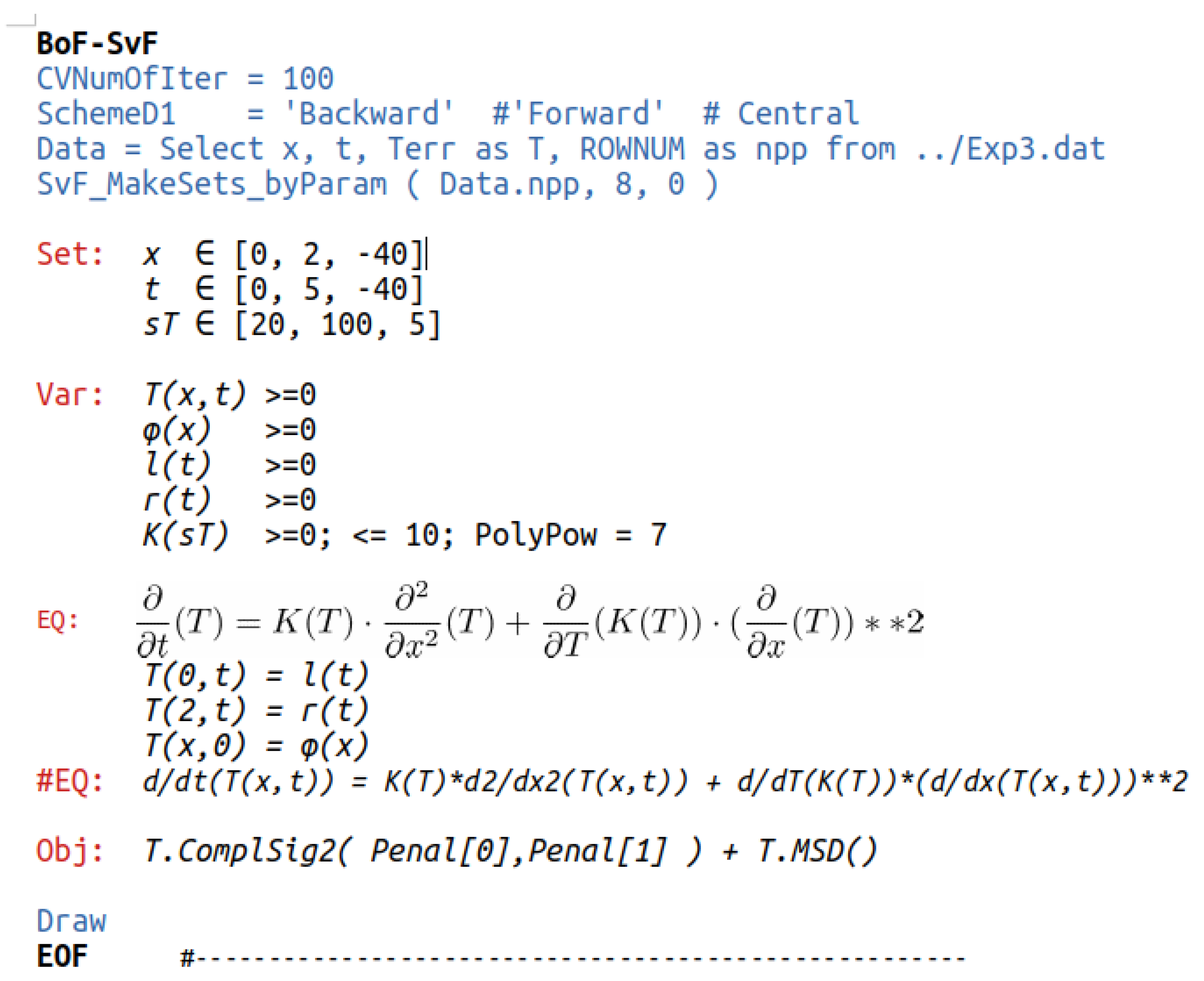
2]). At the user level, an expert (with knowledge about the object under study) prepares data files and a task file. The data files contain tables with experimental data (as plain text or in MS Excel or MS Access formats). The task file usually contains the data file names, a mathematical description of the object (formalization of the model in a notation close to mathematical, see
Appendix A), including a list of unknown parameters, as well as specifications of the cross-validation procedure (CV). These files are transferred to the client program, which replaces the variational problems with discrete ones, creates various sets (training and testing) for the CV procedure, formulates a number of NLP (nonlinear mathematical programming) problems and writes (formalizes) them in the Pyomo package language [
9]. The constructed data structures are transferred to a two-level optimization routine that implements an iterative numerical search for unknown model parameters and regularization coefficients to minimize the error of cross-validation. This subroutine can use the parallel solution of mathematical programming problems in a distributed environment of Everest optimization services [
10], namely SSOP applications [
11]. The Pyomo package converts the NLP description into so-called NL files, which are processed at the server level by special Ipopt solvers [
12]. The solutions are then collected and sent back to the client level and subsequently analyzed (for example, complete iterative process conditions are checked). If the iterative process is completed, the program prepares the results (calculates errors, creates solution files, draws graphs of the functions found) and presents them to the researcher (who may not know about the long chain of the tasks preceding the result).
The experts then utilize the results (especially the values of modeling errors–root-mean-square errors of cross validation) for choosing a new (or modified) model or deciding to cease calculations.
The software package together with examples (including some examples of this article) is freely available online (file SvF-2021-11.zip in the Git repository
https://github.com/distcomp/SvF, accessed on 1 September 2022).
SvF technology has been successfully applied in various scientific fields (mechanics, plasma physics, biology, plant physiology, epidemiology, meteorology, atmospheric pollution transfer, etc., and a more detailed enumeration can be found in [
2]) as an inverse problem solving method. In these studies, the main attention was paid to the construction of object models using specific regularization methods. This article, in contrast, focuses on the study of the regularization methods themselves, and the problem of heat conduction is chosen as a convenient example.
The problem of thermal conductivity is chosen to illustrate the technology. This is a classic problem in mathematical physics. It is well studied, and the one-dimensionality allows you to present the results in the form of graphs. Literature reviews can be found in [
7,
8]. The main task is to find the dependence of the thermal conductivity coefficient on temperature based on an array of experimental data. In total, nine problems were considered, differing in data sets and criteria for choosing solutions. Some of them are original. This is the first time such a comprehensive study with error analysis has been carried out. Various estimates of the modeling errors are given and turn out to be in good agreement with the characteristics of the synthetic data errors.
3. Data Sets
Formalizing the concept of a data set (observations or measurements set):
where
Ti is the temperature measurement at point
xi at time
ti.
For vectors of dimension
ǀDǀ, introduce the notation
Below, for numerical experiments, pseudo-experimental data are used, prepared on the basis of the exact solution (2) using pseudo-random number generators. The prepared 4 data sets were chosen as the most illustrative.
A basic data set was generated on a regular 11 × 11 grid (11 points in space 0, 0.2, 0.4 …, 2 and 11 points in time 0, 0.5, 1, … 5)
where
Ts(
xi,ti) are the values of the exact solution,
εi is the random error with variance
To generate εi, a normal distribution random number generator (gauss (0.2)) with zero mean and variance equal to 2 (degrees) was used. As a result, the distribution εi was obtained with average md = −0.10 (degrees) and variance σd = 2.06 (degrees). These characteristics of errors are not used in calculations but are taken into account when considering the results.
By analogy, we introduce a data set of exact measurements:
Let us define a data set containing 121 points randomly distributed on the
x,t plane:
To do this, use uniform(a, b)—a generator of random numbers uniformly distributed over the interval (a,b). The obtained characteristics of the normal distribution of temperature measurements are: md = −0.19 (degrees) and σd = 2.14 (degrees).
Finally, let us define a data set containing 1000 points, distributed in a random way:
with the characteristics of the normal distribution of temperature measurements:
md = −0.02 (degrees) and
σd = 2.01 (degrees).
The location of the measurement points of the
D_reg11x11, D_rnd121 and
D_rnd1000 sets on the
x,
t plane can be seen in
Figure 2.
4. Method of Balanced Identification
The general problem is finding a function T(x,t) (and other functions of model (1)) that approximates the data set D and, possibly, satisfies additional conditions (for example, the heat equation). To formalize it, we define an objective function (or selection criterion), which is a weighted sum of two terms: one formalizing the concept of the proximity of the model trajectory to the corresponding observations, the other formalizing the concept of the complexity of the model, expressed in this case through the measure of curvature included in the statement of functions.
Let us introduce a measure of the proximity of the trajectory of the model to measurements (data set
D) or the approximation error:
where
is the number of elements of the set
D,
and a measure of curvature (complexity) of functions of one variable
where [
a, b] is the domain of the function
f(x), and two variables
The objective function is a combination of the measures introduced above. Let us give, as an example, the objective function
The second term is the regularizing addition that makes the problem (of the search for a continuous function) correct. The choice of its value determines the quality of the solution.
Figure 2 shows two unsuccessful options (A—weights that are too large, C—too small) and one successful (B—optimal weights chosen to minimize the cross-validation error).
Hereinafter, the following designations are used:
rmsd = ‖ Ti – T(xi,ti) ‖D – the standard deviation of the solution from the measurements;
rmsd* – standard deviation of the balanced solution from measurements;
Err(x,t) = T(x,t) − Ts(x,t) – deviation of the solution from the exact solution;
Δ = ‖ Err(xi,ti) ‖D – the standard deviation of the SvF solution from the exact solution;
Δ* – estimation of Δ;
– error (mean square error) of cross-validation,
where
is the solution obtained by minimizing the objective functional for given
α on the set
D without point (
xi,ti). A more detailed (and more general) description of the cross-validation procedure can be found in [
2].
An optimally balanced SvF solution is obtained by minimizing the cross-validation error by regularization coefficients (
α):
As a justification for using the minimization of
σcv to choose a model (regularization weights), we present the following reasoning (here (·
i) stands for (
xi,ti)):
The second term represents the sum of the products of random variables
εi by an expression in parentheses, with the value of
εi excluded from the calculation (point
i was removed from the data set). It is expected to tend to zero with an increase of the observations’ number. Similarly, with an increase of the observations’ number (everywhere dense in space (
x,t)), the third term tends to
Δ2, since
. As a result, we obtain the estimate
Thus, cross-validation error minimizing leads (if a number of observations go to infinity) to minimizing the deviation of the solution found from the (unknown) exact solution. To assess such a deviation, introduce the designation:
Remark. The payment for the problem regularization, as a rule, is the distortion of the solution. Moreover, the greater the weight of the regularization, the greater the distortion. In the case under consideration, the distortion consists in “straightening” the solution. The extreme case of “straightening” is shown in
Figure 2A.
5. Various Identification Problems and Their Numerical Solution
Nine different identification tasks are discussed below. They differ in choices of data sets, minimization criteria (various regularizing additives) and additional conditions. For example, in Problem 5.1
MSD(
D_reg11x11)
+ Curv(
T):
M = 0, the minimization criterion is used:
which means for the given regularization weights
αx,αt and a given data set
D_reg11x11, find a set of functions (
T,
K,
φ,
l,
r) that minimizes the functional
MSD(D_reg11x11,T) + Curv(T,αx,αt), and the sought functions must satisfy the equations of the model
M = 0. This criterion is used to minimize the error of cross-validation, which makes it possible to find the regularization weights and the corresponding balanced SvF solution (
T,
K,
φ,
l,
r).
To reduce the size of the formulas, a more compact notation for the selection criterion is used:
The same notation will be used for the other problems.
The mathematical study of the variational problems is not the subject of the article. Note that even the original inverse problems of this type can have a non-unique solution, in particular, there are different heat conductivity coefficients leading to the same solution
T(
x,t) [
7,
8]. Only Problem 5.0 (a spline approximation problem) is known to have a unique solution under rather simple conditions [
13].
To find approximate solutions, we will use numerical models, which are obtained from analytical ones by replacing arbitrary mathematical functions with functions specified on the grid or polynomials (only for
K(
T)), derivatives with their difference analogs, integrals with the sums. Note that the grid used for the numerical model (41 points in
x with a step equal to 0.05 and 21 points in
t with a step equal to 0.25) is not tied to the measurement points in any way. For simplicity (and stability of calculations), an implicit four-point scheme was chosen [
14]. The choice of scheme requires a separate study and is not carried out here. However, apparently, the optimization algorithm used for solving the problem as a whole (residual minimization) makes it possible to avoid a number of problems associated with the stability of calculations.
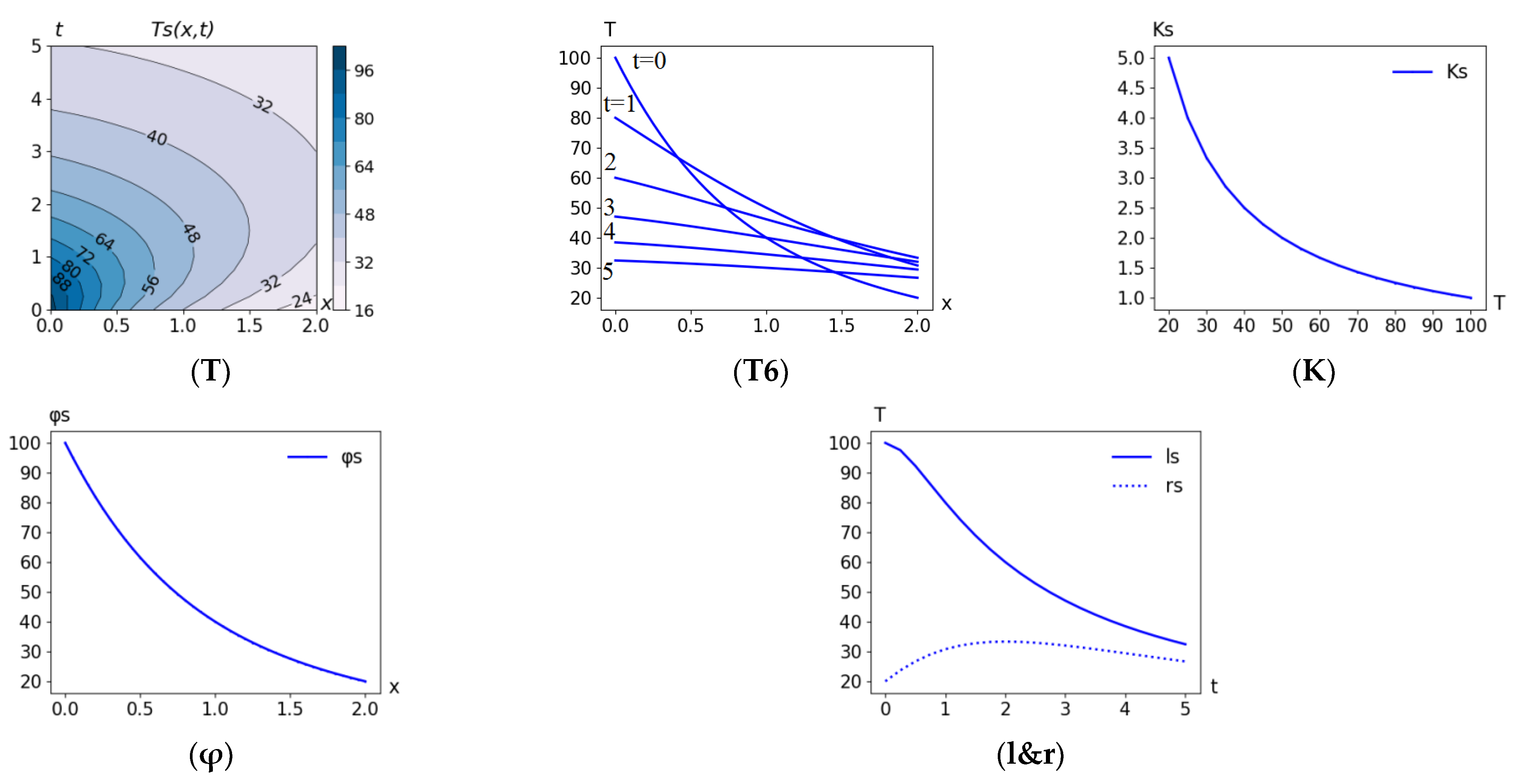
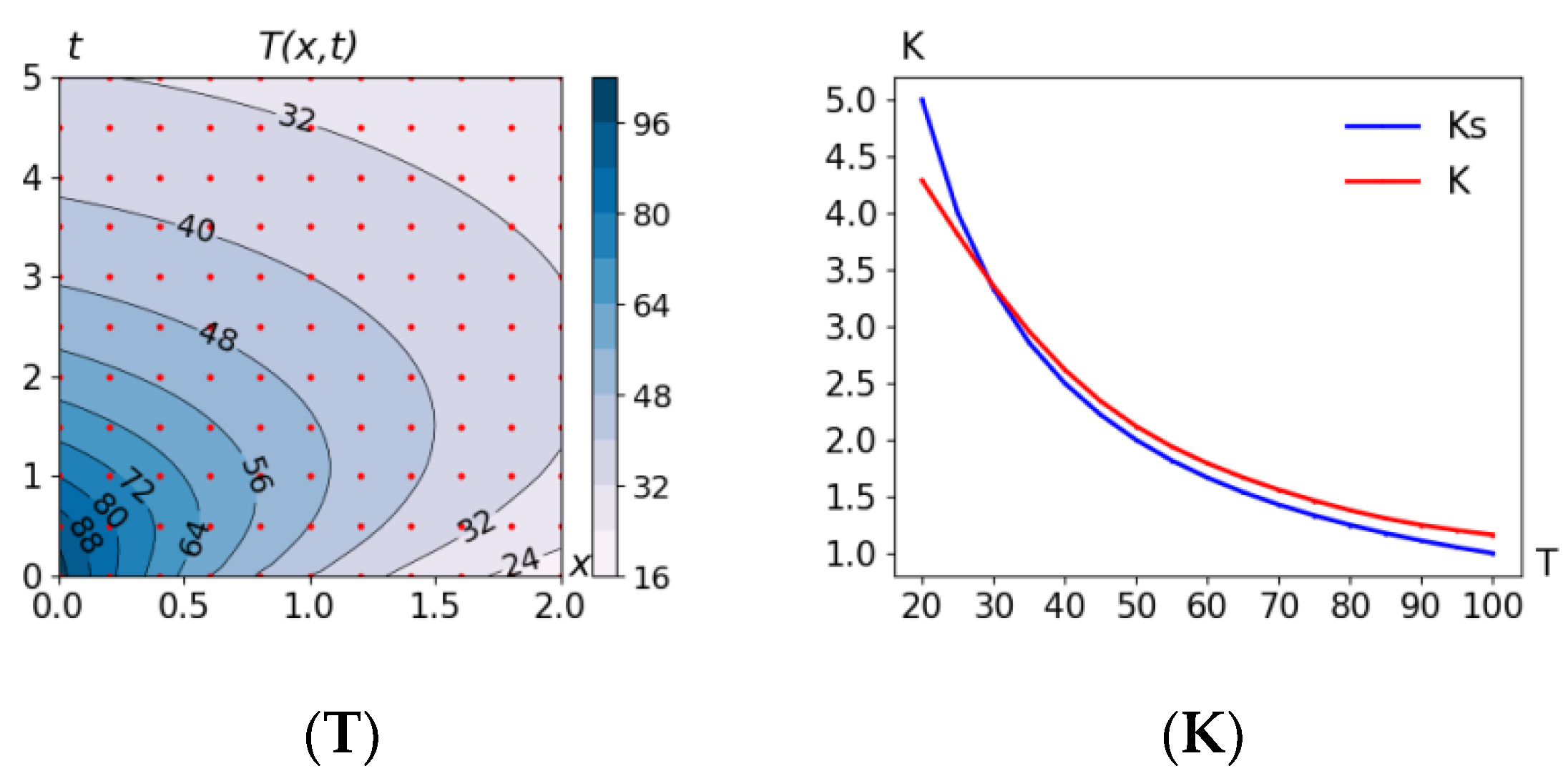
For the graphs of the exact solution, blue lines will be used, and for the SvF solution, red.
5.0. Problem MSD(D_reg11x11) + Curv(T)
Generally speaking, this simplest problem has nothing to do with the heat equation (therefore, its number is 0). It consists of finding a compromise between the proximity of the surface
T(
x,
t) to observations and its complexity (expressed in terms of the curvature
T(
x,
t)) based on the minimization functional:
The results of the numerical solution of the identification problem are shown in
Figure 3. The estimates obtained (resulting errors)
are benchmarks for assessing the errors of further problems.
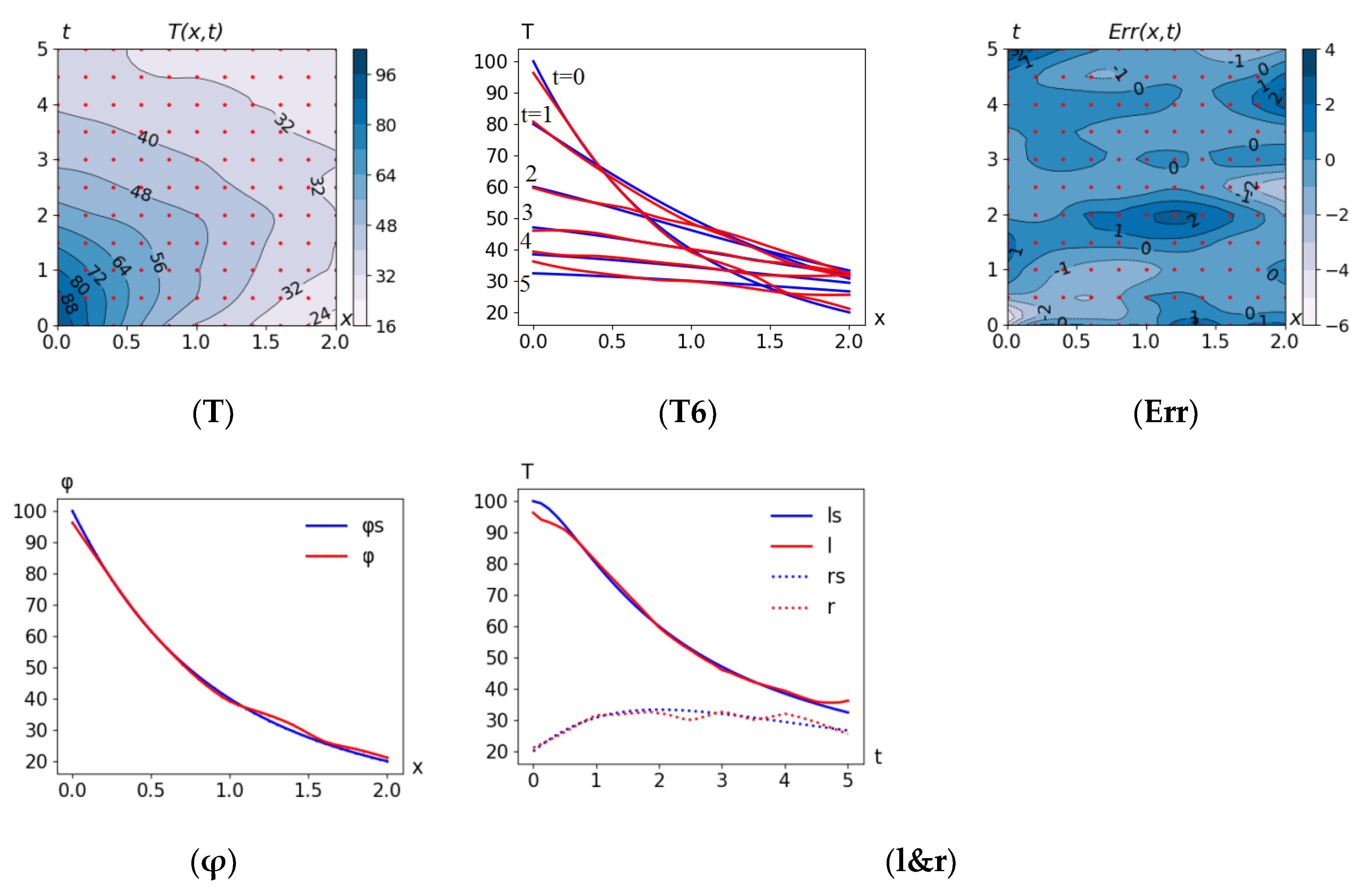
5.1. Problem MSD(D_reg11x11) + Curv(T): M = 0
Now, the identification problem is related to the heat conduction equation. It consists of minimizing the cross-validation error, provided that the solution sought satisfies the thermal conductivity equation (
M = 0), based on the criterion:
Errors: = 2.24, rmsd* = 1.58, Δ* = 0.86.
5.2. Problem MSD(D_reg11x11) + Curv(T): M = 0, l = ls, r = rs
Two additional conditions
l = ls, r = rs mean that the SvF solution must coincide with the exact one on the boundaries:
Here and below, the figures show not the entire set of functions, but only the essential ones (the rest do not change much). The results are shown in
Figure 5.
Errors: = 2.15, rmsd* = 1.86, Δ* = 0.61.
5.3. Problem MSD(D_reg11x11) + Curv(T): M = 0, l = ls, r = rs, φ = φs
Suppose that the initial condition is also known:
Errors: = 2.06, rmsd* = 2.01, Δ* = 0.49.
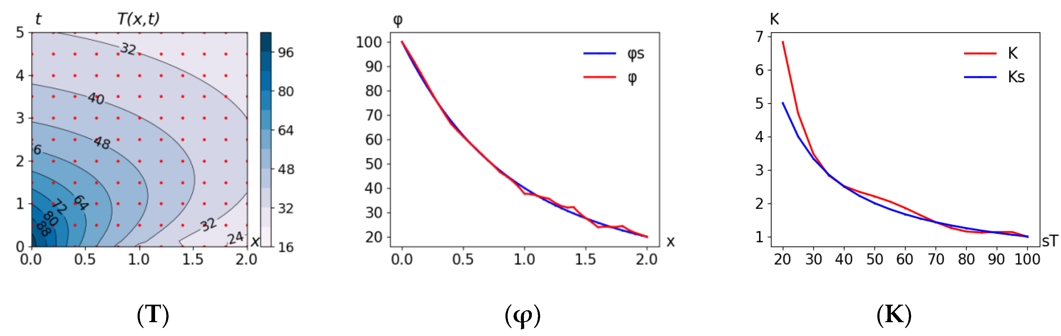
5.4. Problem MSD(D_reg11x11) + Curv(φ) + Curv(l) + Curv(r) + Curv(K):M = 0
The problem differs from Problem 5.1 by the penalties of four functions
φ, l, r and
K, that determine the solution, replacing the penalty for the curvature of the solution
T(x,t):
The formulation seems to be more consistent with the physics of the phenomenon—regularization occurs at the level of functions that determine the solution, and not at the solution itself.
Errors: = 2.22, rmsd* = 1.82, Δ* = 0.83.
Attention should be paid to the incorrect behavior of the thermal conductivity coefficient near the right border of the graph in
Figure 7K.
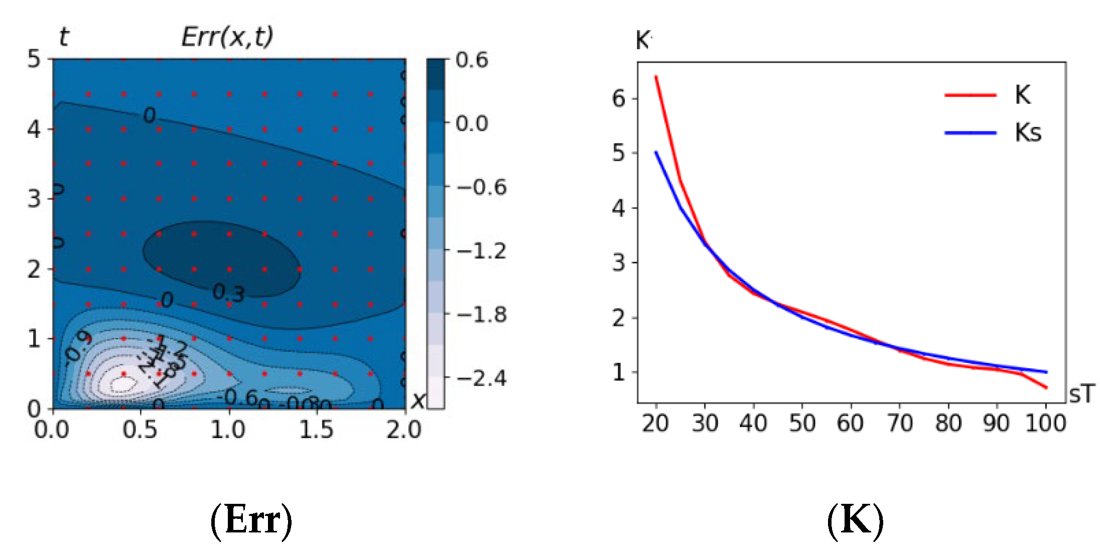
5.5. Problem MSD(D_reg11x11) + Curv(φ) +Curv(l) + Curv(r) + Curv(K): M = 0, dK/dT <= 0
Let it be additionally known that the thermal conductivity does not increase with increasing temperature
dK/dT <= 0:
This is an attempt to correct the solution by adding to the formulation of the minimization problem an additional condition formalizing a priori knowledge of the behavior of the coefficient
K(T) (see
Figure 7K and
Figure 8K).
Errors: = 2.23, rmsd* = 1.80, Δ* = 0.85.
5.6. Problem MSD(D_rnd121) + Curv(T): M = 0, l = ls, r = rs, φ = φs
The problem is similar to Problem 5.3, except the data set consists of 121 points on an irregular grid:
Errors: = 2.13, rmsd* = 2.05, Δ* = 0.39.
5.7. Problem MSD(D_rnd1000) + Curv(T): M = 0, l = ls, r = rs , φ = φs
The problem is similar to problem 5.6, except the data set consists of 1000 points:
Errors: = 2.02, rmsd* = 2.01, Δ* = 0.15.
5.8. Problem MSD(D_reg11x11(ε = 0)) + Curv(φ) + Curv(l) + Curv(r) + Curv(K):M = 0
The problem is similar to Problem 5.4, but with a set of exact measurements (
εi = 0):
Errors: = 0.06, rmsd* = 0.004, Δ* = 0.
The graphs of the boundary and initial conditions are not shown, since the SvF solutions actually coincide with the exact one.
6. Discussion
The errors obtained during problem solving are summarized in
Table 1. Analyzing the table allowed us to identify some of the patterns that appeared during problem modification.
Lines 0–3. Lines 0–3 of
Table 1 show some patterns of successive model modifications. As expected, adding the “correct” additional conditions leads to a more accurate (see column
Δ) modification of the model. These conditions reduce the set of feasible solutions of the optimization problem, while adding “correct” conditions cuts off unnecessary (non-essential) parts from it. In the technology used, this leads to a decrease in the
cross-validation error.
The growth of the
rmsd* error seems paradoxical: the more accurate the model, the greater its root mean square deviation from observations. However, it is easy to explain. First of all,
rmsd* is within the error limits of the initial data
σd. Second, the better the model, the closer it is to the exact solution, and for the exact solution
rmsd = σd. Of course, if regularization penalties that are too large are chosen, the solution will be distorted so that
rmsd will be greater than
σd. This situation is shown in
Figure 2A.
During modification, every subsequent model (from 0 to 3) is a follow up of the previous one. Previously found solutions are used as initial approximations, which allows us to find solutions faster as well as avoid poorly interpreted solutions.
Lines 4–5. The problems considered differ from Problem 5.1 by the selection criterion: instead of the solution T, the functions φ, l, r, and K (defining the solution) are used for regularization. This formulation seems to be more consistent with the physics of the phenomenon—a penalty imposed on the original functions determining the dynamics of the process, and not on their consequence (solution). The estimates of the cross-validation error (σcv) obtained are similar to Problem 5.1 but with smaller deviation from the exact solution Δ. The decrease in deviation may be associated with a special case of generated errors. The issue requires further research.
In Problem 5.4, the obtained solution of the thermal conductivity coefficient
K (T) (see
Figure 7K) rises sharply to the right border. Suppose it is known in advance that the coefficient is not to increase. This knowledge can be easily added to the model as an additional condition (
dK/dT <= 0). As a result (Problem 5.5),
K(T) changed (see
Figure 8K). At the same time, the accuracy indicators (line 5) practically stayed unchanged, which indicates that such an additional condition does not contradict the model and observations.
Line 6. Problem similar to Problem 5.3 but with a data set with a random arrangement of observations in space and time. The same number of observations leads to the same error estimates but the deviation from the exact solution is noticeably smaller. The use of such data sets should be carefully considered.
Line 7. Increasing the number of observations to 1000 significantly improves the accuracy of the solution.
Line 8. Using a data set with precise measurements allows us to get a close-to-exact solution.
General notes. The Δ* estimate generally describes Δ (the standard deviation of the SvF solution from the exact one) well enough. Note, that the data error σd (usually unknown) is used for the calculations.
Figure 4Err,
Figure 6Err,
Figure 8Err,
Figure 9T and
Figure 10Err show how the regularization distorts the solution. As expected, distortions are mainly observed in regions with high curvature (large values of the squares of the second derivatives).
It is easy to see that almost for all problems (except problem 5.8), the following inequalities hold:
It appears to be true when the model used, the regularization method, and the chosen cross-validation procedure are consistent with the data used and the physics of the phenomenon. At least, if the wrong model is chosen for describing the data (an incorrect mathematical description or too severe a regularization penalty), then the right-hand side of the inequality does not hold. If the errors in setting the data are not random (for example, space position related) or the cross-validation procedure is chosen incorrectly, the left side of the inequality will be violated. Thus, the violation of the inequality above is a sign of something going wrong.
7. Conclusions
The problems (and their solution) considered in the article illustrate the effectiveness of the application of regularization methods and, in particular, the use of balanced identification technology.
The results above confirm the thesis: the more data, the higher the accuracy, and the more knowledge about the object, the more complex and accurate models can be constructed. The technology used allows us to organize the evolutionary process of building models, from simple to complex. In this case, the indicator determining “the winner in the competitive struggle of models” is the error of cross-validation—reducing the error is a big argument in favor of this model.
In addition, this gradual (evolutionary) modification is highly desirable as the formulations under consideration are complex two-level (possibly multi-extreme) optimization problems and their solution requires significant resources. Thus, finding a solution without a “plausible” initial approximation would require computational resources that are too large and, in addition, one cannot be sure that the solution found (one of the local minima of the optimization problem) will have a subject interpretation that satisfies the researcher.
This step-by-step complication of the problem, together with specific techniques such as doubling the number of grid nodes, can significantly save computational resources. All of this work’s results were obtained on a modern laptop (CORE i5 processor) within a reasonable time (up to 1 h). The two-level optimization problem, which in this case allows parallelization, consumes the majority of the resources. Tools for the solution of more complex resource-intensive tasks exist for high-performance multiprocessor complexes [
10,
11].
As for computing resources, SvF technology is resource intensive. This is justified as it is aimed at saving the researcher’s time.
Appendix A contains a listing of the task file. The notation used is close to the mathematical one—a formal description of the model for calculations practically coincides with the formulas of the model (1). This allows for an easy model modification (no “manual” program code rewriting). For example, to take into account the heat flux at the border, a corresponding condition defining the derivative at the border has to be added to the task file.
Let us take a look at unsolved problems and possible solutions.
One problem is possible local minima. However, there are special solvers designed to search for global extrema, for example, SCIP [
15] (source codes are available) which implements the branch-and-bound algorithm, including global optimization problems with continuous variables. Perhaps, if a previously found solution is used as an initial approximation, a confirmation that the found minimum is global might be obtained in a reasonable time.
Finally, the paper considers various errors’ estimates of solution T(x,t) only and not the other functions’ identification accuracy. The evaluation of the accuracy of determining the thermal conductivity coefficient is particularly interesting. Another problem is the formalization of errors that arise when replacing a real physical object with a mathematical model and real observations with a measurement error model. In the future, these issues should be researched.


