Studies of the Fractional Selkov Dynamical System for Describing the Self-Oscillatory Regime of Microseisms

Abstract

A non-linear fractional Selkov dynamic system for mathematical modeling of microseismic phenomena is proposed. This system is a generalization of the previously known Selkov system, which has self-oscillatory modes and is used in biology to describe glycolytic vibrations of the substrate and product. The Selkov fractional dynamical system takes into account the influence of heredity and is described using derivative fractional orders. The article investigates the Selkov fractional dynamic model using the Adams–Bashforth–Moulton numerical method, constructs oscillograms and phase trajectories, and studies the equilibrium points. Based on the spectra of the maximum Lyapunov exponents, it is shown that in the fractional dynamic model there can be relaxation and damped oscillations.

1. Introduction

Microseisms are oscillations of the earth’s surface of small amplitude, the source of which are natural and man-made processes. In particular, processes in the atmosphere (cyclones), the impact of the seas and oceans on the coast, and processes associated with human activity (construction of buildings and structures). For the occurrence of microseisms in the zones of the earth’s crust, the presence of media is necessary, which, on the one hand, can accumulate stresses, which is associated with elasticity, and on the other hand, have the property of fragility, i.e., the ability to collapse under the influence of forces, the level of which is noticeably below the yield strength [1]. The fragility of the medium is realized at the macroscopic level due to the appearance and growth of the length of cracks. The process of multiple cracking ends with the destruction (loss of integrity) of the object under study. In this work, we will investigate the process of crack formation at an early stage of fracture.

It should be noted that cracks may not develop over time, and taking into account the viscosity of the medium, some cracks may even heal. Such a process, according to the authors of the article [2], can occur in the Earth’s crust at depths where there is high pressure and temperature, which contribute to the diffusion process at the tips of the cracks, which leads to the tightening of the cracks.

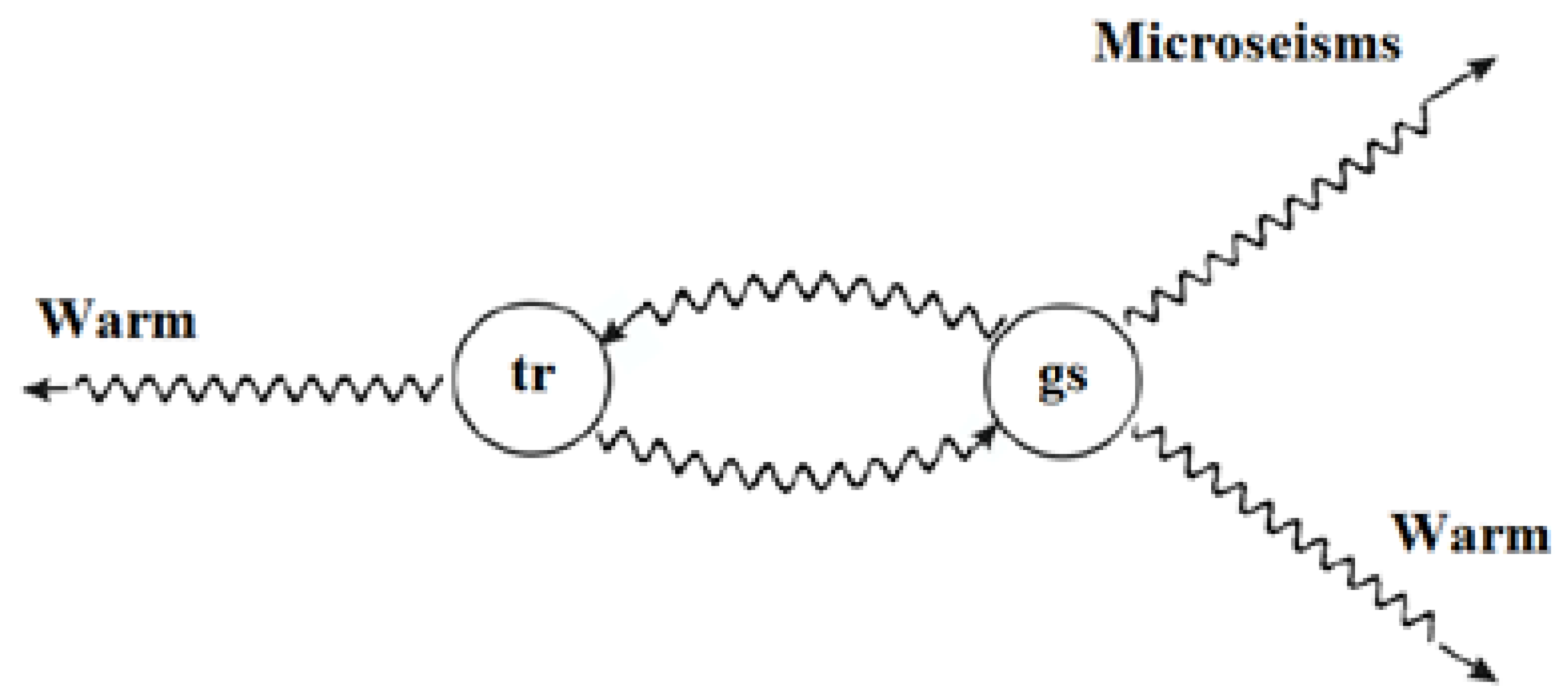
Microseisms can be divided into two types: microseisms of the first and second types. Microseisms of the first type are regular weak oscillations with a period of 2 to 10 s. Microseisms of the second type are less regular with a longer oscillation period up to 30 s [2]. Microseisms of the first kind are excited by cracks of small length, which are not recorded by seismic equipment. We will call such cracks tr-cracks; they are triggers for larger cracks. Microseisms of the second kind are excited by cracks of greater length, which are already recorded by seismic equipment. We will call these cracks gs-cracks.

In this work, we will investigate the mechanism of self-oscillations of microseismic sources or fluctuations in the concentration of gs-cracks by analogy with [2].

The self-oscillatory process here consists in the interaction between tr-cracks and gs-cracks (Figure 1).

The first type of cracks are seed cracks with lower energy and, when the critical concentration level is reached, it passes into the second type. Cracks of the second type are a source of microseismic phenomena (oscillations) and, after the release of their energy, they partially disappear and partially pass into seed cracks (the Le Chatelier–Brown principle, [3]). Further, this self-oscillatory process is repeated.

In the article [2], the authors proposed an interesting approach to describing the self-oscillating process during the interaction of cracks in an elastic-brittle medium, which is based on the use of the Selkov nonlinear dynamic system, which is studied in the framework of biology [4].

In this paper, we consider a generalization of the Selkov dynamic system to the case where the effect of hereditarity is taken into account. Hereditary means that the system can “remember” the impact on it for some time. Hereditarity effects were first considered within the framework of hereditary mechanics to describe viscoelastic or plastic media [5].

The effects of heredity are described in terms of integro-differential equations of the Volterra type. The integrands of these equations contain difference kernels or “memory” functions [6]. Memory functions are selected based on experimental data, properties of the medium or the process under consideration. However, memory functions are often chosen to be power-law to describe the influence of heredity, which diminishes over time, and power-laws are common in our environment. Power memory functions allow using the mathematical apparatus of fractional calculus and moving from integro-differential equations to equations with fractional derivatives [7,8,9].

Dynamical systems, which are described with the help of derivatives of fractional orders, are called fractional dynamical systems or dynamical systems of fractional order [10]. Fractional dynamical systems have applications in various fields of knowledge. For example, they are used in describing financial systems [11], in image encryption problems [12], in various discrete and continuous dynamic systems in the study of chaotic and regular modes [13,14,15], in synchronization problems in electrical circuits [16], etc.

Due to the fact that it is necessary to study the self-oscillating nature of the interaction of cracks of two types, the main purpose of this article is to conduct a qualitative analysis with the aim of: studying the equilibrium points of the Selkov fractional dynamic system in commensurate and incommensurable cases, studying regular and chaotic modes using spectra of maximum Lyapunov exponents (MLEs) to confirm the results obtained by constructing waveforms and phase trajectories using the Adams–Bashforth–Moulton (ABM) numerical algorithm. The results obtained confirm the possibility of the existence of self-oscillating regimes within the framework of the fractional Selkov dynamical system (FSDS). FSDS is a generalization of the classical Selkov dynamical system (CSDS), a qualitative analysis of which is given in [17].

The research plan in the article has the following structure: the introduction reveals the problems of the article, Section 2 provides some elements of the fractional calculus necessary for further research, Section 3 reveals the formulation of the problem, Section 4 deals with the asymptotic stability of fixed points, Section 5 gives a numerical Adams–Bashforth–Moulton method for solving the problem, in Section 6 examples of modeling and research of FSDS rest points are given, in Section 7 chaotic and regular modes of FSDS are studied using the construction of spectra of Lyapunov exponents, and in Section 8 conclusions are given on the results of the study.

2. Some Information from the Theory of Fractional Calculus

In this paragraph, we will consider the main definitions from the theory of fractional calculus, its aspects can be studied in more detail in the books [7,8,9].

Definition 1. 

Fractional Riemann–Liouville integral of order α:

$$I_{0t}^{\alpha }x\left(t\right)=\frac{1}{\Gamma \left(\alpha \right)}\underset{0}{\overset{t}{\int }}\frac{x\left(\tau \right)d\tau }{{\left(t-\tau \right)}^{1-\alpha }},\alpha >0,t>0,$$

(1)

where $\Gamma \left(·\right)$—gamma-function.

The fractional Riemann–Liouville integral (1) has the following properties:

$$I_{0t}^{0}x\left(t\right)=x\left(t\right),I_{0t}^{\alpha }{I}_{0t}^{\beta }x\left(t\right)=I_{0t}^{\alpha +\beta }x\left(t\right),I_{0t}^{\alpha }{I}_{0t}^{\beta }x\left(t\right)=I_{0t}^{\beta }{I}_{0t}^{\alpha }x\left(t\right).$$

Definition 2. 

The Gerasimov–Caputo fractional derivative of order α has the form:

$${\partial }_{0t}^{\alpha }x\left(t\right)=\left\{\begin{array}{c}{\displaystyle \frac{1}{\Gamma \left(m-\alpha \right)}}\underset{0}{\overset{t}{\int }}{\displaystyle \frac{x^{\left(m\right)}\left(\tau \right)d\tau }{{\left(t-\tau \right)}^{\alpha +1-m}}},0\le m-1<\alpha <m,\hfill \\ {\displaystyle \frac{d^{m}x\left(t\right)}{d{t}^m}},m\in N.\hfill \end{array}\right.$$

(2)

Operator (2) has the following properties:

$${\partial }_{0t}^{\alpha }{I}_{0t}^{\alpha }x\left(t\right)=x\left(t\right),I_{0t}^{\alpha }{\partial }_{0t}^{\alpha }x\left(t\right)=x\left(t\right)-{\displaystyle \sum _{k=0}^{i-1}}\frac{x^{\left(k\right)}\left(0\right)t^k}{k!},t>0.$$

3. Statement of the Problem

Consider the following nonlinear CSDS:

$$\left\{\begin{array}{c}\dot{x}\left(t\right)=-x\left(t\right)+ay\left(t\right)+b{x}^2\left(t\right)y\left(t\right),x\left(0\right)=x_0,\hfill \\ \dot{y}\left(t\right)=v-ay\left(t\right)-b{x}^2\left(t\right)y\left(t\right),y\left(0\right)=y_0,\hfill \end{array}\right.$$

(3)

where: $x\left(t\right)\in C^1\left[0,T\right]$—a function that determines the concentration of tr-cracks; $y\left(t\right)\in C^1\left[0,T\right]$—a function that determines the concentration of gs-cracks; $t\in \left[0,T\right]$—time of the process; $T>0$—simulation time; $x_0,y_0,v,a,b$— given positive constants; $\dot{x}\left(t\right)={\displaystyle \frac{dx}{dt}},\dot{y}\left(t\right)={\displaystyle \frac{dy}{dt}}$.

Remark 1. 

Note that system (3) was proposed by E.E. Selkov in [4] to describe the glycolytic reaction, which describes the self-oscillatory process of the substrate and product.

In this paper, we consider a generalization of the Cauchy problem (3) in the case when the system has memory. To do this, we will move from integer derivatives to derivatives of fractional orders in the sense of Gerasimov–Caputo (2):

$${\displaystyle \frac{d}{dt}}\to {\displaystyle \frac{1}{{\sigma }^{1-{\alpha }_1}}}{\partial }_{0t}^{{\alpha }_1},{\displaystyle \frac{d}{dt}}\to {\displaystyle \frac{1}{{\sigma }^{1-{\alpha }_2}}}{\partial }_{0t}^{{\alpha }_2},$$

where $\sigma$ has the dimension of time and $0<{\alpha }_1,{\alpha }_2<1$.

$$\left\{\begin{array}{c}{\partial }_{0t}^{{\alpha }_1}x\left(t\right)=-k_{1}x\left(t\right)+a_{1}y\left(t\right)+b_1{x}^2\left(t\right)y\left(t\right),x\left(0\right)=x_0,\hfill \\ {\partial }_{0t}^{{\alpha }_2}y\left(t\right)=v_0-a_{2}y\left(t\right)-b_2{x}^2\left(t\right)y\left(t\right),y\left(0\right)=y_0,\hfill \end{array}\right.$$

(4)

where $k_1={\sigma }^{1-{\alpha }_1},k_2={\sigma }^{1-{\alpha }_2},a_1=k_{1}a,b_1=k_{1}b,v_0=k_{2}v,a_2=k_{2}a,b_2=k_{2}b$.

Remark 2. 

The existence and uniqueness of the solution of fractional dynamical systems of type (4) is studied in the article [18].

The purpose of research in this paper is to study FSDS (4) for given values of parameters $x_0,y_0,v_0,a_1,b_1,a_2,b_2,{\alpha }_1,{\alpha }_2$—study of equilibrium points, construction of bifurcation diagrams, phase trajectories, and oscillograms, which should reveal regular and chaotic regimes.

Before proceeding to the study of self-oscillating regimes of the FSDS system (4), we give the key theorems on the asymptotic stability of equilibrium points for a commensurate and incommensurate dynamical system, as well as criteria for the existence of a chaotic regime and a closed phase trajectory [19].

4. Study of Equilibrium Points

Definition 3. 

If in the FSDS system (4) the orders of fractional derivatives are equal $\left({\alpha }_1={\alpha }_2=\alpha \right)$, then the system is commensurable. Otherwise, the FSDS (4) is said to be incommensurable.

Definition 4. 

Commensurable FSDS (4) has one equilibrium point $E=\left(x^{*},y^{*}\right)$:

$$x^{*}=v,y^{*}=\frac{v}{a+b{v}^2}.$$

(5)

which is a solution to the system for $k_1=k_2=k,a_1=a_2=a,b_1=b_2=b$:

$$\left\{\begin{array}{c}-kx\left(t\right)+ay\left(t\right)+b{x}^2\left(t\right)y\left(t\right)=0,\hfill \\ v_0-ay\left(t\right)-b{x}^2\left(t\right)y\left(t\right)=0.\hfill \end{array}\right.$$

Remark 3. 

Note that the Jacobi matrix for the commensurate FSDS system (4) has the form:

$$J\left(x,y\right)=\left(\begin{array}{cc}-\left(k-2bxy\right)& a+b{x}^2\\ -2bxy& -\left(a+b{x}^2\right)\end{array}\right).$$

(6)

and taking into account the equilibrium point (5), the Jacobi matrix (6) takes on a more specific form:

$$J\left(x^{*},y^{*}\right)=\left(\begin{array}{cc}{\displaystyle \frac{2b{v}^2-k(b{v}^2-a)}{a+b{v}^2}}& a+b{v}^2\\ {\displaystyle \frac{-2b{v}^2}{a+b{v}^2}}& -\left(a+b{v}^2\right)\end{array}\right).$$

(7)

Definition 5. 

Incommensurable FSDS (4) has one equilibrium point $E=\left(x^{*},y^{*}\right)$, which is the solution of the algebraic system:

$$\left\{\begin{array}{c}-k_{1}x\left(t\right)+a_{1}y\left(t\right)+b_1{x}^2\left(t\right)y\left(t\right)=0,\hfill \\ v_0-a_{2}y\left(t\right)-b_2{x}^2\left(t\right)y\left(t\right)=0.\hfill \end{array}\right.$$

Remark 4. 

Note that taking the Jacobi matrix into account the equilibrium point for the incommensurable FSDS (4) has the form:

$$J\left(x^{*},y^{*}\right)=\left(\begin{array}{cc}-\left(k_1-2b_1{x}^{*}{y}^{*}\right)& a_1+b_1{x}^{*2}\\ -2b_2{x}^{*}{y}^{*}& -\left(a_2+b_2{x}^{*2}\right)\end{array}\right).$$

(8)

Let us examine the equilibrium point for asymptotic stability. To do this, we turn to the following theorems, whose proofs can be found in [10,20].

For a commensurable system FSDS (4), the following theorem holds.

Theorem 1. 

An equilibrium point (5) is asymptotically stable for a commensurate FSDS (4) if all eigenvalues ${\lambda }_i$ of its Jacobi matrix (7) satisfy the condition

$$\left|arg\left({\lambda }_i\right)\right|>\frac{\alpha \pi }{2},i=1,2.$$

(9)

Let m be the least common multiple of the denominators of the fractional orders ${\alpha }_1={\beta }_1/{\varphi }_1,{\alpha }_2={\beta }_2/{\varphi }_2,{\beta }_i,{\varphi }_i\in Z,i=1,2$.

Similarly, for the incommensurable case of FSDS (4), a theorem is given.

Theorem 2. 

The equilibrium point (5) is asymptotically stable for an incommensurable FSDS (4), where ${\alpha }_i=\frac{{\beta }_i}{m},i=1,2$ if all eigenvalues of the Jacobi matrix (8) satisfy the condition

$$\left|arg\left(\lambda \right)\right|>\frac{\gamma \pi }{2},\gamma =\frac{1}{m},$$

(10)

where λ are the roots of the characteristic equation:

$$det\left(diag\left[{\lambda }^{m{\alpha }_1}{\lambda }^{m{\alpha }_2}\right]-J\left(x^{*},y^{*}\right)\right)=0.$$

(11)

A corollary of Theorem 2 is the following proposition.

Proposition 1. 

(Existence of chaotic regimes [20]). If condition

$$M=\frac{\pi }{2m}-\underset{i}{min}\left(|arg\left({\lambda }_i\right)|\right)<0$$

(12)

is satisfied, then there are no chaotic regimes in the dynamical system.

5. Research Tool

As a tool for studying FSDS system, to construct its oscillograms and phase trajectories, we use a numerical algorithm based on predictor-corrector finite-difference schemes.

In this article, to obtain a numerical solution of the FSDS (4) system, the Adams-Bashworth-Moulton (ABM) method was used, which was studied in [21,22,23].

The ABM method can be applied to the numerical solution of fractional dynamical systems of the FSDS type. Taking into account the definitions of the operators (1) and (2) and their compositional properties, we construct a predictor-corrector scheme on a uniform grid.

Let us introduce grid functions $x_{n+1}^p,y_{n+1}^p$, $n=0,\dots ,N-1$, which are solutions of the system of algebraic equations (predictor formula):

$$\left\{\begin{array}{c}{x}_{n+1}^p=x_0+\frac{{\tau }^{{\alpha }_1}}{\Gamma \left({\alpha }_1+1\right)}{\displaystyle \sum _{j=0}^n}{\theta }_{j,n+1}^1\left(-x_j+a{y}_j+b{x}_j^2{y}_j\right),\hfill \\ y_{n+1}^p=y_0+\frac{{\tau }^{{\alpha }_2}}{\Gamma \left({\alpha }_2+1\right)}{\displaystyle \sum _{j=0}^n}{\theta }_{j,n+1}^2\left(v-a{y}_j-b{x}_j^2{y}_j\right),\hfill \\ {\theta }_{j,n+1}^i={\left(n-j+1\right)}^{{\alpha }_i}-{\left(n-j\right)}^{{\alpha }_i},i=1,2,\hfill \end{array}\right.$$

(13)

where functions $x_{n+1}^{},y_{n+1}^{}$ are solutions of the following system of algebraic solutions (corrector formula):

$$\left\{\begin{array}{c}{x}_{n+1}=x_0+\frac{{\tau }^{{\alpha }_1}}{\Gamma \left({\alpha }_1+2\right)}\left(\left(-x_{n+1}^P+a{y}_{n+1}^P+b{\left(x_{n+1}^P\right)}^2{y}_{n+1}^P\right)+{\displaystyle \sum _{j=0}^n}{\rho }_{j,n+1}^1\left(-x_j+a{y}_j+b{x}_j^2{y}_j\right)\right),\hfill \\ y_{n+1}=y_0+\frac{{\tau }^{{\alpha }_2}}{\Gamma \left({\alpha }_2+2\right)}\left(v-a{y}_{n+1}^P-b{\left(x_{n+1}^P\right)}^2{y}_{n+1}^P+{\displaystyle \sum _{j=0}^n}{\rho }_{j,n+1}^2\left(v-a{y}_j-b{x}_j^2{y}_j\right)\right),\hfill \end{array}\right.$$

(14)

where the weights in (13) are defined as follows:

$${\rho }_{j,n+1}^i=\left\{\begin{array}{c}{n}^{{\alpha }_i+1}-\left(n-{\alpha }_i\right){\left(n+1\right)}^{{\alpha }_i},j=0,\hfill \\ {\left(n-j+2\right)}^{{\alpha }_i+1}+{\left(n-j\right)}^{{\alpha }_i+1}-2{\left(n-j+1\right)}^{{\alpha }_i+1},1\le j\le n,\hfill \\ 1,,j=n+1,\hfill \\ i=1,2.\hfill \end{array}\right.$$

The ABM method has the following error estimate [23]:

$$\underset{1\le j\le k}{max}\left|x_i\left(t_j\right)-x_{i,j}\right|=O\left({\tau }^{1+\underset{i}{min}{\alpha }_i}\right),$$

where $x_{ij}$ is the numerical solution obtained by formula (14), $x_1\left(t_j\right)=x\left(t_j\right),x_2\left(t_j\right)=y\left(t_j\right)$, $i=1,2$.

Remark 5. 

It should be noted that in the case when ${\alpha }_i=1$ we obtain the well-known ABM method of the second order of accuracy.

The ABM method was implemented in the Maple2021 symbolic mathematics environment.

6. Research Results

In this section, we will show, using qualitative analysis and numerical simulation (ABM method), that self-oscillating modes are possible for FSDS (4) [24,25].

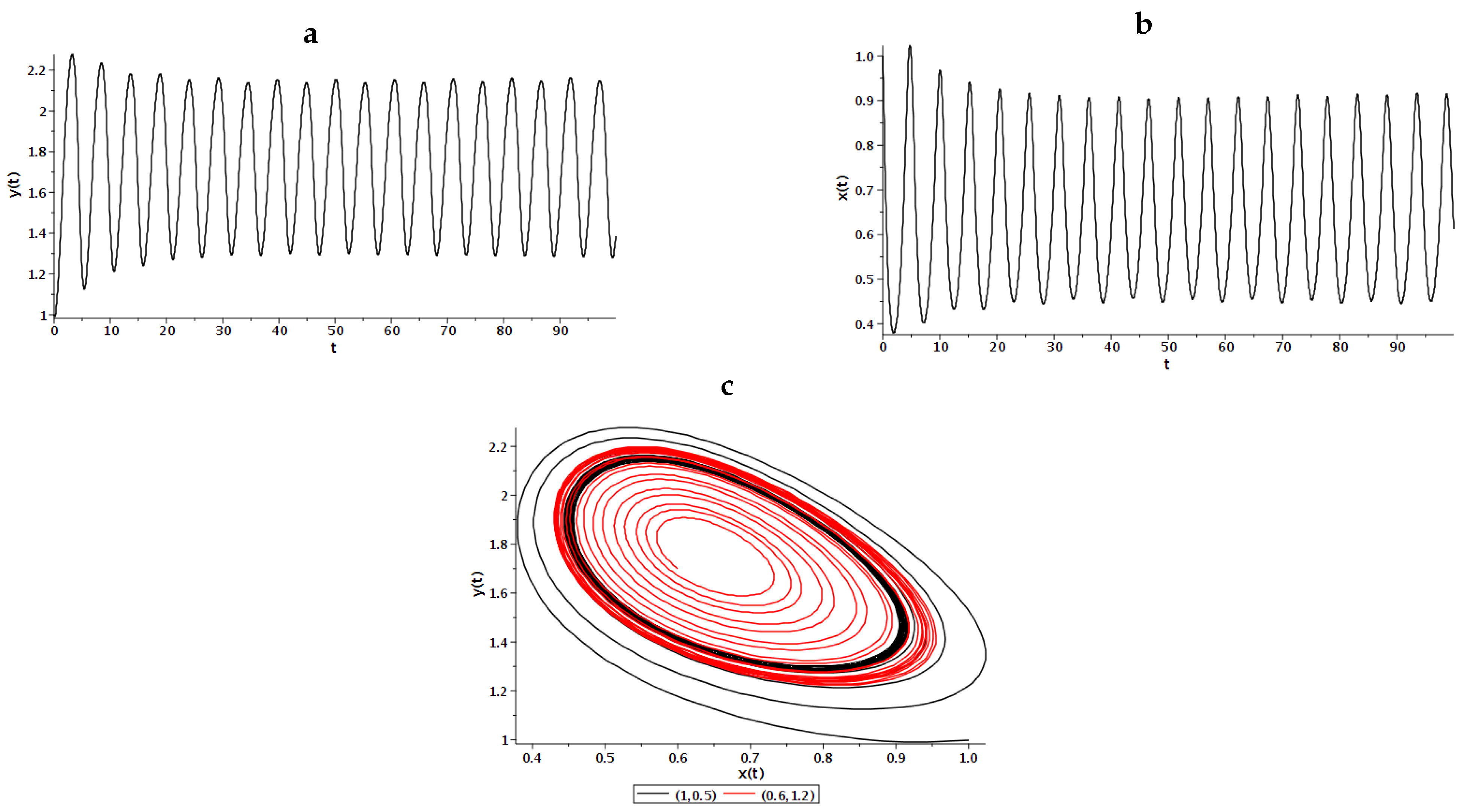
Example 1. 

(CSDS) If put in FSDS (4) ${\alpha }_1={\alpha }_2=\sigma =1$, then we come to a model CSDS [2]. The values of the parameters of system FSDS (4) are taken from the article [2]: $a=0.116,$$b=0.602, t\in \left[0,100\right]$. The values of the parameter $v=0.64421$ were chosen based on the fact that the trace of the Jacobi matrix is equal to zero in order for the limit cycle to exist.

In this case, the characteristic Equation (11) has purely imaginary roots: ${\lambda }_{1,2}=\pm 0.6048437164I$, so the equilibrium point can be the center or focus.

Therefore, the point of equilibrium $E=\left(0.6442125706,1.760933066\right)$ is the center.

A point of equilibrium of type center is stable, but not asymptotically stable. Indeed, according to Theorem 1, for a commensurate system (4) at ${\alpha }_1={\alpha }_2=1$, condition (9) is not satisfied. However, the phase trajectories in this case reach a stable limit cycle (Figure 2), as in [2].

Figure 2 shows the calculated curves of the oscillograms and phase trajectories obtained by method (13), (14) taking into account that $t\in \left[0,100\right]$ and the number of nodes of the computational $N=2000$. The initial conditions $\left(x_0,y_0\right)$ were chosen as follows: (1, 0.5)—black curve; (0.6, 1.2)—red curve.

This was done in order to show the stability of the limit cycle (Figure 2c) for Example 1. Indeed, we see that the phase trajectory highlighted in red, unwinding, tends to some limit trajectory. On the other hand, the phase trajectory, highlighted in black, also tends to this limiting trajectory. This limit trajectory is a stable cycle.

Consider an example in the case of a commensurate FSDS.

Figure 2. Oscillograms for the concentrations of gs-cracks (a) and tr-cracks (b); (c) phase trajectories constructed under different initial conditions for Example 1.

Figure 2. Oscillograms for the concentrations of gs-cracks (a) and tr-cracks (b); (c) phase trajectories constructed under different initial conditions for Example 1.

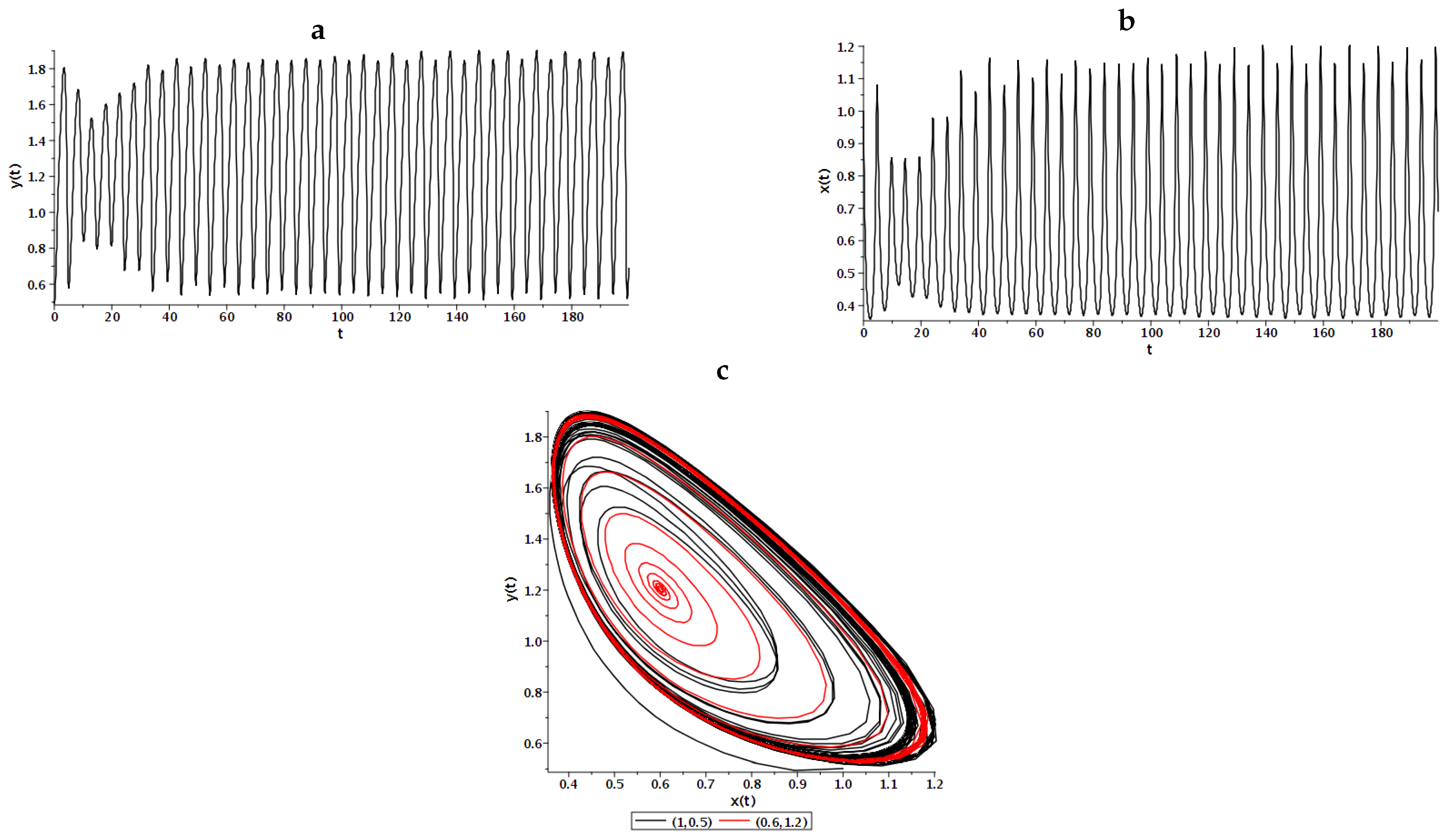
Example 2. 

(FSDS commensurable case). Let us consider the case of commensurable FSDS (4) with${\alpha }_1={\alpha }_2=0.8,\sigma =1$. We choose the parameter values $a=0.03, b=1.3, v=0.6$, $t\in \left[0,200\right]$, number of grid nodes $N=2000$. The equilibrium point in this case will have coordinates $E=\left(0.6,1.204819277\right)$.

According to Theorem 1, the characteristic equation for this point has the form:

$${\lambda }^{16}-0.3815180723{\lambda }^8+0.498=0,$$

whose roots satisfy condition (9). Indeed,

Table 1. Roots of the characteristic equation and their verification for condition (9).

No	Roots	Codition (9)
1	$0.9448075810-0.1545424593$I	True
2	$0.7773578684+0.5588018265$I	True
3	$0.1545424593+0.9448075810$I	True
4	$-0.5588018265+0.777357868$I	True
5	$-0.9448075810+0.154542459$I	True
6	$-0.7773578684-0.558801827$I	True
7	$-0.1545424593-0.94480758$I	True
8	$0.5588018265-0.7773578684$I	True
9	$0.9448075810+0.154542459$I	True
10	$0.5588018265+0.7773578684$I	True
11	$-0.1545424593+0.94480758$I	True
12	$-0.7773578684+0.55880183$I	True
13	$-0.9448075810-0.15454246$I	True
14	$-0.5588018265-0.77735787$I	True
15	$0.1545424593-0.9448075810$I	True
16	$0.7773578684-0.5588018265$I	True

shows all the roots of the characteristic equation with a condition check (9).

Therefore, the equilibrium point is asymptotically stable. The measure of the existence of chaotic modes is negative (12): $M=-0.0050548591<0$.

Based on the above, we can conclude that the system has a closed phase trajectory and does not have chaotic regimes. Due to the fact that the point is asymptotically stable, the closed trajectory is a stable limit cycle (Figure 3c).

As in the previous example, we see that the phase trajectory, highlighted in red, tends to some limit trajectory as it unwinds. At the same time, the phase trajectory, highlighted in black, also tends to this limiting trajectory.

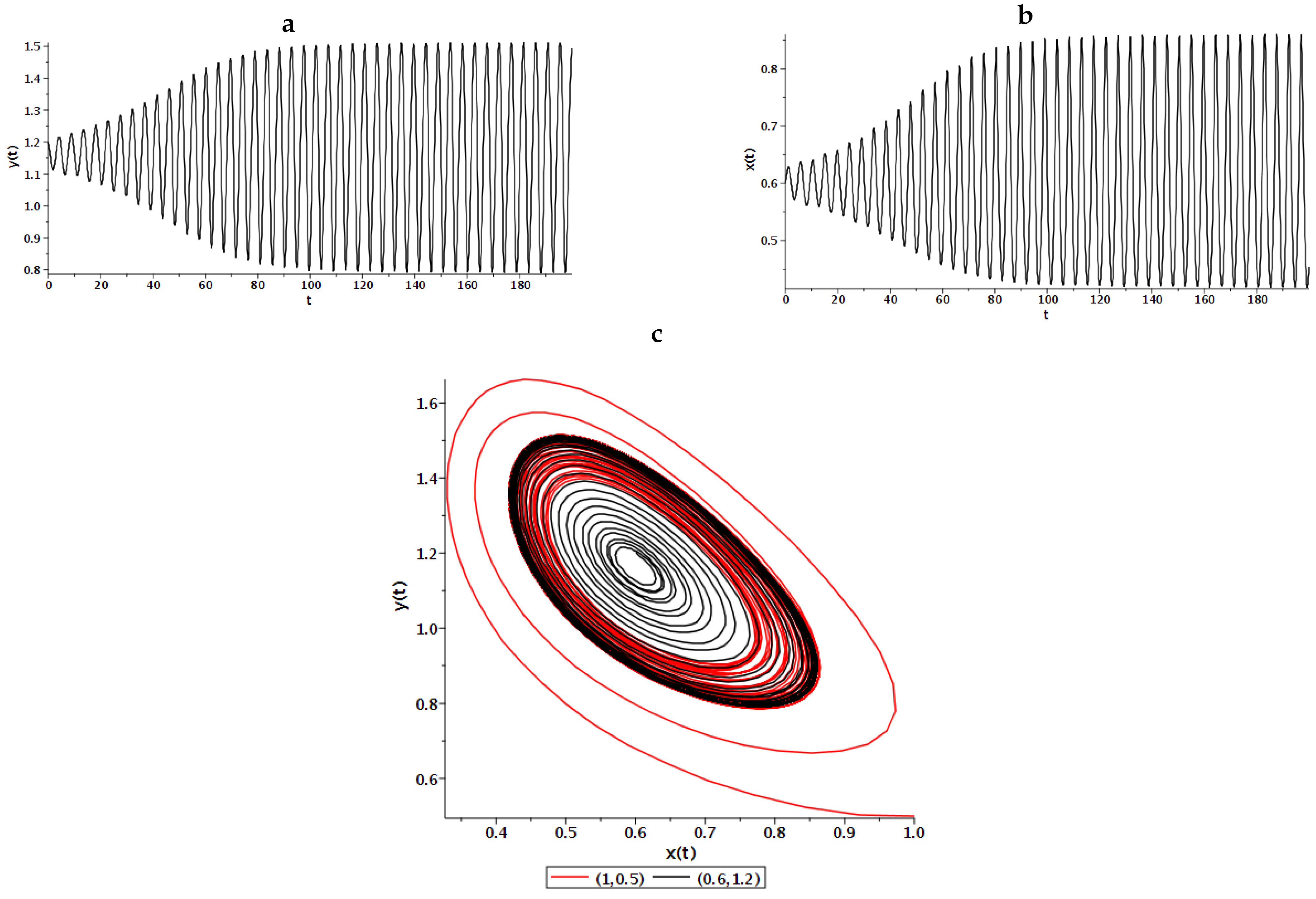
Example 3. 

(FSDS incommensurable case) Consider incommensurable FSDS (4) ${\alpha }_1=1,{\alpha }_2=0.9$; the rest of the parameter values will be chosen as follows $a=0.12,b=1.1,v=0.6,\sigma =1$.

Then the equilibrium point will have coordinates: $E=\left(0.6,1.162790698\right)$ Let us investigate this point for asymptotic stability.

According to Theorem 2, the characteristic Equation (11), taking into account the fact that ${\alpha }_1=\frac{10}{10},{\alpha }_2=\frac{9}{10}$, $m=10$, will take the form (8):

$${\lambda }^{19}-0.5348837209{\lambda }^{10}+0.516{\lambda }^9+0.516=0.$$

All roots of this equation satisfy condition (10) of Theorem 2, so the equilibrium point is asymptotically stable (Table 2).

According to the criterion for the existence of chaotic regimes for Example 3: $M=-0.0079816271<0$; therefore, they are absent.

Figure 4 shows the calculated curves of oscillograms and phase trajectories constructed by the ABM method (13), (14) at $N=2000,t\in \left[0,200\right]$. We see in Figure 4a,b that the oscillation amplitude increases to a certain constant level, which indicates the existence of a limit cycle. However, this cycle, as shown in Figure 4c, is unstable, since there are trajectories that repel from it (red curve).

Table 2. Roots of the characteristic equation and their verification for condition (10).

No	Roots	Codition (10)
1	$0.9587107281+0.1596989864$I	True
2	$0.8338678747+0.4505677490$I	True
3	$0.6751185224+0.7318032772$I	True
4	$0.3733655051+0.8484303397$I	True
5	$0.08517791582+1.011916745$I	True
6	$-0.222741495+0.8839001155$I	True
7	$-0.562141402+0.8623046746$I	True
8	$-0.711638255+0.5546773068$I	True
9	$-0.980118554+0.3368792296$I	True
10	$-0.8992016786$	True
11	$-0.980118554-0.3368792296$I	True
12	$-0.711638255-0.5546773068$I	True
13	$-0.562141402-0.8623046746$I	True
14	$-0.222741495-0.8839001155$I	True
15	$0.08517791582-1.011916745$I	True
16	$0.3733655051-0.8484303397$I	True
17	$0.6751185224-0.7318032772$I	True
18	$0.8338678747-0.4505677490$I	True
19	$0.9587107281-0.1596989864$I	True

Table 2. Roots of the characteristic equation and their verification for condition (10).

No	Roots	Codition (10)
1	$0.9587107281+0.1596989864$I	True
2	$0.8338678747+0.4505677490$I	True
3	$0.6751185224+0.7318032772$I	True
4	$0.3733655051+0.8484303397$I	True
5	$0.08517791582+1.011916745$I	True
6	$-0.222741495+0.8839001155$I	True
7	$-0.562141402+0.8623046746$I	True
8	$-0.711638255+0.5546773068$I	True
9	$-0.980118554+0.3368792296$I	True
10	$-0.8992016786$	True
11	$-0.980118554-0.3368792296$I	True
12	$-0.711638255-0.5546773068$I	True
13	$-0.562141402-0.8623046746$I	True
14	$-0.222741495-0.8839001155$I	True
15	$0.08517791582-1.011916745$I	True
16	$0.3733655051-0.8484303397$I	True
17	$0.6751185224-0.7318032772$I	True
18	$0.8338678747-0.4505677490$I	True
19	$0.9587107281-0.1596989864$I	True

7. Spectrum of Maximum Lyapunov Exponents

An analysis of the equilibrium points for FSDS (4) showed that the phase trajectories can reach a stable limit cycle. However, the question of the existence of chaotic regimes is also important, which we will try to investigate using the spectra of maximum Lyapunov exponents (MLEs), by analogy with the author’s works [25,26,27].

The MLE method is based on the study of perturbations in the trajectories of a dynamical system. Let $\Delta x\left(t\right)$, $\Delta y\left(t\right)$ be perturbations (variations) in coordinates $x\left(t\right)$ and $y\left(t\right)$ for FSDS (4). Let $f_1\left(x,t\right),f_2\left(x,t\right)$ be smooth functions right-hand sides of FSDS (4).

Definition 6. 

Equations in variations for FSDS (4) have the form:

$$\left\{\begin{array}{c}{\partial }_{0t}^{{\alpha }_1}\Delta x\left(t\right)=\Delta x\left(t\right)\frac{\partial f_1\left(x,y\right)}{\partial x}+\Delta y\left(t\right)\frac{\partial f_1\left(x,y\right)}{\partial y},\hfill \\ {\partial }_{0t}^{{\alpha }_2}\Delta y\left(t\right)=\Delta x\left(t\right)\frac{\partial f_2\left(x,y\right)}{\partial x}+\Delta y\left(t\right)\frac{\partial f_2\left(x,y\right)}{\partial y},\hfill \end{array}\right.$$

(15)

The system (15) can be rewritten in vector form:

$${\partial }_{0t}^{\alpha }\mathbf{v}\left(t\right)=J\left(x,y\right)\mathbf{v}\left(t\right),$$

where ${\partial }_{0t}^{\alpha }=\left\{{\partial }_{0t}^{{\alpha }_1},{\partial }_{0t}^{{\alpha }_2}\right\},\mathbf{v}\left(t\right)=\left\{\Delta x\left(t\right),\Delta y\left(t\right)\right\}.$

The vector $\mathbf{v}\left(t\right)$ is tangent to the trajectory of the original system (4). Depending on the direction of application of the perturbation and the properties of system (4), the vector $\mathbf{v}\left(t\right)$ can increase or decay due to linearity (15) according to a power law.

Remark 6. 

It should be noted that in the case of the CSDS model, the vector $\mathbf{v}\left(t\right)$ will decay or increase exponentially. In the case of FSDS, it can be shown that the analytical solutions of the system (15) are power functions of the Mittag–Leffler type, which, at values of parameters ${\alpha }_1={\alpha }_2=1$, turn into exponential functions.

Remark 7. 

For FSDS (4), the equations in variations (15) will take a specific form:

$$\left\{\begin{array}{c}{\partial }_{0t}^{{\alpha }_1}\Delta x\left(t\right)=\left(2b_{1}x\left(t\right)y\left(t\right)-k_1\right)\Delta x+\left(a_1+b_1{x}^2\left(t\right)\right)\Delta y,\hfill \\ {\partial }_{0t}^{{\alpha }_2}\Delta y\left(t\right)=-2b_{2}x\left(t\right)y\left(t\right)\Delta x+\left(-a_2-b_2{x}^2\left(t\right)\right)\Delta y.\hfill \end{array}\right.$$

(16)

System (16) is the key one for the MLE construction algorithm. Due to the fact that FSDS (4) consists of two equations, we can find at most two MLEs [28]. To find the MLE, we choose the Benettin–Wolf algorithm (BWA) [29,30].

Consider a BWA for two MLEs for the FSDS (4), which consists of the following stages:

1

We solve numerically the ABM method (13), (14), the original system (4) together with two sets of perturbed equations or equations in variations (16). As the initial vectors for the variational equations, it is necessary to choose a set of vectors ${\tilde{x}}_0^0,{\tilde{y}}_0^0$, which are orthogonal and normalized to unity.

2

In time T, the trajectory will come to a point—the vector $x_1$. We renormalize the perturbation vectors ${\tilde{x}}_1,{\tilde{y}}_1$ according to the Gram–Schmidt method using the formulas [31]: ${\tilde{x}}_1^0=\frac{{\tilde{x}}_1}{{∥{\tilde{x}}_1∥}_2},$${\tilde{y}}_1^0=\frac{{{\tilde{y}}^{\prime }}_1}{{∥{{\tilde{y}}^{\prime }}_1∥}_2},{\tilde{y}}_1^{\prime }={\tilde{y}}_1-\left({\tilde{y}}_1,{\tilde{x}}_1^0\right){\tilde{x}}_1^0.$ Here the notation $\left(,\right)$ is the scalar product of vectors.

3

We continue the calculation according to steps 1 and 2 from the perturbation vectors ${\tilde{x}}_1^0,{\tilde{y}}_1^0$. After a time interval T, we obtain a new set of perturbation vectors ${\tilde{x}}_2,{\tilde{y}}_2$, which are also subjected to the Gram–Schmidt orthogonalization procedure and further renormalization.

4

Steps 1–3 are repeated M times and the sums are calculated using the formulas:

$$S_1={\displaystyle \sum _{i=1}^M}ln\left({∥{\tilde{x}}_i∥}_2\right),S_2={\displaystyle \sum _{i=1}^M}ln\left({∥{\tilde{y}}_i∥}_2\right),$$

These formulas are calculated, in which the disturbance vectors appear before renormalization, but after orthogonalization.

5

MLEs are calculated with the formula:

$${\mathsf{\Lambda }}_{max}^i=\frac{S_i}{MT},i=1,\dots ,2.$$

Remark 8. 

Gram–Schmidt orthogonalization is necessary to eliminate the influence of the higher MLE component at large times when calculating vectors along the phase trajectory. Otherwise, the problem may be ill-conditioned.

It is important to study the MLE spectra, which are plotted depending on the parameter values of the FSDS model parameters (4) in case $\sigma =1$. The parameters for the system can be chosen as follows $v,a,b,{\alpha }_1,{\alpha }_2$.

Therefore, we will investigate the following dependences of the first MLE [28]: ${\mathsf{\Lambda }}_{max}\left(v\right)$, ${\mathsf{\Lambda }}_{max}\left(a\right)$, ${\mathsf{\Lambda }}_{max}\left(b\right)$, ${\mathsf{\Lambda }}_{max}\left({\alpha }_1\right)$, ${\mathsf{\Lambda }}_{max}\left({\alpha }_2\right)$. The second MLE usually has negative values, which indicates the absence of a chaotic regime.

Example 4. 

Let us construct bifurcation diagrams using the ABM method, taking into account the values of the parameters $v=0.5,a=0.1,b=\sigma =1,{\alpha }_2=1,t\in \left[0,100\right],x\left(0\right)=0.2,$$y\left(0\right)=0.3,$ with a step $\tau =0.05$.

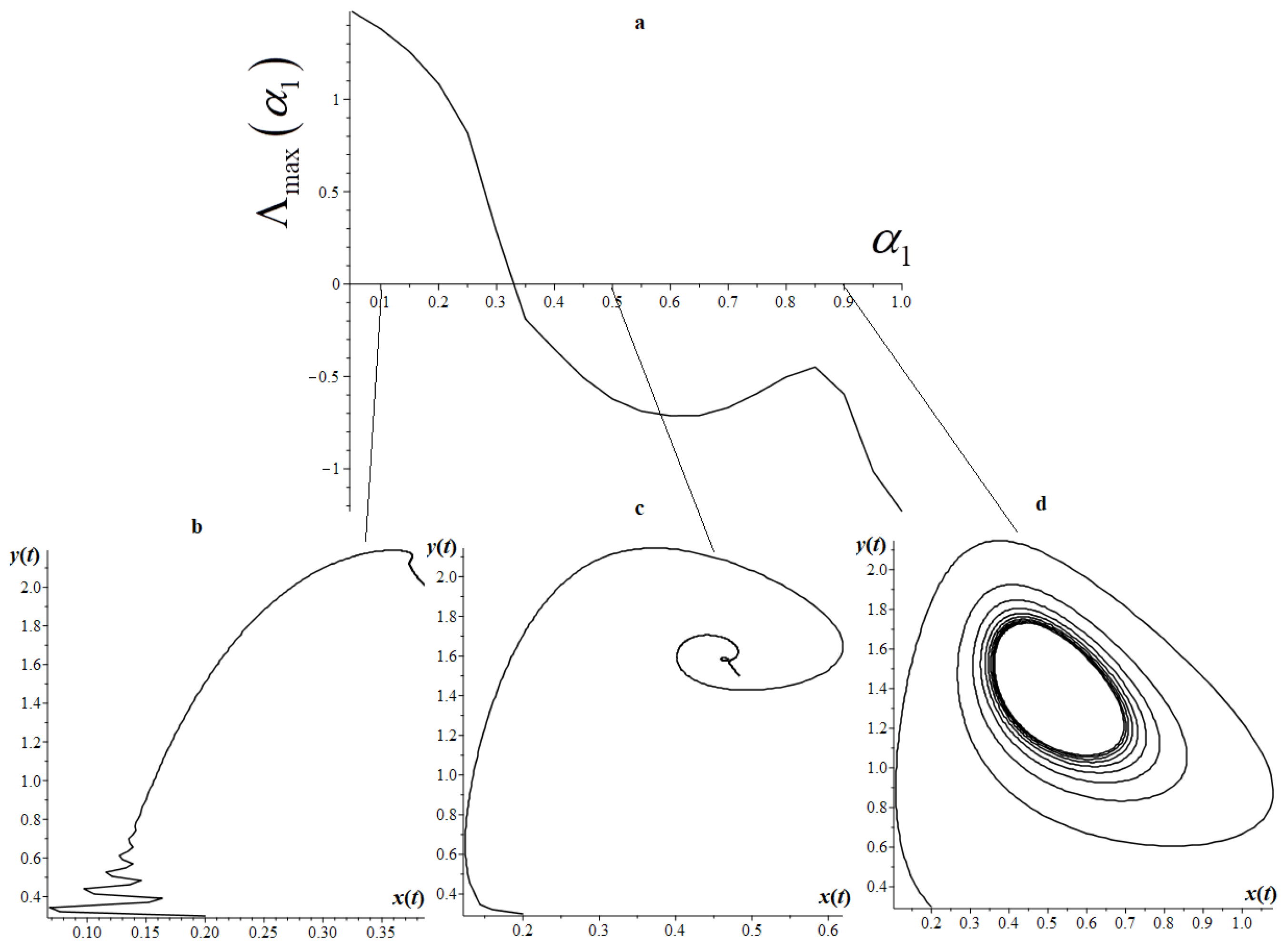
In Figure 5, we see that there are positive values in the MLE spectrum, which indicate the presence of a chaotic regime. Let us check if this fact really takes place in Example 4.

The MLE spectrum ${\mathsf{\Lambda }}_{max}\left({\alpha }_1\right)$ consists of positive values in the range of the parameter ${\alpha }_2\in \left[0,0.325\right)$ and negative values from the range ${\alpha }_2\in \left[0.325,1\right]$ (Figure 5).

Figure 5. (a)—Spectrum MLE ${\mathsf{\Lambda }}_{max}\left({\alpha }_1\right)$; (b)—phase trajectory for ${\alpha }_1=0.1$; (c)—phase trajectory for ${\alpha }_1=0.5$; (d)—phase trajectory for ${\alpha }_1=0.9$.

Figure 5. (a)—Spectrum MLE ${\mathsf{\Lambda }}_{max}\left({\alpha }_1\right)$; (b)—phase trajectory for ${\alpha }_1=0.1$; (c)—phase trajectory for ${\alpha }_1=0.5$; (d)—phase trajectory for ${\alpha }_1=0.9$.

Note that Figure 5 shows phase trajectories for different values of ${\alpha }_1$. At ${\alpha }_1=0.5$, the phase trajectory looks like a twisting spiral (stable focus) (Figure 5a); at ${\alpha }_1=0.9$, the phase trajectory is a limit cycle (Figure 5b). We are interested in the value ${\alpha }_1=0.1$, at which the MLE spectrum is positive. Here we have an open phase trajectory (Figure 5c). Does such a phase trajectory correspond to a chaotic regime? Let us use the criterion (12). In this case, $M<-0.1514163724$. This means that this mode is not chaotic. The phase trajectory corresponds to the aperiodic regime, i.e., damping process without hesitation.

Here, we observe the Andronov–Hopf bifurcation—the transition from a stable focus to a limit cycle at ${\alpha }_1\to 1$. The Andronov–Hopf bifurcation and the transition to the aperiodic regime indicate that the phase trajectories at ${\alpha }_1\to 0$ characterize the energy dissipation in the dynamical system. Here, ${\alpha }_1$ the order of the fractional derivative is related to the quality factor of the system by analogy with the results in [32], i.e., as the value of the order of the fractional derivative decreases, the limit cycle passes into a stable focus, and then we see damping without oscillations. Similarly, it can be shown that for the order ${\alpha }_2$ these conclusions remain valid.

Figure 5 shows that the graph of the function changes its sign when crossing zero. So there must be a limit cycle. We see from Figure 5b that there is a limit cycle. However, the limit cycle is destroyed when the ${\alpha }_1$ parameter changes.

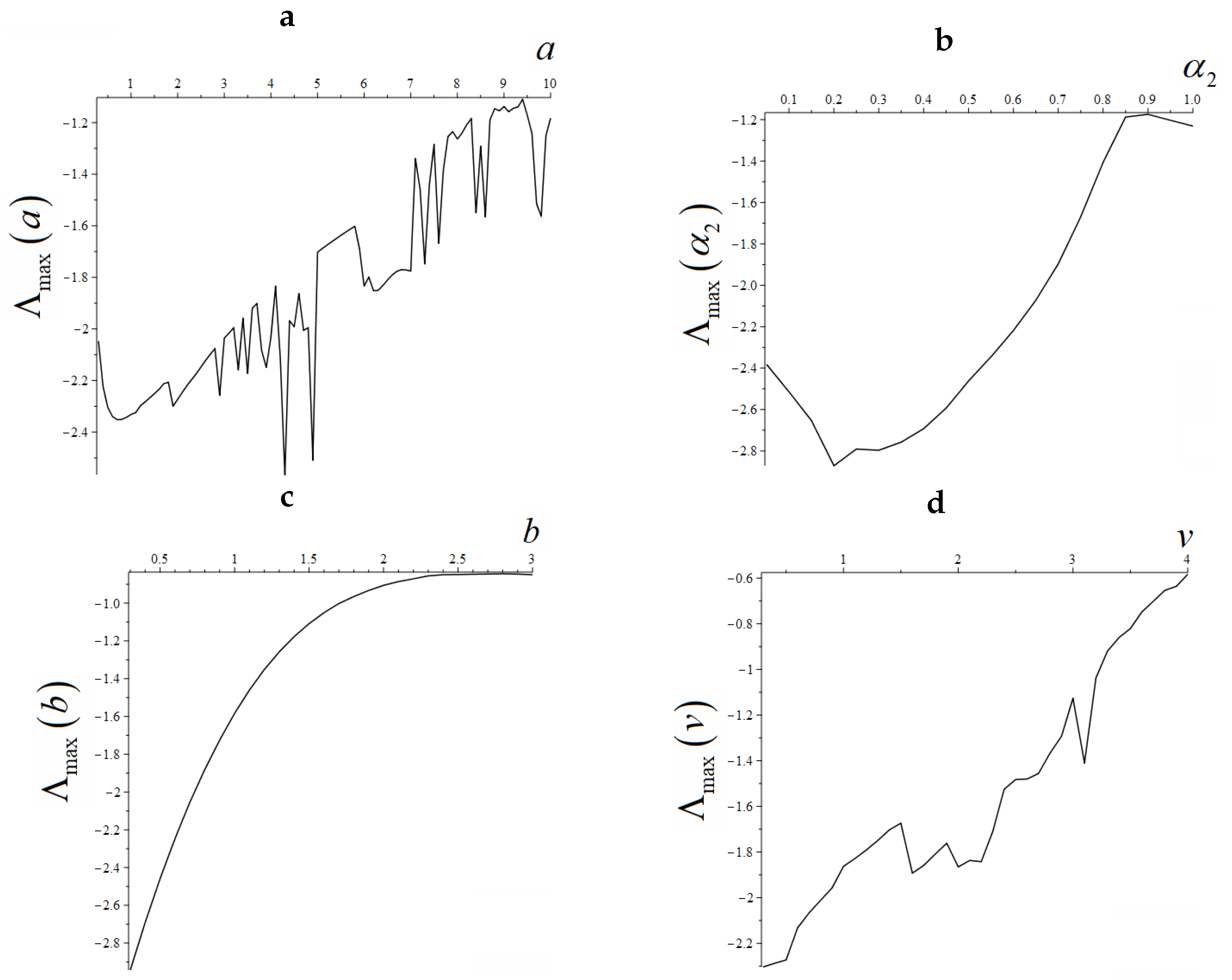
Example 5. 

Let us present other MLE spectra ${\mathsf{\Lambda }}_{max}\left({\alpha }_2\right)$, ${\mathsf{\Lambda }}_{max}\left(b\right)$, ${\mathsf{\Lambda }}_{max}\left(v\right)$ for the first MLE according to BWA for the FSDS system (4):

${\mathsf{\Lambda }}_{max}\left(a\right)$: $v=0.5,{\alpha }_1={\alpha }_2=b=1,t\in \left[0,100\right],x\left(0\right)=0.2,y\left(0\right)=0.3,$$a\in \left(0,10\right]$ with a step $\tau =0.1$.

${\mathsf{\Lambda }}_{max}\left({\alpha }_2\right)$: $v=0.5,a=0.1,{\alpha }_1=b=1,t\in \left[0,100\right],x\left(0\right)=0.2,y\left(0\right)=0.3,$${\alpha }_2\in \left(0,1\right]$ with a step $\tau =0.05$.

${\mathsf{\Lambda }}_{max}\left(b\right):v=0.5,a=0.1,b\in \left(0,3\right],{\alpha }_1={\alpha }_2=1,t\in \left[0,100\right],x\left(0\right)=0.2,y\left(0\right)=0.3$ c with a step $\tau =0.1$.

${\mathsf{\Lambda }}_{max}\left(v\right)$: $a=2,{\alpha }_1={\alpha }_2=b=1,t\in \left[0,100\right],x\left(0\right)=0.2,y\left(0\right)=0.3,$$v\in \left(0,4\right]$ with a step $\tau =0.1$.

Here we can see that all MLE spectra are negative, indicating that there are no chaotic modes for these examples (Figure 6).

8. Discussion

It should be noted that it is possible to refine the boundaries of bifurcation diagrams, for example, if we take into account the Householder procedure [33] in the BWA algorithm instead of the Gram–Schmidt orthogonalization, and also use more accurate numerical methods [19,20]. These studies, in my opinion, should explain the positive values in the spectrum of the maximum Lyapunov exponent, corresponding to chaotic regimes, and not to aperiodic regimes, as in Figure 5.

The question of the existence of chaotic regimes for FSDS remains open in this paper. However, a more detailed picture in the further study of the FSDS model can be obtained from maps of its dynamic regimes for various model parameters. Another direction of research may be related to the development of the FSDS model, which is related to the generalization of the Gerasimov–Caputo fractional order derivative (2) to the case of a variable fractional order [34]. Of interest is the study of FSDS in the case of arbitrary values of the parameter $\sigma$.

In the future, it is also planned to use experimental data on microseisms to refine the model parameters.

9. Conclusions

The article studies the Selkov fractional dynamical system, which is a mathematical model for describing microseisms, taking into account heredity. It is shown that the Selkov fractional dynamical system may have regular regimes. Numerical analysis shows that the regular regime is often characterized by a stable limit cycle on the phase plane, which determines the self-oscillatory regime. The presence of the Andronov–Hopf bifurcation, which arises in the classical Selkov dynamical system, is shown.

The MLE study showed that the spectra are mostly negative, indicating the absence of chaotic regimes. However, the MLE spectrum from the ${\alpha }_1$ parameter showed positive values, which, as was shown using criterion (12), do not correspond to chaotic regimes. Therefore, it is always necessary to check the results obtained by the BWA algorithm using various tests. This circumstance must be taken into account in further study of FSDS.