Article

DHGEEP: A Dynamic Heterogeneous Graph-Embedding Method for Evolutionary Prediction

1
College of Intelligence Science and Technology, National University of Defense Technology, Changsha 410073, China
2
College of Systems Engineering, National University of Defense Technology, Changsha 410073, China
*
Authors to whom correspondence should be addressed.
Mathematics 2022, 10(22), 4193; https://doi.org/10.3390/math10224193
Submission received: 12 October 2022 / Revised: 30 October 2022 / Accepted: 7 November 2022 / Published: 9 November 2022
(This article belongs to the Special Issue Complex Network Modeling: Theory and Applications)

Abstract

:
Current graph-embedding methods mainly focus on static homogeneous graphs, where the entity type is the same and the topology is fixed. However, in real networks, such as academic networks and shopping networks, there are typically various types of nodes and temporal interactions. The dynamical and heterogeneous components of graphs in general contain abundant information. Currently, most studies on dynamic graphs do not sufficiently consider the heterogeneity of the network in question, and hence the semantic information of the interactions between heterogeneous nodes is missing in the graph embeddings. On the other hand, the overall size of the network tends to accumulate over time, and its growth rate can reflect the ability of the entire network to generate interactions of heterogeneous nodes; therefore, we developed a graph dynamics model to model the evolution of graph dynamics. Moreover, the temporal properties of nodes regularly affect the generation of temporal interaction events with which they are connected. Thus, we developed a node dynamics model to model the evolution of node connectivity. In this paper, we propose DHGEEP, a dynamic heterogeneous graph-embedding method based on the Hawkes process, to predict the evolution of dynamic heterogeneous networks. The model considers the generation of temporal events as an effect of historical events, introduces the Hawkes process to simulate this evolution, and then captures semantic and structural information based on the meta-paths of temporal heterogeneous nodes. Finally, the graph-level dynamics of the network and the node-level dynamics of each node are integrated into the DHGEEP framework. The embeddings of the nodes are automatically obtained by minimizing the value of the loss function. Experiments were conducted on three downstream tasks, static link prediction, temporal event prediction for homogeneous nodes, and temporal event prediction for heterogeneous nodes, on three datasets. Experimental results show that DHGEEP achieves excellent performance in these tasks. In the most significant task, temporal event prediction of heterogeneous nodes, the values of precision@2 and recall@2 can reach 30.23% and 10.48% on the AMiner dataset, and reach 4.56% and 1.61% on the DBLP dataset, so that our method is more accurate at predicting future temporal events than the baseline.

1. Introduction

Complex networks provide an effective paradigm for studying the complexity and interactions of the real world, and have thus attracted considerable attention. Traditional mathematical methods have a limited ability to express the complex characteristics of large-scale networks, making it difficult to express many networks found in the real world [1]. In real-world scenarios, various aspects of the network change over time, including the structure, scale, and information contained in the network. Static networks cannot describe this general phenomenon, but the representation of dynamic networks reflects the dynamics of real-world situations [2]. However, most existing studies have focused on the static networks, and relatively little attention has been given to dynamic networks. Early researchers tried to use mathematical methods to study the evolution of dynamic graphs. Shang extended the static Estrada index to the dynamic setting [3], and based on this, Laplacian Estrada and normalized Laplacian Estrada indices of evolving graphs were proposed, and then he verified the indexes on the synthetic, randomly evolving small-world networks [4]. Unfortunately, this kind of approach requires manual extraction of the characteristics of dynamic networks. In recent years, graph-embedding techniques have been widely used for learning graph representations, allowing the structure and attribute information of a network to be input into a neural network formulation to obtain a low-dimensional representation vector. This has led to a significant improvement in network representation capabilities. These techniques have been applied to both static networks and dynamic networks. Dynamic network embedding is the current research hotspot [5], which can be divided into discrete and continuous approaches.
  • Discrete-Time Dynamic Graph
Generally, a discrete-time dynamic graph is generated by accumulating evolution across a window of consecutive timestamps to extract the desired information or apply static graph modeling techniques on the snapshots [6]. One idea is to improve the node embedding methods for static networks to adapt to the dynamic ones—for instance, incorporating random walks around dynamic networks into Bernoulli embeddings [7] and utilizing the novel dynamic personalized PageRank vectors based on the local network embedding on a static graph [8]. Another idea is to change the structure of a static graph neural network (GNN) to enable the structural and temporal features of discrete dynamic graphs to be automatically learned in a unified GNN framework. Many novel frameworks have been proposed, such as general temporal network-diffusion convolutional networks [9], an encoder–decoder architecture combined with long short-term memory (LSTM) [10], an automatic deep graph encoder [11], and an implicit hierarchical learning framework in hyperbolic space [12]. In addition, some researchers have introduced dynamic knowledge graphs as a perspective for studying dynamic graphs [13,14].
However, another difficult problem is whether it is appropriate to divide the time axis into equal lengths and perform aggregation to create a discrete time dynamic graph. It can be known that the density of events in the dynamic network is not evenly distributed over time. If the time division length is treated equally, the network size in some snapshots may be too large, whereas the network size in some snapshots will be too small, resulting in low correlation between snapshots and difficulties in mining dynamic network characteristics. Therefore, researchers have studied the method of dividing the time axis and the method of distinguishing the importance of snapshots. A temporal attention mechanism has been introduced [15], and a joint structural and temporal self-attention mechanism has been developed [16]. Based on the attention mechanism, Ma et al. proposed an adaptive graph convolution framework combined with an LSTM for feature extraction [17].
For different graphs and tasks, embedding different attributes of a dynamic graph will have different effects. Researchers have proposed algorithms to embed various characteristics of dynamic networks according to different research objects. Some have embedded the topology and evolutionary patterns of the dynamic network in a dynamic graph representation [18,19]. In addition, there are targeted methods to embed other features, such as the structural changes of the subgraph related to the target node [20], the long- and short-term dependencies, the spectrum of the Laplacian matrix of the graph structure at each snapshot [21], and the dynamic interests of users over a long period [22]. Graph-level features can usually indicate overall changes in structure and attributes. By embedding graph level features via multiple random walks, Beladev et al. jointly learned temporal graph-level representations and temporal node representations [23], and Hou et al. introduced an incremental learning paradigm and considered inactive subnetworks to better preserve the global topology at each time step [24].
Discrete dynamic networks “slice” continuous time into several discrete epochs, effectively mapping nodes and edges generated over a period of time to a sequence of snapshots. This paradigm is in line with people’s general understanding of dynamic graphs but ignores the dynamics in the snapshot, so it is difficult to realize the dynamic representation in the real sense, because the generation time of temporal edges in the discrete time dynamic graph is set to be the same as the timestamp of the graph snapshot, whereas in a real network, temporal edges can be generated at any time.
  • Continuous-time Dynamic Graph
Continuous dynamic graphs have been developed, which consist of a stream of dyadic events [25,26,27]. Continuous-time processing methods can be divided into time-coding-based methods and attention-mechanism-based methods. Researchers have studied time-coding technologies for inductive representation learning on dynamic graphs, such as learning a set of functions for learning communication and association between dynamic nodes [28]. Based on the functional time encoding proposed by Xu et al. [29], Xia et al. encoded continuous real-valued timestamps as vectors to preserve fine-grained time information [30], and Rossi et al. combined memory modules with graph-based operators to store long-term information [31]. Time-coding technology requires complex mathematical skills, and an attention mechanism is a lightweight and effective continuous-time processing method with strong scalability that can be combined with many other methods. Implementations include a temporal collaborative attention mechanism for jointly modeling collaborative signals and temporal effects [32], a selection mechanism with a dynamic message passing neural network [33], and a representation method of temporal knowledge graph with attention propagation using the temporal displacement between each event and the query timestamp [34].
Based on these two types of methods, researchers have attempted to mine and embed multiplex characteristics of dynamic graphs for enhanced representation learning. For identifying domain-specific laws within different temporal networks, Huang et al. captured the triad evolution process that preserves motif-aware high-order proximities [35], Liu et al. focused on predicting higher-order patterns in temporal hypergraphs [36], and Wang et al. encoded temporal network motifs via causal anonymous walks [37]. For future link prediction or dynamic graph recommendations, Du et al. exploited a graph-based neural Hawkes process for event propagation prediction with spatiotemporal characteristics [38], Yang et al. introduced meta-learning to extract hierarchical knowledge for few-shot dynamic link prediction [39], and Yang et at. incorporated temporal information and spatial information into neighbor embedding learning [40]. In addition, some researchers tried to learn graph representation from the perspective of the graph level and node level. Sun et al. generated stochastic representations to model the graph dynamics and uncertainties in hyperbolic space [41]. By considering the mutual evolution of micro- and macro-dynamics, Lu et al. captured the formation process and evolution pattern of a network [42]. Some researchers have modeled events at individual and collective scales and formulated them as event and node dynamics on a Hawkes process-based GNN [43]. In these studies, it can be seen that encoding different attributes of the temporal dynamic network can improve the performance of the model for different problems.
Continuous-time dynamic graphs are composed of streams of temporal events that can support continuous-time scenarios and thus be truly dynamic. However, most of the methods find it difficult to deal with the data structure of the event flow. Thus, most studies only generate the embedding for the final state of the dynamic graph, and it is difficult to inductively learn from a continuous-time dynamic graph. In addition, embed multiplex characteristics of dynamic graphs can enhance the performance of a method for different tasks.
  • Continuous-time Dynamic Heterogeneous Graph
One of the important characteristics of a real network is the heterogeneity of the nodes and their interactions. The heterogeneity of nodes represents entities having different functions, and the heterogeneity of edges represents different relationships. A dynamic heterogeneous graph not only expresses the changes in the topological complex structure of the graph and rich semantics, but also expresses the temporal evolution of the graph and various time preferences. This research is still in its infancy. Researchers have improved the heterogeneous network embedding method to adapt it to dynamic situations and improved the dynamic network embedding method to adapt it to heterogeneity. For example, Hu et al. introduced a relative temporal encoding strategy and node- and edge-type-dependent attention mechanisms for, respectively, handling dynamics and heterogeneity [44], Li et al. proposed a three-level attention mechanism to take network heterogeneity and dynamics into account at the same time [45], Xie et al. embedded an dynamic time-series into an online real-time-updated model [46], and Deng et al. used the heterogeneous fusion of multiple types of concurrent events for time-knowledge graph learning [47].
From the perspective of multivariate time series forecasting, researchers have studied dynamic, heterogeneous graph embedding by exploiting rich spatial relation information and temporal features [48] and converting event signals from dynamic heterogeneous graphs into event time series [49]. Furthermore, meta-paths are commonly used for dynamic heterogeneous graph representations. For example, Lu et al. captured the network structure and semantics by preserving the meta-path-based first- and second-order proximities [50], and Shi et al. considered the time dynamics in the evolution process to obtain the structure and semantics in a dynamic heterogeneous graph, with a meta-path method with an attention mechanism using the Hawkes process to model the evolution [51].
The research on dynamic heterogeneous graphs is still in its early stages, and there are many difficulties to be overcome. Firstly, the current dynamic graph model can only deal with one type of nodes and cannot model the temporal events between heterogeneous nodes. Secondly, the interactions between heterogeneous nodes often contain rich semantic information, so how to extract the semantic information contained in the temporal interactions of heterogeneous nodes is a key problem to be solved. Thirdly, from the perspective of temporal events, historical events have potential influences on the current node interactions, so it is necessary to consider that the impact of historical events on current interactions attenuates over time. Fourthly, from the perspective of the whole graph, the scale of the dynamic heterogeneous graph will accumulate over time, and the growth rate of the number of edges represents the trend change in the graph’s link generation, which is a continuous value with time. Thus, how to maintain the continuity of graph dynamics in dynamic, heterogeneous graph embedding is a problem that needs to be solved. Finally, from the perspective of nodes, node interactions at different times often show collective characteristics related to nodes at both ends. Therefore, when predicting the generation of future temporal events, the characteristics of nodes at both ends over time should be taken into account.
  • Our Work
In view of the above difficulties, we were inspired by a meta-path-based, dynamic heterogeneous graph-embedding method called THINE [51] and proposed DHGEEP (a Dynamic Heterogeneous Graph Embedding method for Evolutionary Prediction). DHGEEP mainly uses the Hawkes process to simulate the phenomenon that the influences of historical events will decay over time and introduces a temporal, heterogeneous meta-path and attention mechanism as the tool to extract semantic information and structural information to obtain dynamic, heterogeneous graph embedding. Inspired by the two methods for mining and embedding various characteristics of dynamic homogeneous graphs [42,43], we attempt to model the graph dynamics and the node dynamics. In [42], the micro-dynamics of the network consisted of events arranged chronologically, emphasizing the sequence of temporal events, while ignoring that the sequential events are the causes of the interaction between nodes, so it cannot model some emergencies in the network. Our method is more concerned with the relationship between the node’s own dynamics and the temporal events it produces and can learn the joint distribution between node dynamics and temporal events. In [43], TREND simulated the dynamics of nodes but did not model the graph dynamics, which cannot guarantee that the evolution scale of dynamic network is in line with the due characteristics. In addition, these two methods are only applicable to homogeneous dynamic networks. Thus, the most important contribution is the modeling of graph dynamics in the framework to represent the dynamics of the entire graph—that is, the scale of edges in the network accumulates over time, and the increasing speed of the scale represents the trend of the network’s ability to generate edges. In addition, the node dynamics are modeled in the framework, that is, the temporal edges generated on the same node show the law of distribution over time. Finally, we designed a loss function and update the parameters through the Adam optimizer.
The main contributions can be summarized as follows:
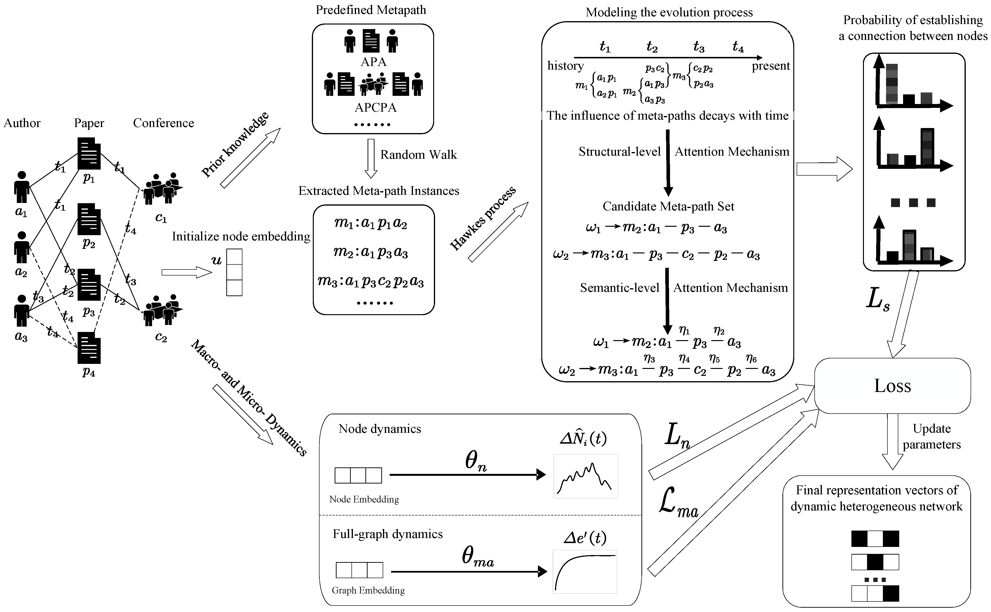
  • For the first time, we embed the dynamics of a whole graph into a dynamic heterogeneous network representation vector. In the past, the dynamic heterogeneous network-embedding methods have only focused on the semantic and time decay effects contained in the meta-path, while the dynamics of the whole network would affect the local embedding. As the so-called “collective influence individuals,” the traditional methods rarely modeled the evolutionary periodic effects from the overall perspective of the dynamic heterogeneous network. In this method, the current scale and trend of the whole graph are embedded into the representation vector so that the graph representation can represent the properties of the network from the perspective of the whole network.
  • For the first time, we embed node dynamics into the representation of the dynamic heterogeneous network. We have observed that in dynamic heterogeneous networks, although each event has its own individual characteristics, the temporal events generated on the associated nodes will be affected by the connectivity of shared heterogeneous nodes, and the connectivity of nodes changes with time, resulting in the similarity and collective characteristics between temporal edges changing with time. We define the collective characteristics of events at the same node as node dynamics. It provides a regularization mechanism that goes beyond a single event to ensure that the temporal edges on the node can conform to the joint distribution of node dynamics and time.
  • The experimental results on three real datasets show that DHGEEP is superior to several baselines.
The remainder of this paper is organized as follows. In Section 2, we formalize the problem. Section 3 describes the dynamic heterogeneous network embedding method proposed in this paper. Section 4 presents the experimental setup and results of the three downstream tasks. Section 5 summarizes the conclusions of this study.

2. Related Work

There has been relatively little research on prediction for heterogeneous dynamic networks, and so we have investigated 12 existing prediction strategies as baselines, which can be divided into two categories, shallow embedding models and deep embedding models. The shallow model is a machine learning model with few hidden layers. It first initializes the graph-embedding vector and then treats each element in the graph-embedding vector as a parameter to learn directly from the data. Compared with the shallow model, the deep model is a machine learning model with multiple hidden layers, which can better model the nonlinear relationship. The deep model is used to learn more complex features, and then the information is jointly encoded and fused to obtain the low-dimensional representation vectors of graphs. The first nine are shallow embedding models, and the last three are deep embedding models. The details of the methods are described below.
  • Deepwalk [52] and LINE [53]: Two static-homogeneous-network shallow-embedding methods based on the neighborhood information of nodes to obtain the representations, which were inspired by NLP problems.
  • Metapath2vec [54]: A static-heterogeneous-network shallow-embedding method based on the metapath to capture semantics and structure. The random swimming based on meta-path specifies the neighbor of a node and then uses a heterogeneous skip-gram model to implement embedding.
  • DySAT [16]: A dynamic-homogeneous-network shallow-embedding method. DySAT divides the dynamic network into different subgraphs of snapshots and then aggregates the information of each subgraph. It captures dynamics from two sources, structural neighborhood and temporary dynamics, and uses multiple heads of attention to capture multiple dynamics.
  • HTNE [55]: A dynamic-homogeneous-network shallow-embedding method based on the Hawkes process. HTNE integrates the Hawkes process into network embedding to discover the influence of historical neighbors on current neighbors.
  • MTNE [35]: A dynamic-homogeneous-network shallow-embedding method that simulates the evolution of networks. MTNE considers the effect of mesoscopic dynamics, especially the temporal dynamics of the particular motifs when the network evolves.
  • DHNE [56]: A dynamic-heterogeneous-network shallow-embedding method which constructs comprehensive historical-current networks based on subgraphs of snapshots in time step. Additionally, meta-paths are used to capture semantics.
  • StHNE [50]: A static-heterogeneous-network shallow-embedding method which can capture a network representation of the structure and semantics in the static heterogeneous map based on the first-order and second-order approximation of the meta-path.
  • DyHNE [50]: A dynamic-heterogeneous-network shallow-embedding method based on StHNE, which can learn the nodes’ embedding based on perturbation theory when the structure and semantics of the augmented adjacency matrix of the meta-path change.
  • MAGNN [57]: A static-heterogeneous-network deep-embedding method based on meta-path aggregation for static heterogeneous graphs.
  • HDGNN [58]: A dynamic-heterogeneous-network deep-embedding method which can integrate the characteristics of time evolution and capture the structural characteristics of attribute graphs and the dynamic complex relationships between nodes.
  • THINE [51]: A dynamic-heterogeneous-network deep-embedding method, which uses the Hawkes process to simulate the evolution of the temporal network and combines the attention mechanism and meta-paths.

3. Problem Formalization

In this section, we formalize the evolutionary model of dynamic heterogeneous networks. Consider a graph G = ( V , E , T , ϕ , φ ) , where V , E , and T represent the node set, edge set, and timestamp set, respectively. The heterogeneity of the network is reflected in the different types of nodes and edges, i.e.,  ϕ : V A , φ : E R , where A is the node-type set and R represents the edge-type set, | A | + | R | > 2 . The dynamics of the network are reflected in the nodes and edges at different time steps; i.e., edge e i j t E indicates that v i establishes a link relationship with node v j at t. Nodes may establish multiple relationships at different times, so there may be a large number of relationships between two nodes in the network.
In studying dynamic heterogeneous networks, the problem to be solved can be described as follows: for a dynamic heterogeneous network G = ( V , E , T , ϕ , φ ) , we must learn a mapping function f : V R d by comprehensively considering the temporal dynamics and heterogeneous structure information of the network, where d is the embedding dimension, d | V | . Finally, a low-dimensional vector of multi-type node embeddings is obtained.

4. Methods

In this section, we describe the details of the proposed dynamic heterogeneous graph-embedding method for evolutionary prediction (DHGEEP). The framework of DHGEEP is shown in Figure 1.
To combine the dynamic and heterogeneous information of the network, we adopt the same idea as many studies [35,55], and in a simple way, that is, using the negative Euclidean distance square for describing the contributions of two nodes v i , v j V to the establishment of an edge between the two as
β x , y = | u x u y | 2
where β x , y is the influence of the node pair, and  u x and u y represent the embedding vectors of nodes v x and v y . Based on this assumption, we decided to use temporal meta-paths to obtain the mutual influences between various types of nodes. The meta-path-based approach has been proven to be effective in dynamic heterogeneous networks [50,51]. Similarly to decomposition and autoencoder-based approaches, one of the major advantages of the encoders based on random walks is that they provide an embedding function without needing to be combined with a decoder [2]. The meta-path M is defined as a 1 r 1 a 2 r 2 a 3 r 3 r l 1 a l , where r i R represents the node type and a i A represents the edge type. Obviously, a meta-path is a complex relationship; for example, an instance m of M consists of a node sequence ( v 1 , v 2 , , v l ) , which describes the semantic information contained from v 1 to v l . In our method, we define meta-paths with specific information and structures in heterogeneous networks to capture node embeddings. Taking academic networks as an example, we pick five well-established meta-paths to capture the network information. For example, for two authors collaborating on a paper, we adopt the author–paper–author meta-path, whereas two authors publishing papers at the same conference is represented by the meta-path author–paper–conference–paper–author. We define candidate meta-paths S ( t ) for temporal edge e i j t E . This refers to a meta-path set that contains all temporal edges generated before time t that involve source node v i and all temporal edges in the meta-path instance m. The embedding of a node is determined by the candidate meta-path and the properties of the node itself.
However, not all meta-paths in the entire time period have the same impact on the node embedding representation at the current moment. Obviously, a shorter time period means that an event has a greater impact on the node embedding, so we consider the Hawkes process to model the impact of historical events on the current node representation vector. Typically, the earlier an event occurs, the less of an impact it has on the present time. We apply the Hawkes process to each node, with  η s , η m , and η e denoting the effect of candidate meta-path sets, meta-path instances, and timing edges. Note that for t m < t , the impact of a candidate meta-path set is given by
η s ( t ) = t m < t η m ( t )
Specifically, in a dynamic heterogeneous network, every meta-path contains its own semantics, and for different downstream tasks, different meta-paths have slightly different roles. Thus, we use an attention mechanism to capture differences in the semantics contained in the meta-path. Formally, the weights of different types of meta-paths are defined as
ω b = e ω b c e ω c
where the meta-paths pre-defined by prior knowledge are represented by c and ω b represents the weight of meta-path b. Thus, Equation (1) becomes
η s ( t ) = t m < t ω M × η m ( t )
where ω M represents the weight of M. Similarly to Equation (1), the effect of a meta-path instance η m ( t ) is the synthesis of the effect of all temporal edges e i j t that make up meta-path instance m. Therefore, we write
η m ( t ) = e i j t m η e i , j t ( t )
Specifically, e i j t indicates that nodes v i and v j generate a connection at time t i , j , so edge e i j t can be represented by the current nodes at both ends, i.e.,  v i and v j . Similarly to Equation (2), the different numbers of hops to the target edge mean that each edge has a different effect. Therefore, we use another attention mechanism for structurally differentiated influences, and calculate the edge weights as
θ h o q = e θ h o q z e θ h
where h o q represents the number of hops from edge e o q to the source node, and the weight of hop h o q is θ h o q . We use z to represent the number of candidate edges, and  z increases with z. That is, the effect of a meta-path instance can be redefined as
η m ( t ) = θ h i j × e i j m η e i , j ( t )
We must also consider the influence of the Hawkes process, that is, the attenuation effect of historical events. Therefore, the influence of the final timing edge can be expressed as
η e i j ( t ) = η i , j × t i , j < t κ t t i , j
where κ t t i , j represents the time decay effect; generally, an exponential function is used, and here we use e δ i t t i , j , where δ is a trainable node-related parameter used to adjust the scale of the temporal decay effect. The impacts of previous events decrease with time, so the influences of events over a certain age on the present can be ignored. To reduce the computational complexity, we select the n meta-path instances generated at time t. However, the level of influence η m ( t ) at which these meta-path instances can be omitted is difficult to determine, so we use n as a hyperparameter for learning. Similarly, for each meta-path instance m, we only need to select some candidate edges closest to the selected node for training. Considering that the impact of the edges η e i j ( t ) is also difficult to estimate, the number of candidate edges z is used as a hyperparameter.
Through the above methods, we model the edges in dynamic heterogeneous networks and obtain multi-type node embeddings including semantic information, structural information, and temporal dynamic information. The ability to generate temporal edges between any pair of nodes v x and v y at t is then calculated as the following conditional strength function:
λ ˜ x , y ( t ) = η x , y + η s ( t ) = η x , y + t m < t ( ω M × e i j m θ h i j × η e i j ( t ) )
where λ ˜ x , y ( t ) is the conditional strength function representing the possibility of a connection between nodes v x and v y at time t. We transform this to λ x , y ( t ) = e x p ( λ ˜ x , y ( t ) ) , so that λ x , y ( t ) takes values from 0 to 1.

4.1. Modeling the Dynamics of Nodes

In the study of dynamic networks, the events represented by each temporal edge show strong individual characteristics, but do not occur in isolation and often have correlations that are reflected in multiple events. Regarding the connections of common nodes at both ends, different nodes exhibit different trends, and individual nodes may also produce different trends in different periods. In real networks, the events related to the network are the edges generated by the nodes. For example, in a social network, user1 and user2 have different degrees of activity at time t 0 ; specifically, user1 has a narrower social profile, and user2 is more socially adept. At some later time t 1 , user2 becomes more active (possibly because he has more followers). Thus, each node’s event set matches its own arrival rate, which is a time-varying property of the node itself, which we call the node dynamics. Unlike event dynamics for the individual characteristics of an event, the node dynamics are used to model the event’s collective characteristics at a node at different periods. In other words, the node dynamics provide a mechanism for the generation of defined collective events. Specifically, the node dynamics of a node at time t can be calculated by the number of new events occurring at that node at t, denoted as Δ N i ( t ) . We introduce the following estimator with fully connected layers for the node dynamics:
Δ N ^ i ( t ) = FCL n ( h i t ; θ n )
where the input is the time representation h i t and the output Δ N ^ i ( t ) is the new event that occurs at node i at time t. The number of predictions θ n contains the parameters of FCL n .

4.2. Modeling the Dynamics of the Entire Graph

In this section, we describe how to model the dynamics of the whole graph. The dynamics of the whole graph reflect the overall scale of the network changes with time from a macro perspective. Here, the scale refers to the number of active nodes or active edges in the network, which usually exhibits an obvious change distribution, such as an S-shaped sigmoid curve or power-law form. This phenomenon describes the periodicity that is common in real-world networks: from increasing to decreasing, or from small to huge. The changes in network scale at each time follow a certain trend, and the change law provided by this trend describes overall evolution information and structural information. Modeling the whole graph’s dynamics allows us to improve the representation ability of dynamic heterogeneous networks.
The dynamics of the whole graph represent the evolutionary process at the network scale. The appearance (or disappearance) of nodes will inevitably result in the generation (or deletion) of edges. Here, we focus on the changes in scale of the edges. Let G = ( V , E , T ) be a dynamic network, and let the full-graph dynamics be expressed as A = { e ( t ) } t = t 1 | T | , where e ( t ) represents the number of edges generated by all nodes up to time t. We use n ( t ) to represent the number of nodes at time t. Each node i connects to some other node j at time t with a connection rate of r ( t ) .
In addition, we assume that the average number of reachable neighbors of node i can be expressed as ι t . Therefore, we define the dynamics of the whole graph as
Δ e ( t ) = n ( t ) r ( t ) ι t
where n ( t ) is the number of nodes added to the network at time t, the value of which can be obtained. Here, we make an assumption about the expression of ι t . Considering the dense power law in network evolution, the average number of reachable neighbors of node i can be obtained as ι t = ζ n t 1 γ , where ζ represents the linear sparse coefficient and γ represents the power-law coefficient exponent. Thus, at the next moment, each node attempts to connect with another ζ ( n ( t ) 1 ) γ nodes at a connection rate of r t , where ζ and γ are hyperparameters to be learned.
We also modeled the connection rate r ( T ) , which is related to the timing information and structural information of the network. As the initial edges disappear with the evolution of the network, the connection rate should be a decreasing function of time. The structural changes of the network also affect the connection rate and play a significant role in the dynamics of the whole graph. The connection rate can be written as
r ( t ) = 1 | E | ( i , j , t ) E σ u i u j 2 2 t θ
where θ represents the temporal index and σ ( x ) is a sigmoid function. The numerator models the maximum connection rate of the network, which decays over time.

4.3. Design of the Loss Function

In this section, we design a novel comprehensive loss function to update the parameters of the model. At time t, the probability that nodes v x and v y produce a connecting edge is
p v x , v y S ( t ) = λ x , y ( t ) y λ x , y ( t )
where S ( t ) represents the set of candidate meta-paths before time t and y = V \ v x . Due to the exp(·) transfer function introduced in the Equation (9), p v x , v y S ( t ) is actually a softmax unit applied to λ ˜ x , y t , which can be optimized approximately via negative sampling [59]. Obviously, to calculate the above formula, we need to the node information throughout the network, so we apply the negative sampling technique to reduce the computational cost [55]. We collect K negative samples according to P n ( v ) , which is positively related to d v 3 / 4 , where d v represents the degree of node v. The probability of establishing a connection between all node pairs can be written as
log L = ( v x , v x ) E log p ( v x , v y S ( t ) )
We define the semantic loss L s as
L s = log σ λ ˜ x , y ( t ) k = 1 K E v k P n ( v ) log σ λ ˜ x , k ( t )
where the sigmoid function σ ( x ) = 1 1 + e x . The generation of events should be consistent with the evolution of the node dynamics, so the loss of node dynamics must be defined in such a way that Δ N i ( t ) accurately estimates the probability of node occurrence at the current moment, Δ N ^ i ( t ) . In real scenarios, nodes with great quantities of new links may suddenly appear at some time. For example, many users may buy a new product immediately after it is launched. To prevent our model from focusing on these nodes, we employ the following combination of smoothed L 1 and L 2 losses [60]:
L n ( i , t ) = 0.5 ( Δ N ^ i ( t ) Δ N i ( t ) ) 2 , | Δ N ^ i ( t ) Δ N i ( t ) | < 1 | Δ N ^ i ( t ) Δ N i ( t ) | 0.5 . otherwise
When the input is large, the loss function is less sensitive to outliers, and when the input is small, the oscillation of the loss function is relatively small.
We also need to consider the constraints of the full-graph dynamics. In a dynamic heterogeneous network, the alignment of the amount of edges is expressed as A = { e ( t ) } t = t 1 | T | , and the change in the number of sides is expressed as Δ e t 1 , Δ e t 2 , Δ e t 3 , , where Δ e t i = e t i + 1 e t i . These parameters are learned by minimizing the following expression:
L m a = t T Δ e ( t ) Δ e ( t ) 2
Finally, we obtain the total loss function L in the form
L = L s + ϵ L n ( i , t ) + τ L m a
where ϵ and τ are predefined scaling factors. In our algorithm, the graph representation vector is initialized at the beginning. In the training, the graph representation vector and model parameters are updated using the Adam method to minimize the loss function. DHGEEP implements the propagation of deep information over shallow models, so there is no explicit formula to calculate the representation vector of the dynamic heterogeneous network, but the representation vector is learned together with the model to finally obtain a satisfactory graph representation. The algorithmic details of DEGEEP are shown in Algorithm 1 below.
Algorithm 1 DEGEEP: Algorithm for dynamic heterogeneous network embedding.
1:
Input: dynamic heterogeneous network G = ( V , E , T , ϕ , φ ) ; the meta-path set M, epoch.
2:
Output: Optimized model parameters θ ; the node represents the vector u.
3:
Initialize the node representation vectors u.
4:
Initialize the parameters to be learned θ .
5:
Initialize the Iterations = 0.
6:
While Iterations ≤ epoch do :
7:
   By using random walk, all sequential meta-path instances before time t are extracted
8:
    from G according to the defined set of meta-path M.
9:
     for each node in V do:
10:
      Extract the most recently generated s edges on the node
11:
       for each edge do:
12:
         The candidate meta-paths S ( t ) are obtained according to the sampling strategy
13:
            for each metapath instance m of S ( t ) do:
14:
                 for each edge of m do:
15:
                 Using Hawkes process, as Equation (8) to calculate the influence of each edge
16:
                 end for
17:
                Using attention mechanism to calculate the influence of the meta-path
18:
                instance m as Equations (5)–(7)
19:
            end for
20:
           Using attention mechanism to get the influence of the meta-path instance m
21:
           Calculate the influence of candidate meta-path set S ( t ) according to Equations (2)–(4)
22:
          end for
23:
    end for
24:
   The intensity of temporal edges between nodes is calculated as Equation (9)
25:
   the semantic loss L s is calculated as Equations (13)–(15)
26:
   % Macro and micro constraints
27:
    for node in V do:
28:
         The dynamic estimator of the node is calculated as Equation (10)
29:
    end for
30:
   Calculate the loss at the node level as Equation (16)
31:
    for every time in G do:
32:
         Calculating the dynamic estimator of the whole graph as Equations (11) and (12)
33:
    end For
34:
   Calculate the loss on the change trend of the whole map as Equation (17)
35:
   Calculate the loss value as Equation (18)
36:
  Based on Adam to minimize losses, the parameters is optimized and the node represents u is updated
37:
    Iterations = Iterations + 1
38:
End While

5. Experiments

5.1. Datasets

We investigated three datasets: AMiner, DBLP, and Yelp. The three datasets are described below:
  • AMiner: This dataset contains data on papers published in top-level journals and presented at conferences in the computer science field. The data are provided by the scientific and technological information and mining platform of Tsinghua University and include author, paper, and venue nodes from research fields such as data mining, medical information, theory, visualization, and databases. There are two types of temporal heterogeneous events, cooperative relationships (A-A) and submission relationships (A-V). The temporal link prediction task aims to predict temporal events in the latest period of time.
  • DBLP: This dataset contains data relating to top-level conference papers in the computer field, including author, paper, conference, and other nodes. Events include cooperation (A-A) and participation (A-V) and subsequent events involving databases, data mining, information retrieval, artificial intelligence, and others. The tasks are the same as for AMiner.
  • Yelp: This dataset consists of comments between users and merchants published by the Yelp comment platform. The network consists of user, business, and star nodes; and there are three types of sequential events. The link prediction task involves predicting the temporal events in the latest period of time.
Details of the datasets are presented in Table 1.

5.2. Offline Training

All experiments were performed on a dual-core computer with 128 GB RAM and an 11 GB NVIDIA GeForce RTX 2080ti GPU, with an Intel(R) Xeon(R) Platinum 8260 L CPU @ 2.40 GHz and CUDA version 11.0. The model was written in Pytorch 1.7.0. The following describes the parameter settings in the experiment. The Adam optimizer’s learning rate was set to 0.001, the batch size was set to 1000, the epoch number was set to 100, the embedded dimensions numbered 100, the number of walks of each node was set to 15, the walk length was 30, the number of candidate meta-path instances was n = 25 , the number of candidate edges was 6 ( z = 6 ), and the number of negative samples was 6. The baseline algorithms were introduced in the related work, and in the experiment, we changed the form of dynamic heterogeneous graph data to adapt to the application scope of the baseline algorithms. The results for the baseline methods were obtained from [51].

5.3. Results and Analysis

First, we applied DHGEEP for training and output of the current graph representation vector afterward, and then embedded the resulting graph into the downstream task. We verified the advantages of the proposed method through three experiments, one based on a static task and two based on dynamic tasks. The static task involved link prediction, which tests the capability of the graph-embedding method to capture structural information. The two dynamic tasks were homogeneous-temporal-event prediction and heterogeneous-temporal-event prediction, which examine the ability of graph-embedding methods to capture network dynamics.
1
In the link prediction task, according to Equation (1), the embedding vector of the edge is represented by the embedding vector of the two nodes, namely, e x , y = u x u y . In this task, a link prediction task can be regarded as a classification task. The test data consist of positive and negative links. Positive links are the actual links present in the future subgraph or test graph. Additionally, a test graph is split chronologically from the training graph to evaluate the model’s performance. Therefore, edges in this test graph or subgraph are considered positive examples. From the sample test graph, an equal number of non–edge node pairs are sampled as negative links. Based on these settings, we used a logistic regression classifier for the link prediction task with input e x , y . In the logical regression classifier, we established a regression formula for the classification boundary according to the sampling results. A common gradient boosting method was used in the process of fitting parameters. After training, we found the best regression coefficient for classification. For the Yelp dataset, the link prediction task is to predict the co-user relationships regarding goods, that is, whether two users have purchased and used the same goods. As for the two academic networks, AMiner and DBLP, the prediction task is to predict the relationship between authors, that is, the co-author relationship. The datasets do not contain the co-author edges; that is, there are no edges between authors. During training, 25% of author–paper (AP) edges were randomly deleted, because the meta-path author–paper–author (APA) implies co-author information, and there may be problems with information leakage. For Yelp, the connections between users were determined by whether they were friends in the original dataset. Similarly, we removed 25% of user–business (UB) edges and then trained a logistic regression classifier to predict the connections between users. In each dataset, we randomly selected 25,000 edges as positive edges and 25,000 as negative edges. In this task, we selected three common indicators of static network link prediction, AUC, f1, and acc. The link prediction results are listed in Table 2.
In Table 2, we can see that the methods using time information (DySAT, HTNE, MTNE, DHNE, DyHNE, HDGNN, THINE, and DHGEEP) are obviously better than the static-graph methods (Deepwalk, LINE, Metapath2vec, StHNE, and MAGNN), which further illustrates the importance of time information. As for network heterogeneity, the method considering network heterogeneity is not better than the method based on a homogeneous network, which shows that the influence of network heterogeneity is not as great as that of network dynamics in this task.
2
In the task of predicting temporal events of homogeneous nodes, we predicted the connections generated by the nodes of the same type. Taking the academic networks as an example, we predicted the future cooperative relationship between authors, that is, the co-author relationship. For the relationships contained in some specific meta-paths, such as APA, we selected the first 80% of all instances in the dataset, recorded these as time t, and used the events before this as the training set. The remaining data were used as the test set. In the experiment, the node embeddings obtained by various methods were used as input, and the negative square Euclidean distance was used to estimate the probability of generating edges between nodes to predict the connecting edge with the highest probability of generating nodes after t. We only conducted this experiment on the two academic datasets. Finally, we evaluated the performances of the various algorithms. In this task, predicting temporal events of homogeneous nodes is seen as a ranking problem. For every test node, its most probable future neighbors are ranked and compared with actual future neighbors. With our settings, the top K possible edges are ranked in a test graph and compared with the ground truth edges. Finally, the metrics chosen for this ranking problem were precision@K and recall@K. For the task of predicting temporal events of homogeneous nodes, we set K = 5 or K = 10 . The experimental results are presented in Table 3. Some of the baseline methods are only suitable for homogeneous networks and therefore cannot accurately represent the characteristics of dynamic heterogeneous networks. In addition, for the Yelp dataset, the differences are too large among the numbers of nodes of the three types. For example, there are 24,586 user nodes and only 5 star nodes. Thus, there are too few predictable results for predicting temporal events, so this dataset was not used in the experiment.
It can be seen from the experimental results in Table 3 that our DHGEEP method is effective at predicting temporal events at homogeneous nodes. Additionally, we can see that the methods considering time information (DySAT, HTNE, MTNE, DHNE, DyHNE, HDGNN, THINE and DHGEEP) are better than those with static graphs (Deepwalk, LINE, Metapath2vec, StHNE, and MAGNN). On average, this advantage is not as obvious as that in the last task. In addition, we can see that the deep methods (MAGNN, HDGNN, THINE, and DHGEEP) are generally superior to the shallow methods (Deepwalk, LINE, DySAT, HTNE, MTNE, Metapath2vec, StHNE, DHNE, and DyHNE). This means that the deep models can obtain more comprehensive information than the shallow models.
3
In order to prove that DHGEEP can well handle the heterogeneity of the network, we applied DHGEEP to the temporal event prediction of heterogeneous nodes in addition to the temporal event prediction of homogeneous nodes. This task was essentially the same as Task 2, except that the objects for predicting temporal events were different. As in the above task, the metrics chosen in this ranking problem were precision@K and recall@K. In the task of predicting temporal events of heterogeneous nodes, we set K = 2 or K = 4 . Specifically, we predicted the connections generated by different types of nodes. Taking the academic networks as an example, we predicted an author’s future participation in a conference, that is, the A–C relationship. The training process and testing methods were the same as those in Experiment 2. We only conducted this experiment using the two academic datasets. The experimental results are presented in Table 4. Our method achieved the highest precision and recall, which shows that DHGEEP can well handle the heterogeneity of the dynamic network. The pattern shown in Table 4 for the AMiner dataset is less obvious than that for the DBLP dataset. We could still find a pattern similar to that shown in the above tasks. The methods considering time information (DySAT, HTNE, MTNE, DHNE, HDGNN, THINE and DHGEEP) are better than the methods using static graphs (Deepwalk, LINE, Metapath2vec, and MAGNN). In addition, the deep methods (MAGNN, HDGNN, THINE and DHGEEP) are generally superior to the shallow methods (Deepwalk, LINE, DySAT, HTNE, MTNE, Metapath2vec, and DHNE). This means that the deep models can obtain more comprehensive information than the shallow models.
In this section, we introduced the results and analysis of the experiment. The experimental results showed that DHGEEP can perform well on three tasks with three datasets, which proves that DHGEEP can effectively capture the information of dynamic heterogeneous networks. In addition, we also found that the graph-embedding methods considering the dynamics are often better than the methods using static graphs, and the deep models are often better than the shallow models. Unfortunately, our comparison with other methods did not involve statistical tests but only compared the results. Therefore, we will try to carry out this part of the work in the future.

6. Conclusions

In this paper, we considered the influence of graph heterogeneity on dynamic graph evolution and proposed a temporal event prediction method of dynamic heterogeneous networks, DHGEEP (a dynamic heterogeneous graph embedding method for evolutionary prediction). Firstly, DHGEEP assumes that the generation of each temporal edge is caused by historical events, so it uses the Hawkes process to simulate the influences of historical temporal events on the present. Then, the temporal meta-paths and two-level attention mechanism are used to capture different structural information and semantic information. Finally, by integrating graph dynamics and node dynamics in the graph embedding framework, the macro evolution of dynamic network and the changes in node connectivity capability over time are simulated, which influences the generation of future temporal event prediction from the trend of network scale evolution at the graph level and the trend of timing events at the node level. Experiments were carried out on three downstream tasks of static link prediction, homogeneous-temporal-event prediction, and heterogeneous-temporal-event prediction on three datasets. The experimental results show that DHGEEP achieved good performance in the three tasks. In the static link prediction task, the value of AUC reached 91.57% on the AMiner dataset, 94.72% on the DBLP dataset, and 79.99% on the Yelp dataset. In the homogeneous-temporal-event prediction task, the values of precision@5 and recall@5 reached 14.59% and 4.81% on AMiner, and 11.94% and 3.67% on DBLP. In the heterogeneous homogeneous-temporal-event prediction task, the values of precision@2 and recall@2 reached 30.23% and 10.48% on the AMiner dataset, and reached 4.56% and 1.61% on the DBLP dataset.
Although our method achieved good results in these experiments, some issues remain. Firstly, our method is essentially transductive, as it relies on predefined meta-paths to obtain node embedding. However, in some scenarios, the prior knowledge may not be available. Therefore, in future work, we expect to develop a scalable inductive method which will not use the temporal meta-paths but other technologies, such as a graph neural network, to ensure that it can be used in scenarios without prior knowledge and allows transfer of knowledge to unseen graphs. Secondly, DHGEEP can only predict whether the timing edge will exist in the future, and cannot predict when the timing edge will occur. Recently, Rakshit et al. introduced the novel task of predicting the time of the link in consideration [28], which has great potential for applications in recommendation systems. Therefore, in future work, we expect to obtain a dynamic heterogeneous graph-embedding framework that will jointly learn whether and when future links will be generated, that is, the joint distribution of temporal and structural properties, to automatically predict the existence of future temporal events and the occurrence time of temporal events. Using such a method to understand which items a user will buy at a particular time will lead to better recommendations and higher efficiency. Thirdly, the edges in the network often exhibit complex connections. Recently, it has been found that designing high-order patterns of multiple node interactions is important for determining the evolution laws of dynamic networks [36]. Therefore, in future work, we will consider the high-order interaction patterns in the network to predict the full-spectrum high-order patterns in dynamic heterogeneous hypergraphs. Fourthly, the continuous-time dynamic heterogeneous networks we studied are defined based on the dynamics and heterogeneity of nodes and edges, which are different from the discrete-time dynamic networks in terms of model and data structure. However, what is interesting is that if we study dynamic heterogeneous networks from the perspective of dynamic evolution rather than from the perspective of nodes and edges in the network, the concepts of continuity and discreteness are not completely separated. For example, in a hybrid multi-agent system, continuous-time and discrete-time agents concurrently exist and communicate through local interaction. Based on this, Shang et al. studied resilient group consensus in heterogeneously robust networks with hybrid dynamics, which broke through the barrier between continuous-time dynamic heterogeneous networks and discrete-time dynamic heterogeneous networks [61]. Therefore, in future work, we plan to study the representation of dynamic heterogeneous networks with hybrid dynamics.

Author Contributions

All authors contributed to the study conception and design. Material preparation, data collection, and analysis were performed by L.C., C.Z. and H.L. The first draft of the manuscript was written by L.C. and checked by L.W. and J.C. All authors commented on previous versions of the manuscript. All authors read and approved the final manuscript.

Funding

This work is funded by National Natural Science Foundation (NNSF) of China under grant 62173336; the Scientific Research Plan of National University of Defense Technology under grant number ZK-20-38; the Postgraduate Research and Innovation Project of Hunan Province under grant CX20210085.

Institutional Review Board Statement

Not applicable.

Informed Consent Statement

Not applicable.

Data Availability Statement

Data can be obtained through the following link: https://dblp.org, https://www.yelp.com/dataset, https://www.aminer.cn/data/ (accessed on 11 October 2022).

Conflicts of Interest

The authors declare no conflict of interest.

References

  1. Porter, M.A. Nonlinearity + Networks: A 2020 Vision. In Emerging Frontiers in Nonlinear Science; Kevrekidis, P.G., Cuevas-Maraver, J., Saxena, A., Eds.; Springer International Publishing: Cham, Switzerland, 2020; pp. 131–159. [Google Scholar] [CrossRef]
  2. Kazemi, S.M.; Goel, R.; Jain, K.; Kobyzev, I.; Sethi, A.; Forsyth, P.; Poupart, P. Representation Learning for Dynamic Graphs: A Survey. J. Mach. Learn. Res. 2020, 21, 2648–2720. [Google Scholar]
  3. Shang, Y. The Estrada index of evolving graphs. Appl. Math. Comput. 2015, 250, 415–423. [Google Scholar] [CrossRef]
  4. Shang, Y. Laplacian Estrada and normalized Laplacian Estrada indices of evolving graphs. PLoS ONE 2015, 10, e0123426. [Google Scholar] [CrossRef] [PubMed]
  5. Barros, C.D.T.; Mendonça, M.R.F.; Vieira, A.B.; Ziviani, A. A Survey on Embedding Dynamic Graphs. ACM Comput. Surv. 2021, 55, 1–37. [Google Scholar] [CrossRef]
  6. Jin, D.; Kim, S. On Generalizing Static Node Embedding to Dynamic Settings: A Practitioner’s Guide. In Proceedings of the Fifteenth ACM International Conference on Web Search and Data Mining, Tempe, AZ, USA, 21–25 February 2022; pp. 410–420. [Google Scholar] [CrossRef]
  7. Chen, C.; Tao, Y.; Lin, H. Dynamic Network Embeddings for Network Evolution Analysis. arXiv 2019, arXiv:1906.09860. [Google Scholar]
  8. Guo, X.; Zhou, B.; Skiena, S. Subset Node Representation Learning over Large Dynamic Graphs. In Proceedings of the 27th ACM SIGKDD Conference on Knowledge Discovery & Data Mining, Singapore, 14–18 August 2021; Association for Computing Machinery: New York, NY, USA, 2021; pp. 516–526. [Google Scholar] [CrossRef]
  9. Wang, Y.; Li, P.; Bai, C.; Leskovec, J. TEDIC: Neural Modeling of Behavioral Patterns in Dynamic Social Interaction Networks. In Proceedings of the Web Conference, Ljubljana, Slovenia, 25–29 April 2021; pp. 693–705. [Google Scholar] [CrossRef]
  10. Chen, J.; Zhang, J.; Xu, X.; Fu, C.; Zhang, D.; Zhang, Q.; Xuan, Q. E-LSTM-D: A Deep Learning Framework for Dynamic Network Link Prediction. IEEE Trans. Syst. Man Cybern. Syst. 2021, 51, 3699–3712. [Google Scholar] [CrossRef] [Green Version]
  11. Goyal, P.; Kamra, N.; He, X.; Liu, Y. DynGEM: Deep Embedding Method for Dynamic Graphs. arXiv 2018, arXiv:1805.11273. [Google Scholar]
  12. Yang, M.; Zhou, M.; Kalander, M.; Huang, Z.; King, I. Discrete-Time Temporal Network Embedding via Implicit Hierarchical Learning in Hyperbolic Space. In Proceedings of the 27th ACM SIGKDD Conference on Knowledge Discovery & Data Mining, Singapore, 14–18 August 2021; Association for Computing Machinery: New York, NY, USA, 2021; pp. 1975–1985. [Google Scholar] [CrossRef]
  13. Li, Z.; Jin, X.; Li, W.; Guan, S.; Guo, J.; Shen, H.; Wang, Y.; Cheng, X. Temporal Knowledge Graph Reasoning Based on Evolutional Representation Learning. In Proceedings of the 44th International ACM SIGIR Conference on Research and Development in Information Retrieval, Montréal, BC, Canada, 11–15 July 2021; Association for Computing Machinery: New York, NY, USA, 2021; pp. 408–417. [Google Scholar] [CrossRef]
  14. Wu, J.; Cao, M.; Cheung, J.C.K.; Hamilton, W.L. TeMP: Temporal Message Passing for Temporal Knowledge Graph Completion. In Proceedings of the 2020 Conference on Empirical Methods in Natural Language Processing (EMNLP), Online, 16–20 November 2020; pp. 5730–5746. [Google Scholar] [CrossRef]
  15. Fathy, A.; Li, K. TemporalGAT: Attention-Based Dynamic Graph Representation Learning. In Advances in Knowledge Discovery and Data Mining; Lecture Notes in Computer Science; Lauw, H.W., Wong, R.C.W., Ntoulas, A., Lim, E.P., Ng, S.K., Pan, S.J., Eds.; Springer International Publishing: Cham, Switzerland, 2020; Volume 12084, pp. 413–423. [Google Scholar] [CrossRef]
  16. Sankar, A.; Wu, Y.; Gou, L.; Zhang, W.; Yang, H. DySAT: Deep Neural Representation Learning on Dynamic Graphs via Self-Attention Networks. In Proceedings of the 13th International Conference on Web Search and Data Mining, Houston, TX, USA, 22 January 2020; pp. 519–527. [Google Scholar] [CrossRef] [Green Version]
  17. Huang, R.; Ma, L.; He, J.; Chu, X. T-GAN: A deep learning framework for prediction of temporal complex networks with adaptive graph convolution and attention mechanism. Displays 2021, 68, 102023. [Google Scholar] [CrossRef]
  18. Lei, K.; Qin, M.; Bai, B.; Zhang, G.; Yang, M. GCN-GAN: A Non-Linear Temporal Link Prediction Model for Weighted Dynamic Networks. In Proceedings of the IEEE INFOCOM 2019—IEEE Conference on Computer Communications, Paris, France, 29 April–2 May 2019; pp. 388–396. [Google Scholar] [CrossRef] [Green Version]
  19. Wang, J.; Jin, Y.; Song, G.; Ma, X. EPNE: Evolutionary Pattern Preserving Network Embedding. 24th European Conference on Artificial Intelligence, Santiago de Compostela, Spain, 29 August–8 September 2020; pp. 1603–1610. [Google Scholar] [CrossRef]
  20. Cai, L.; Chen, Z.; Luo, C.; Gui, J.; Ni, J.; Li, D.; Chen, H. Structural Temporal Graph Neural Networks for Anomaly Detection in Dynamic Graphs. In Proceedings of the 30th ACM International Conference on Information & Knowledge Management, online, 1–5 November 2021; Association for Computing Machinery: New York, NY, USA, 2021; pp. 3747–3756. [Google Scholar]
  21. Huang, S.; Hitti, Y.; Rabusseau, G.; Rabbany, R. Laplacian Change Point Detection for Dynamic Graphs. In Proceedings of the 26th ACM SIGKDD International Conference on Knowledge Discovery & Data Mining, Online, 6–10 July 2020; Association for Computing Machinery: New York, NY, USA, 2020; pp. 349–358. [Google Scholar] [CrossRef]
  22. Zhou, H.; Tan, Q.; Huang, X.; Zhou, K.; Wang, X. Temporal Augmented Graph Neural Networks for Session-Based Recommendations. In Proceedings of the 44th International ACM SIGIR Conference on Research and Development in Information Retrieval, Virtual Event, 11–15 July 2021; pp. 1798–1802. [Google Scholar] [CrossRef]
  23. Beladev, M.; Rokach, L.; Katz, G.; Guy, I.; Radinsky, K. tdGraphEmbed: Temporal Dynamic Graph-Level Embedding. In Proceedings of the 29th ACM International Conference on Information & Knowledge Management, Virtual Event, 19–23 October 2020; pp. 55–64. [Google Scholar] [CrossRef]
  24. Hou, C.; Zhang, H.; He, S.; Tang, K. GloDyNE: Global Topology Preserving Dynamic Network Embedding. IEEE Trans. Knowl. Data Eng. 2020, 34, 4826–4837. [Google Scholar] [CrossRef]
  25. Ma, Y.; Guo, Z.; Ren, Z.; Tang, J.; Yin, D. Streaming Graph Neural Networks. In Proceedings of the 43rd International ACM SIGIR Conference on Research and Development in Information Retrieval, Xi’an, China, 25–30 July 2020; Association for Computing Machinery: New York, NY, USA, 2020; pp. 719–728. [Google Scholar]
  26. Zhou, D.; Zheng, L.; Han, J.; He, J. A Data-Driven Graph Generative Model for Temporal Interaction Networks. In Proceedings of the 26th ACM SIGKDD International Conference on Knowledge Discovery & Data Mining, Virtual Event, 6–10 July 2020; pp. 401–411. [Google Scholar] [CrossRef]
  27. Li, X.; Zhang, M.; Wu, S.; Liu, Z.; Wang, L.; Yu, P.S. Dynamic Graph Collaborative Filtering. In Proceedings of the 2020 IEEE International Conference on Data Mining (ICDM), Sorrento, Italy, 17 November 2020; pp. 322–331. [Google Scholar] [CrossRef]
  28. Trivedi, R.; Farajtabar, M.; Biswal, P.; Zha, H. DyRep: Learning Representations over Dynamic Graphs. In International Conference on Learning Representations; ICLR: New Orleans, LA, USA, 2019. [Google Scholar]
  29. Xu, D.; Ruan, C.; Korpeoglu, E.; Kumar, S.; Achan, K. Inductive representation learning on temporal graphs. In Proceedings of the International Conference on Learning Representations, Addis Ababa, Ethiopia, 26–30 April 2020. [Google Scholar]
  30. Xia, W.; Li, Y.; Tian, J.; Li, S. Forecasting Interaction Order on Temporal Graphs. In Proceedings of the 27th ACM SIGKDD Conference on Knowledge Discovery & Data Mining, Singapore, 14–18 August 2021; pp. 1884–1893. [Google Scholar] [CrossRef]
  31. Rossi, E.; Chamberlain, B.; Frasca, F.; Eynard, D.; Monti, F.; Bronstein, M. Temporal Graph Networks for Deep Learning on Dynamic Graphs. In Proceedings of the ICML 2020 Workshop on Graph Representation Learning, Vienna, Austria, 12–18 July 2020. [Google Scholar]
  32. Fan, Z.; Liu, Z.; Zhang, J.; Xiong, Y.; Zheng, L.; Yu, P.S. Continuous-Time Sequential Recommendation with Temporal Graph Collaborative Transformer. In Proceedings of the 30th ACM International Conference on Information & Knowledge Management, Gold Coast, QLD, Australia, 1–5 November 2021; Association for Computing Machinery: New York, NY, USA, 2021; pp. 433–442. [Google Scholar]
  33. Chang, X.; Liu, X.; Wen, J.; Li, S.; Fang, Y.; Song, L.; Qi, Y. Continuous-Time Dynamic Graph Learning via Neural Interaction Processes. In Proceedings of the 29th ACM International Conference on Information & Knowledge Management, Virtual Event, 19–23 October 2020; pp. 145–154. [Google Scholar] [CrossRef]
  34. Jung, J.; Jung, J.; Kang, U. Learning to Walk across Time for Interpretable Temporal Knowledge Graph Completion. In Proceedings of the 27th ACM SIGKDD Conference on Knowledge Discovery & Data Mining, Singapore, 14–18 August 2021; Association for Computing Machinery: New York, NY, USA, 2021; pp. 786–795. [Google Scholar] [CrossRef]
  35. Huang, H.; Fang, Z.; Wang, X.; Miao, Y.; Jin, H. Motif-Preserving Temporal Network Embedding. In Proceedings of the Twenty-Ninth International Joint Conference on Artificial Intelligence, Yokohama, Japan, 11–17 July 2020; International Joint Conferences on Artificial Intelligence Organization: Yokohama, Japan, 2020; pp. 1237–1243. [Google Scholar] [CrossRef]
  36. Liu, Y.; Ma, J.; Li, P. Neural Predicting Higher-Order Patterns in Temporal Networks. In Proceedings of the ACM Web Conference 2022, Barcelona, Spain, 26–29 June 2022; Association for Computing Machinery: New York, NY, USA, 2022; pp. 1340–1351. [Google Scholar] [CrossRef]
  37. Wang, Y.; Chang, Y.Y.; Liu, Y.; Leskovec, J.; Li, P. Inductive Representation Learning in Temporal Networks via Causal Anonymous Walks. In Proceedings of the International Conference on Learning Representations, Virtual Event, 3–7 May 2021. [Google Scholar]
  38. Du, H.; Zhou, Y.; Ma, Y.; Wang, S. Astrologer: Exploiting graph neural Hawkes process for event propagation prediction with spatio-temporal characteristics. Knowl.-Based Syst. 2021, 228, 107247. [Google Scholar] [CrossRef]
  39. Yang, C.; Wang, C.; Lu, Y.; Gong, X.; Shi, C.; Wang, W.; Zhang, X. Few-shot Link Prediction in Dynamic Networks. In Proceedings of the Fifteenth ACM International Conference on Web Search and Data Mining, Virtual Event, 21–25 February 2022; pp. 1245–1255. [Google Scholar] [CrossRef]
  40. Yang, Z.; Ding, M.; Xu, B.; Yang, H.; Tang, J. STAM: A Spatiotemporal Aggregation Method for Graph Neural Network-based Recommendation. In Proceedings of the ACM Web Conference 2022, Lyon, France, 25–29 April 2022; pp. 3217–3228. [Google Scholar] [CrossRef]
  41. Sun, L.; Zhang, Z.; Zhang, J.; Wang, F.; Peng, H.; Su, S.; Yu, P.S. Hyperbolic Variational Graph Neural Network for Modeling Dynamic Graphs. In Proceedings of the AAAI Conference on Artificial Intelligence 2021, online, 2–9 February 2021; Volume 35, pp. 4375–4383. [Google Scholar]
  42. Lu, Y.; Wang, X.; Shi, C.; Yu, P.S.; Ye, Y. Temporal Network Embedding with Micro- and Macro-Dynamics. In Proceedings of the 28th ACM International Conference on Information and Knowledge Management, Beijing, China, 3–7 November 2019; Association for Computing Machinery: New York, NY, USA, 2019; pp. 469–478. [Google Scholar] [CrossRef] [Green Version]
  43. Wen, Z.; Fang, Y. TREND: TempoRal Event and Node Dynamics for Graph Representation Learning. In Proceedings of the ACM Web Conference 2022, Los Angeles, CA, USA, 7–11 November 2022; Association for Computing Machinery: New York, NY, USA, 2022; pp. 1159–1169. [Google Scholar] [CrossRef]
  44. Hu, Z.; Dong, Y.; Wang, K.; Sun, Y. Heterogeneous Graph Transformer. In Proceedings of the Web Conference 2020, Taipei, Taiwan, 24–29 April 2020; Association for Computing Machinery: New York, NY, USA, 2020; pp. 2704–2710. [Google Scholar]
  45. Li, Q.; Shang, Y.; Qiao, X.; Dai, W. Heterogeneous Dynamic Graph Attention Network. In Proceedings of the 2020 IEEE International Conference on Knowledge Graph (ICKG), Nanjing, China, 9–11 August 2020; pp. 404–411. [Google Scholar] [CrossRef]
  46. Xie, Y.; Ou, Z.; Chen, L.; Liu, Y.; Xu, K.; Yang, C.; Zheng, Z. Learning and Updating Node Embedding on Dynamic Heterogeneous Information Network. In Proceedings of the 14th ACM International Conference on Web Search and Data Mining, Virtual Event, 8–12 March 2021; pp. 184–192. [Google Scholar] [CrossRef]
  47. Deng, S.; Rangwala, H.; Ning, Y. Dynamic Knowledge Graph based Multi-Event Forecasting. In Proceedings of the 26th ACM SIGKDD International Conference on Knowledge Discovery & Data Mining, Virtual Event, 6–10 July 2020; pp. 1585–1595. [Google Scholar] [CrossRef]
  48. Wang, Y.; Duan, Z.; Huang, Y.; Xu, H.; Feng, J.; Ren, A. MTHetGNN: A heterogeneous graph embedding framework for multivariate time series forecasting. Pattern Recognit. Lett. 2022, 153, 151–158. [Google Scholar] [CrossRef]
  49. Jiang, S.; Koch, B.; Sun, Y. HINTS: Citation Time Series Prediction for New Publications via Dynamic Heterogeneous Information Network Embedding. In Proceedings of the Web Conference 2021, Ljubljana, Slovenia, 12–23 April 2021; pp. 3158–3167. [Google Scholar] [CrossRef]
  50. Wang, X.; Lu, Y.; Shi, C.; Wang, R.; Cui, P.; Mou, S. Dynamic Heterogeneous Information Network Embedding with Meta-Path Based Proximity. IEEE Trans. Knowl. Data Eng. 2022, 34, 1117–1132. [Google Scholar] [CrossRef]
  51. Huang, H.; Shi, R.; Zhou, W.; Wang, X.; Jin, H.; Fu, X. Temporal Heterogeneous Information Network Embedding. In Proceedings of the Thirtieth International Joint Conference on Artificial Intelligence (IJCAI-21), Montreal, QC, Canada, 19–26 August 2021; Zhou, Z.H., Ed.; International Joint Conferences on Artificial Intelligence Organization: Yokohama, Japan; pp. 1470–1476. [Google Scholar]
  52. Perozzi, B.; Al-Rfou, R.; Skiena, S. DeepWalk: Online Learning of Social Representations. In Proceedings of the 20th ACM SIGKDD International Conference on Knowledge Discovery and Data Mining, New York, NY, USA, 21 August 2014; Association for Computing Machinery: New York, NY, USA, 2014; pp. 701–710. [Google Scholar] [CrossRef] [Green Version]
  53. Tang, J.; Qu, M.; Wang, M.; Zhang, M.; Yan, J.; Mei, Q. LINE: Large-Scale Information Network Embedding. In Proceedings of the 24th International Conference on World Wide Web, Florence, Italy, 18–22 May 2015; International World Wide Web Conferences Steering Committee: Geneva, Switzerland, 2015; pp. 1067–1077. [Google Scholar] [CrossRef]
  54. Dong, Y.; Chawla, N.V.; Swami, A. Metapath2vec: Scalable Representation Learning for Heterogeneous Networks. In Proceedings of the 23rd ACM SIGKDD International Conference on Knowledge Discovery and Data Mining, Halifax, NS, Canada, 13–17 August 2017; Association for Computing Machinery: New York, NY, USA, 2017; pp. 135–144. [Google Scholar] [CrossRef]
  55. Zuo, Y.; Liu, G.; Lin, H.; Guo, J.; Hu, X.; Wu, J. Embedding Temporal Network via Neighborhood Formation. In Proceedings of the 24th ACM SIGKDD International Conference on Knowledge Discovery & Data Mining, London, UK, 19–23 August 2018; Association for Computing Machinery: New York, NY, USA, 2018; pp. 2857–2866. [Google Scholar] [CrossRef]
  56. Yin, Y.; Ji, L.X.; Zhang, J.P.; Pei, Y.L. DHNE: Network Representation Learning Method for Dynamic Heterogeneous Networks. IEEE Access 2019, 7, 134782–134792. [Google Scholar] [CrossRef]
  57. Fu, X.; Zhang, J.; Meng, Z.; King, I. MAGNN: Metapath Aggregated Graph Neural Network for Heterogeneous Graph Embedding. In Proceedings of the Web Conference 2020, Taipei, Taiwan, 20–24 April 2020; Association for Computing Machinery: New York, NY, USA, 2020; pp. 2331–2341. [Google Scholar] [CrossRef]
  58. Zhou, F.; Xu, X.; Li, C.; Trajcevski, G.; Zhong, T.; Zhang, K. A Heterogeneous Dynamical Graph Neural Networks Approach to Quantify Scientific Impact. arXiv 2020, arXiv:2003.12042. [Google Scholar]
  59. Mikolov, T.; Sutskever, I.; Chen, K.; Corrado, G.S.; Dean, J. Distributed Representations of Words and Phrases and their Compositionality. In Proceedings of the 26th International Conference on Neural Information Processing Systems, Red Hook, NY, USA, 5–10 December 2013; Volume 2, pp. 3111–3119. [Google Scholar] [CrossRef]
  60. Girshick, R. Fast R-CNN. In Proceedings of the 2015 IEEE International Conference on Computer Vision (ICCV), Santiago, Chile, 7–13 December 2015; pp. 1440–1448. [Google Scholar] [CrossRef]
  61. Shang, Y. Resilient group consensus in heterogeneously robust networks with hybrid dynamics. Math. Methods Appl. Sci. 2021, 44, 1456–1469. [Google Scholar] [CrossRef]
Figure 1. The overall framework of the DHGEEP.
Mathematics 10 04193 g001
Table 1. Datasets.
Table 1. Datasets.
DatasetsAminerDBLPYelp
Node TypesAuthor(A)Paper(P)Conference(C)Author(A)Paper(P)Conference(C)Star(S)User(U)Business(B)
Nodes10,206 10,457 258422,662 22,670 29385 24,586 800
Meta-pathAPA APPA APCPAAPA APPA APCPAUSU BSB BUB BSUSB UBSBU
Time Steps101515
Table 2. Comparison of different algorithms in the link prediction task.
DatasetsAminerDBLPYelp
MetricsAUCf1accAUCf1accAUCf1acc
Deepwalk77.07%71.19%71.09%85.59%81.28%81.28%50.32%63.28%52.78%
LINE68.49%64.79%63.54%75.11%71.24%70.09%58.30%57.56%55.57%
DySAT80.25%67.91%66.14%82.16%75.61%75.03%53.67%54.27%52.88%
HTNE76.53%73.18%72.55%90.77%83.16%82.87%65.27%64.77%60.65%
MTNE82.78%75.23%74.72%94.06%86.74%86.61%67.75%65.34%61.69%
Metapath2vec70.20%65.43%64.83%79.17%74.02%73.17%51.18%46.99%51.03%
StHNE79.19%73.66%69.61%81.58%76.02%72.47%73.60%70.30%63.50%
DHNE63.86%76.89%64.97%75.46%70.82%69.27%50.41%50.52%50.53%
DyHNE72.06%74.25%74.25%82.77%76.54%72.97%75.58%71.33%66.67%
MAGNN66.34%63.90%62.83%67.80%70.02%63.62%73.29%69.19%60.88%
HDGNN89.80%82.33%82.09%92.03%84.37%84.17%76.87%71.86%71.04%
MTNE91.16%88.08%88.25%94.65%90.66%90.71%79.33%72.36%72.51%
DHGEEP91.57%88.85%88.98%94.72%91.67%91.71%79.99%72.41%72.93%
Table 3. Comparison of different algorithms in homogeneous-temporal-event prediction.
DatasetsAminerDBLP
MetricsPrecisionRecallPrecisionRecall
Top@5@10@5@10@5@10@5@10
Deepwalk9.81%8.03%2.29%4.50%9.80%7.98%2.19%4.25%
LINE7.51%6.11%2.24%3.66%5.23%4.12%1.47%2.31%
DySAT3.35%2.74%0.96%1.59%1.80%1.13%0.48%0.62%
HTNE9.98%8.20%3.01%4.94%7.75%6.46%2.25%3.68%
MTNE10.45%8.38%3.15%5.06%7.96%6.39%2.30%3.65%
Metapath2vec2.21%2.46%0.67%1.49%2.33%2.07%0.69%1.23%
StHNE4.60%3.40%1.40%2.03%3.67%2.91%1.01%1.60%
DHNE3.32%2.24%1.02%1.34%6.34%4.87%1.96%2.91%
DyHNE6.04%4.04%1.74%2.40%3.89%3.09%1.12%1.75%
MAGNN2.65%2.18%0.81%1.33%1.62%1.26%0.45%0.69%
HDGNN12.04%10.85%3.82%6.45%9.13%8.79%2.03%4.78%
THINE14.05%12.07%4.31%7.25%11.67%9.47%3.48%5.51%
DHGEEP14.59%13.65%4.81%7.68%11.94%9.98%3.67%5.85%
Table 4. Comparison of different algorithms in heterogeneous temporal event prediction.
DatasetsAminerDBLP
MetricsPrecisionRecallPrecisionRecall
Top@2@4@2@4@2@4@2@4
Deepwalk10.33%10.21%2.28%6.75%1.76%2.55%0.54%1.65%
LINE6.28%3.60%1.97%2.21%1.65%1.02%0.46%0.63%
DySAT10.46%7.56%3.84%5.649%3.90%3.39%0.96%2.09%
HTNE8.60%6.51%2.98%4.61%1.95%1.29%0.55%0.72%
MTNE10.46%6.98%3.24%4.73%2.20%1.76%0.64%1.03%
Metapath2vec17.44%13.83%5.96%9.76%2.72%2.57%0.83%1.68%
DHNE9.43%7.23%4.12%5.11%3.40%3.23%0.84%1.84%
MAGNN8.47%6.35%3.14%4.23%3.18%2.97%0.79%1.51%
HDGNN18.30%14.37%6.68%10.94%4.23%3.87%1.26%2.41%
MTNE22.79%18.62%8.31%12.91%4.55%4.08%1.53%2.70%
DHGEEP30.23%24.07%10.48%16.29%4.56%4.34%1.61%2.82%
Publisher’s Note: MDPI stays neutral with regard to jurisdictional claims in published maps and institutional affiliations.

