A Study on the Low-Power Operation of the Spike Neural Network Using the Sensory Adaptation Method

Abstract

Motivated by the idea that there should be a close relationship between biological significance and low power driving of spike neural networks (SNNs), this paper aims to focus on spike-frequency adaptation, which deviates significantly from existing biological meaningfulness, and develop a new spike-frequency adaptation with more biological characteristics. As a result, this paper proposes the $sensory$ $adaptation$ method that reflects the mechanisms of the human sensory organs, and studies network architectures and neuron models for the proposed method. Next, this paper introduces a dedicated SNN simulator that can selectively apply the conventional spike-frequency adaptation and the proposed method, and provides the results of functional verification and effectiveness evaluation of the proposed method. Through intensive simulation, this paper reveals that the proposed method can produce a level of training and testing performance similar to the conventional method while significantly reducing the number of spikes to 32.66% and 45.63%, respectively. Furthermore, this paper contributes to SNN research by showing an example based on in-depth analysis that embedding biological meaning in SNNs may be closely related to the low-power driving characteristics of SNNs.

1. Introduction

In the human brain, there are about 100 billion neurons and more than 100 trillion synapses that connect them, which transmit signals and process and store information at a high speed between neurons. In the process, the neuron communicates with other neurons using an electrical impetus called $spike$ and transmits the signal if the intensity of the signal is higher than the threshold and does not transmit if the intensity is lower than the threshold. Neuromorphic research mimics the human brain and ultimately pursues artificial intelligence (AI) similar to the brain. The fundamental principles for neuromorphic computing are (i) fine-grained parallelism, (ii) event-driven computation, and (iii) adaptive and self-modifying [1], and as the technology satisfying all these principles, the neuromorphic research based on the spiking neural network (SNN) is currently spotlighted on both industry and academia [2,3,4,5,6].

Considering that the human brain is a system that simultaneously performs memorizing, calculating, and learning using only a small amount of power of 20W, the known principles of neuromorphic computing can be matched in order by high performance, low power, and on-chip learning, respectively. Among these principles, the low power is attractive in particular because, unlike conventional devices, circuit, architecture and system-level low power technologies, SNN biological characteristics alone latent a level of superiority far above the existing low power technologies [7,8,9,10]. Motivated by this, we have launched a study to answer the question of how the biological meaningfulness makes the low power characteristic of SNN, and in this paper, we introduce the important clues we have discovered.

The Izhikevich [11], Hodgkin–Huxley [12], and Morris-Lecar [13] models are the best well-known biological neuron models. While these three neuron models all display vastly excellent biological plausibility, they have different degrees of difficulty in implementation and biological meaningfulness [14]: the Izhikevich model is not biologically meaningful, but it is relatively easy to implement. In contrast, the Hodgkin–Huxley and Morris–Lecar models are biologically meaningful but are very difficult to implement. There are several causes of this difference in the model, among which we have noted the mechanism by which the firing rate of neurons decreases with constant intensity stimulation, namely $spike$ $frequency$ $adaptation$ [15]. For the spike-frequency adaptation, the Izhikevich model adopts a method that is easy-to-implement while using a method that is independent of the way real organisms operate, and the Hodgkin–Huxley and Morris–Lecar models are very similar to those of real organisms, making the implementation very complex.

Inspired by this, we have devised a new spike-frequency adaptation that is biologically meaningful and easy-to-implement. More in detail, paying attention to the biological characteristics that when certain stimuli constantly enter the sensory organs (e.g., visual, olfactory, and dermal organs), the sense of the stimulus gradually becomes desensitized, we have devised a neuron model with a new variable called $sensitivity$. Furthermore, based on this, we have developed a spike-frequency adaptation, called $sensory$ $adaptation$, in a way that adjusts the change in the slope at which the potential of the neuron increases when a stimulus is applied to the neuron.

Subsequently, we have intensively conducted experiments to find an answer to whether the proposed sensory adaptation using the neuron model that is actually biologically meaningful rather than plausible biological meanings will affect the SNN from a low power point of view (i.e., whether the SNN with the sensory adaptation will operate at lower power). To this end, based on the well-known SNN architecture [16], we have designed an SNN architecture that can simulate the existing spike-frequency adaptation and the proposed sensory adaptation, and developed an SNN simulator implementing them. As a result of performing training and testing while maintaining the same accuracy of the existing SNN architecture on the simulator, we can confirm that the SNN with the proposed sensory adaptation generates a much smaller number of spikes in both the training and testing phases. More precisely, the total number of spikes is reduced by about 36.66% and 45.63%, respectively, compared to the existing method in the training and testing phases. Accordingly, we can identify the less power consumption if SNN secures more biological meaning through the sensory adaptation.

Finally, the contributions of this paper can be summarized as follows:

• We propose the sensory adaptation, which is closer to a biological mechanism than the existing frequency adaptation methods, and apply it to SNNs to develop SNNs with more biological meaningfulness.
• We show that improved SNNs have more biological meaningfulness and generate only a smaller number of firing spikes while maintaining accuracy, thereby demonstrating that the corresponding SNNs operate in lower power.
• We mathematically demonstrate the significance of the proposed method and develop a dedicated SNN simulator that can verify its superiority.

This paper conveys the background knowledge related to this study through Section 2 and presents the proposed SNN with the sensory adaptation through Section 3 in detail. Section 4 is dedicated to a description of the simulator development, while Section 5 is in charge of detailed introduction and analysis of simulation results. Lastly, Section 6 concludes this paper.

2. Spiking Neural Networks: A Preliminary

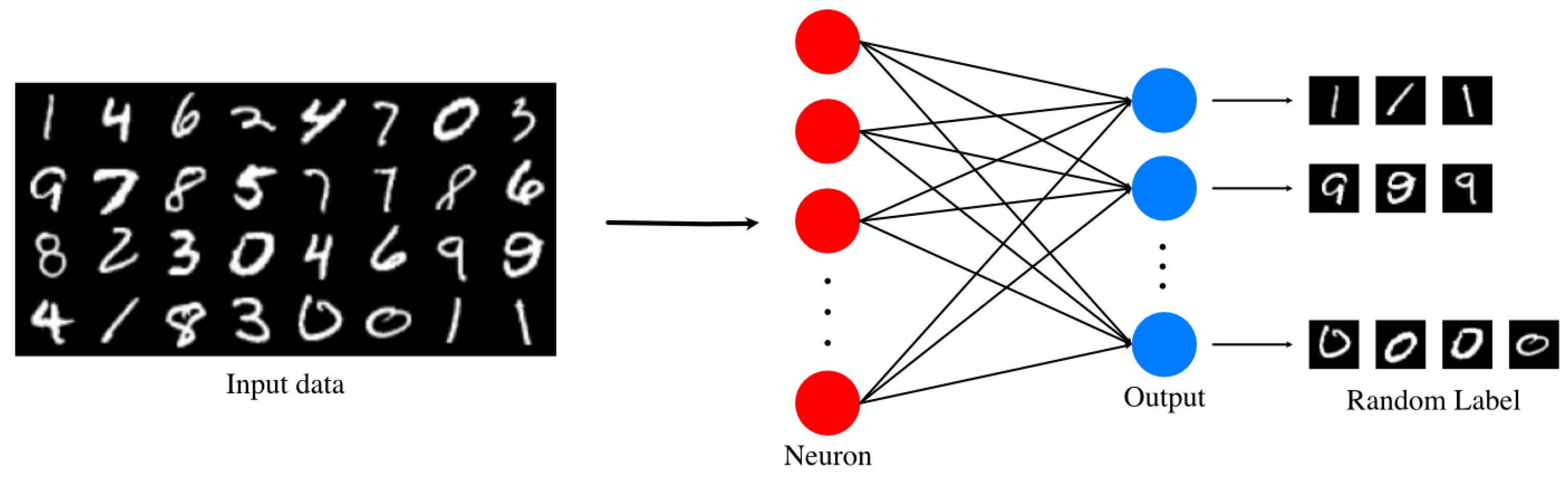
2.1. Unsupervised SNN

SNN can be divided into two types: supervised [17] and unsupervised [16,18] according to the learning method. While the supervised SNN learns with a designated label on each neuron, the unsupervised SNN, as shown in Figure 1, studies the input data by itself without a selected tag on each neuron. The unsupervised SNNs are receiving great attention from both academia and industry due to the characteristic of their learning mechanism being closer to synaptic learning in our brains [19,20,21]. Therefore, this paper also focuses on research on the unsupervised SNN.

Then, recent research on unsupervised SNN can be largely divided into two directions: accuracy improvement and biological model development. Regarding the accuracy improvement study, the training result of the network with two layers using rate coding has shown about 82.9% and 95.0% on average based on 100 and 1600 neurons, respectively, and with subset data using temporal coding have been reported 81.9% cite [18]. Recently, as a learning result by exploiting SVM (Support Vector Machine) and STDP (spike timing dependent plasticity), the accuracy has achieved 98.4% in the network with multiple convolution layers, pooling layer [22].

Many studies have been conducted on the development of neuron models themselves to enhance the the biological meaningfulness of SNN, such as Izhikevich [11], Hodgkin–Huxley [12] and Morris–Lecar [13] models. While the Izhikevich model is made by mathematical analysis of the variation between $N{a}^{+}$ (sodium) channel and $K^{+}$ (potassium) channel, the Hodgkin–Huxley model and Morris–Lecar model is respectively created by modeling the direct variation between $N{a}^{+}$ channel and $K^{+}$ channel and between $C{a}^{2+}$ (calcium) channel and $K^{+}$ channel, both of which are similar to organisms’ adaptation. These three models altogether include the method modulating the frequency of neurons’ reaction, called spike-frequency adaptation, to be evenly fired for stimuli from outside, so the neuron’s activating mechanism is alike modeled on natural organisms’ mechanisms.

Depending on the spike-frequency adaptation method, the Izhikevich, Hodgkin–Huxley, and Morris–Lecar models can be distinguished whether they have biological meaning or just plausibility. First, the Morris–Lecar and Hodgkin–Huxley models create the spike-frequency adaptation by changing the neuron’s potential inclination due to the change of the value of each channel when transmitting data through each channel. It was found in experiments using mice that this modeling is similar to the human neuron communication method [23]. More in detail, the condition in [23] is that a thalamocortical neuron is injected with a $C{a}^{2+}$ buffer solution, and the other neuron is without the buffer solution. Then, both are stimulated by constant electrical intensity stimuli, and each neuron’s potential change is measured to find out how to affect the $C{a}^{2+}$ channel organism’s adaptation. The result showed that the neuron with the $C{a}^{2+}$ buffer solution has adaptation, but the other does not. Plus, the adaptation has shown the inclination change, but not that of the threshold voltage. Therefore, the adaptation is induced by changing the neuron’s potential inclination since the Morris–Lecar and Hodgkin–Huxley models that use the change of the neuron’s potential inclination to implement the adaptation. In other words, since adaptation using the change in potential inclination of the Hodgkin–Huxley, and Morris–Lecar models is the same as that of real organisms, these models can be said to be biologically meaningful.

On the other hand, the Izhikevich model implements the spike-frequency adaptation by changing the threshold voltage ($V_{th}$) of neurons or directly applying electrical current. More specifically, the Izhikevich model adapts by applying different methods to two types of neurons: excitatory and inhibitory cortical cells. In the excitatory cortical cells, regular spiking that remains the neurons’ fire constantly through the inject dc-current, and in the inhibitory cortical cells, using the adaptation, called low-threshold spiking, that increases the parameter of the derived function of membrane recovery variable so that reducing $V_{th}$. Thus, considering the real organism’s adaptation, the Izhikevich model can be regarded as plausible, but not meaningful.

2.2. Neuron Model and Learning Method

Conduct based leaky-integrated and fire model is the most widely-used neuron model equation in SNN [16], which expresses the potential V of neurons over time t by the following formula using the parameters summarized in

Table 1. Parameter descriptions in the neuron model.

Parameter	Description
$E_{rest}$	resting membrane potential
$E_{exc}$	excitatory postsynaptic potential
$E_{inh}$	inhibitory postsynaptic potential
${\tau }_{g_e}$	excitatory conductance time constant
${\tau }_{g_i}$	inhibitory conductance time constant
$g_e$	the conductance associated with the excitatory neuron
$g_i$	the conductance associated with the inhibitory neuron

:

$$\begin{array}{c}\hfill \tau \frac{\mathrm{d}V}{\mathrm{d}t}=(E_{rest}-V)+g_e(E_{exc}-V)+g_i(E_{inh}-V),\end{array}$$

(1)

where $\tau$ is time constant of inherent neuron both excitatory and inhibitory; $E_{rest}$, $E_{exc}$, and $E_{inh}$ are potentials of resting membrane, excitatory postsynaptic, and inhibitory postsynaptic, respectively. In this equation, the spike from outside affects the neuron’s conductance $g_e$, resulting in the neuron’s potential change. After accumulating potential, if the potential is more than $V_{th}$, the neuron fires and creates a spike. In the output neuron, the inference of input data is produced through the created spikes.

The expression of synapse changed by the spike is as follows:

$$\begin{array}{c}\hfill {\tau }_{g_e}\frac{\mathrm{d}{g}_e}{\mathrm{d}t}=-g_e,\end{array}$$

(2)

$$\begin{array}{c}\hfill {\tau }_{g_i}\frac{\mathrm{d}{g}_i}{\mathrm{d}t}=-g_i,\end{array}$$

(3)

where, ${\tau }_{g_e}$, ${\tau }_{g_i}$, $g_e$, and $g_i$ are described in Table 1. More precisely, (2), (3) are the equations of the excitatory synapse and inhibitory synapse, respectively, and the spikes in the neurons through both synapses change each conductance. As a result, the value of $g_e$ and $g_i$ of (1) is changed, so the potential of the neuron is altered.

For learning for SNN, STDP is the most broadly used method [24,25,26,27,28]. In STDP, $W\left(t\right)$ is the value of intensifying or abating synapse weight, which can be formulated as follows [27,28]:

$$\begin{array}{cc}W\left(t\right)=\hfill & \left\{\begin{array}{c}{A}_{+}\left(e^{-\frac{t}{{\tau }_{+}}}\right):\mathrm{if}t\ge 0\hfill \\ -A_{-}\left(e^{\frac{t}{{\tau }_{-}}}\right):\mathrm{otherwise},\hfill \end{array}\right.\end{array}$$

(4)

where A is a parameter connecting intensity between pre-neuron and post-neuron, and $\tau$ is the time difference between pre-spike and post-spike. In this equation, the sign of $\tau$ is determined by the sequence of pre-spike and post-spike, and if the sign is minus as post-spike arrives before pre-spike, there is no correlation of firing spike in the relationship. Hence, the intensity of the connection of each neuron is undermined. Conversely, if the sign is plus, there is a correlation, so the intensity of each neuron’s connection becomes stronger. This is because pre-spike is fired after arriving pre-spike. In addition, if the firing time between pre-spike and post-spike is the same, the weight keeps the value because there is no correlation and the priority of the times is challenging to observe. Finally, there may be a case where only the post-spike is observed and the pre-spike is not observed. In this case, the spike has to be never spiked in any case and non-correlation, so the original weight value is updated by subtracting the designated value.

Next, when defining $\Delta w$ as the weight variation between ith pre-neurons connected to the jth post-neuron, we can express $\Delta w$ as follows:

$$\begin{array}{c}\hfill \Delta w=W(t_j-t_i).\end{array}$$

(5)

The sign of $\Delta w$ is determined by (5), and the outcome affects $learning w$, which is the value that limits the weight values from 0 to 1. More precisely, $learning w$ is described by:

$$\begin{array}{c}\hfill learning w=\left\{\begin{array}{c}{w}_{max}-w_{t-1}\mathrm{if}\Delta w\ge 0\\ w_{t-1}-w_{min}\mathrm{otherwise},\end{array}\right.\end{array}$$

(6)

where $w_{max}$ and $w_{min}$ are the maximum and minimum weight, respectively.

Consequently, according to the above formula, the weight value indicating the strength of the connectivity between jth post-neuron and ith pre-neuron, $w_t^{j,i}$, is updated with the following equation:

$$\begin{array}{c}\hfill w_t^{j,i}=w_{t-1}^{j,i}+\eta \Delta w{\left(learningw\right)}^{\mu },\end{array}$$

(7)

where $\eta$ is the learning rate, and $\mu$ is the value that represents the dependent value of the previous weight. When the resulting $w_t^{j,i}$ is positive, the higher the previous value is, the lower the weight increases; on the other hand, the lower the previous value is, the higher the weight increases. Conversely, when the resulting $w_t^{j,i}$ is negative, the lower the previous value is, the higher the weight increases; on the other hand, the higher the previous value is, the lower the weight increases. In other words, this characteristic plays a role as if any input data map the neuron, the connection of the synapses connected with such a neuron can rapidly increase; on the other hand, non-mapped that of other synapses can be fast reduced.

This STDP method effectively demonstrates the display of the intensity of connections between neurons by having the strength of connections, making it the most useful method for learning SNN. However, the STDP method still has its drawbacks in that, as the weight value increases and approaches 1, the increasing size of the weight value decreases, and on the contrary, as the weight approaches 0, the decreasing size of the weight value decreases and does not approach 0. As a result, when the connection strength needs to be increased, the connection strength may not be increased quickly, or when the connection strength needs to be decreased, the connection strength may not be significantly increased at a certain point. That is, the weight, which is a value of the connection strength, may be weak 0 or 1, respectively.

2.3. Spike Frequency Adaptation

Unlike supervised SNN, unsupervised SNN randomly selects neurons that will learn input data, and the weights of the selected neurons are updated according to the STDP rule. Of course, the updated weight is larger than the unupdated weights, so only the updated neurons react to the numerous input data that will follow, resulting in only these neurons being learned. Thus, the learned neurons may be malfunctioning, and the unupdated neurons remain in their initial state.

The spike frequency adaptation is a solution to tackle the aforementioned problem. The existing SNN have the spike-frequency adaptation by adjusting $V_{th}$ depending on the spikes fired by output neurons [16,18,29]. For example, in the representative frequency adaption method [16], when an input spike ignites an excitatory neuron in the network, the fired neuron increases $V_{th}$ by $\theta$, which is 0.05 mV. At the same time, other neurons that do not fire exponentially reduce $V_{th}$. Accordingly, since $V_{th}$ increases, the fired neurons become less likely to fire. In contrast, unfired neurons have a lower $V_{th}$, making them more likely to be fired by input data than before. As such, the frequency adaptation plays a role in inducing all neurons to learn evenly.

Although the frequency adaptation of this $V_{th}$ variation-based method works functionally well in SNN, this method is different from the biological adaptation mechanism. In fact, the biological adaptation has the characteristic that the sense of stimulation gradually becomes dull (e.g., if the same pressure is continuously applied to a specific area of the skin, the degree of pain gradually decreases), which cannot be reflected at all in the $V_{th}$ variation-based method. In this respect, the existing method clearly lacks biological meaning.

3. SNN with Sensory Adaptation: The Proposed Method

SNN is inherently advantageous to low power consumption rather than deep neural network through event-driven computation [30,31]. By developing direct biological meaningfulness in low power, the SNN leads neuromorphic computing to process, adapt, behave, and learn new information in real-time biologically [6]. Considering that the close relationship between biological meaningfulness and low-power operation is the potential that SNNs ultimately have, we pay attention to refining the existing spike-frequency adaptation that shows high feasibility and accuracy but is far deviant from biological meaningfulness [18,32]. More precisely, biological adaptation has the characteristic of gradually responding to stimuli, but existing methods do not reflect this. Therefore, we aim to develop a more biologically meaningful spike frequency adaptation, thereby ultimately realizing low-power SNNs.

We first note the sensory adaptation that occurs in the human nervous system. Sensory adaptation reduces the sensitivity of the neuron’s receptor to the stimulus itself. For example, if we suddenly enter a bright place after being in the dark, we will soon adjust to the brightness, or when we enter the bathroom, we will frown at the bad smell, but soon become insensitive. Focusing on the human sensory adaptation mechanism, we define a new variable called $neuron$ $sensitivity$ in the neuron model and develop a new spike-frequency adaptation method, the sensory adaptation, in a way that regulates the change in slope of the neuron’s potential when stimulated by this numerical change. To provide a clearer explanation, the features of the proposed sensory adaptation are as follows:

• Sensitivity in the sensory adaptation is a completely different concept from $V_{th}$ discussed in Section 2, where $V_{th}$ represents the potential threshold of the neuron, and the sensitivity refers to the sensitivity of the receptor that the neuron receives the stimulus.
• $V_{th}$ in the proposed SNN with sensory adaptation does not change in any case.

We will then continue to provide a detailed description of the network architecture, neuron model, and methodology that we propose and develop for sensory adaptation through subsections.

3.1. Neuron Model and Network Architecture

In order to develop and validate the sensory adaptation, the neuron model and network architecture of the SNN must be firmly defined. To do that, we have first developed an SNN architecture to be compact and highly efficient. As described in Figure 2, we have adopted a representative SNN architecture in [16] for our baseline architecture. This architecture consists of the input layer and output layer: the input layer comprises 28 × 28 neurons, which is the MNIST pixel size, and the output layer is made up of the excitatory layer and inhibitory layer. In this network architecture, the excitatory and inhibitory layers have the same number of neurons, excitatory and inhibitory neurons, respectively. The connection from the excitatory layer to the inhibitory layer is one-to-one, so individual neurons are connected to each neuron in the same location, such as the connection of the first excitatory neuron and first inhibitory neuron, and the second excitatory neuron and second inhibitory neuron in order. However, the connection from the inhibitory layer to the excitatory layer is all-to-all except for the neuron in the same location, like the first excitatory neuron makes a connection from the 2nd to 99th inhibitory if the total neurons are 100 in each layer.

In the connection from the excitatory layer to the inhibitory layer, the spike of the excitatory neuron stimulates the inhibitory neuron to impede other excitatory neurons’ firing in the excitatory layer. The incited inhibitory neuron stimulates excitatory neurons except for the neuron giving the spike, which causes other excitatory neurons’ inhibitory synapse to hamper their firing, which is called $lateral$ $inhibition$.

The membrane potential of each excitatory and inhibitory neuron can be expressed in order by the following expressions:

$$\begin{array}{c}\hfill {\tau }_e\frac{\mathrm{d}V}{\mathrm{d}t}=(-(V-V_E^{rest})-\frac{g_e}{g_l}(V-V_E)-\frac{g_i}{g_l}(V-V_I)),\end{array}$$

(8)

$$\begin{array}{c}\hfill {\tau }_i\frac{\mathrm{d}V}{\mathrm{d}t}=(-(V-V_I^{rest})-\frac{g_e}{g_l}(V-V_E)),\end{array}$$

(9)

where, (8) is for the excitatory neuron, and (9) is for the inhibitory neuron equation; $V_E^{rest}$ and $V_I^{rest}$ are the resting membrane potential of the excitatory neuron and inhibitory neuron, respectively; $V_E$ and $V_I$ are the membrane potential of the individually excitatory and inhibitory synapses, respectively; and $g_l$ is the own conductance of the neuron.

In addition, ${\tau }_e$ and ${\tau }_i$ in (8) and (9) are the time constant of the excitatory neuron and inhibitory neuron, respectively, whereby the inhibitory neuron biologically has a more extended time constant than the excitatory neuron, so ${\tau }_e<{\tau }_i$. However, both types of neurons have the same value of $V_{th}$ and have the same properties: fire if the membrane potential is greater than $V_{th}$. After firing, they have a different membrane potential $V_E^{reset}$ and $V_I^{reset}$, respectively. Then, if they have reset membrane potential, they cannot change their potential in the period because they cannot accept any spike from outside, which is called $refractory$ $period$. After this period, their potential returns to $V_E^{rest}$ and $V_I^{rest}$, respectively. Finally, detailed values of each parameter we set in the SNN are provided in

Table 2. Parameters in the proposed methodology.

Param.	Value	Param.	Value
$V_E^{rest}$	0.065 V	$V_I$	0.25 V
$V_I^{rest}$	0.06 V	${\tau }_e$	100 ms
$V_E^{reset}$	0.08 V	${\tau }_i$	10 ms
$V_I^{reset}$	0.075 V	${\tau }_{g_e}$	1 ms
$V_{th}$	0.055 V	${\tau }_{g_i}$	2 ms
$V_E$	0V	$g_l$	1 nS

.

$V_I$ suppresses the fire of neurons with relatively low reactivity to input data, allowing only those with relatively high reactivity to that data to fire. In other words, $V_I$ is the parameter that has the greatest influence on the number of neurons learning input data, and by adjusting it, we can reduce unnecessary power consumption by reducing the total number of spikes from the network during test or training. Therefore, we have conducted an experiment to find the optimal $V_I$, which can minimize the number of neurons learning that data when one data is entered in the target network.

To this end, we first fixed at $V_I=0.1$ V, such as previous work [16], and then conducted an experiment, observing that the learning of the winner-take-all (WTA) rule was applied to more than two number of neurons, i.e., input data of the same shape is learned by multiple neurons. To increase training efficiency and reduce power consumption, we then increased $V_I$ to 0.2 V and 0.25 V, which shows that in 0.2 V, the most firing neurons are still more than two, but in 0.25 V, the number is one. In other words, in 0.25 V, only one neuron can fire, so the number of spikes is reduced, and each neuron can have its own data. Therefore, neurons can react more effectively, as they respond to matched data with neuron’s own data if they are stimulated by input spikes. As a consequence, we have set $V_I$ to $0.25$ V, as reported in Table 2.

In addition, the membrane potential of the excitatory synapses, biologically, should be set so as not to suppress neuronal excitability. Therefore, we have set the value of $V_E$ to 0 V. In this way, it is prevented from suppressing the neuron’s excitation and from firing excitedly even in the absence of a spike that stimulates the neuron. Meanwhile, we propose a design by removing the inhibitory synapse from inhibitory neurons, unlike excitatory neurons. This is because an additional inhibitory layer is not required to suppress the inhibitory neurons in the network architecture. As a result of removing the computational part of the inhibitory potential of the inhibitory neuron (cf. no $V_I$ term in (9)) and performing the simulation, we have confirmed that the computational speed of SNN becomes faster while the accuracy remains unchanged compared to the previous work in [16].

3.2. Sensory Adaptation

To begin with, based on (2), the behavioral models of the excitatory and inhibitory synapses can be expressed as follows in order, respectively:

$$\begin{array}{c}\hfill {\tau }_{g_e}\frac{\mathrm{d}{g}_e^t}{\mathrm{d}t}=-g_e^{t-1},\end{array}$$

(10)

$$\begin{array}{c}\hfill {\tau }_{g_i}\frac{\mathrm{d}{g}_i^t}{\mathrm{d}t}=-g_i^{t-1},\end{array}$$

(11)

where, $g_e^t$ and $g_i^t$ are the values of $g_e$ and $g_i$ according to time step.

Next, we have made (10) and (11) into a combined form through Euler’s method, and then added a sensitivity variable for excitatory synapse $g_{Sens}^t$. On the other hand, such a sensitivity variable has not been added to inhibitory synapse, because the inhibitory layer on the network architecture has a structure that fires a value according to the spike output from the excitatory layer connected 1:1, and the inhibitory synapse has the characteristic that it must depend on the excitatory neuron. Finally, the derived models of the excitatory and inhibitory synapses are expressed as follows:

$$\begin{array}{c}\hfill g_e^t=g_e^{t-1}(1-\frac{\Delta t}{{\tau }_{g_e}})+\sum s_l^t{w}_l{g}_{Sens}^t,\end{array}$$

(12)

$$\begin{array}{c}\hfill g_i^t=g_i^{t-1}(1-\frac{\Delta t}{{\tau }_{g_i}})+\sum s_k^t{w}_k,\end{array}$$

(13)

where $s_l^t$ and $s_k^t$ are the spikes from each ith and kth synapses, and $\Delta t$ is the unit time from which spikes come. We have set $\Delta t$ to 1 ms in the simulation.

As the adaptation occurs in the fired neurons, our neural network detects the spikes from the neurons for every $\Delta t$ and generates the adaptation to the fired neurons. $g_{Sens}^t$ of the fired neurons is modulated by the following equation:

$$\begin{array}{c}\hfill g_{Sens}^t=g_{Sens}^{t-1}\times x_{adaptation},\end{array}$$

(14)

where $x_{adaptation}$ is a variable that adjusts $g_{Sens}^t$. Meanwhile, $g_{Sens}^t$ of the neurons except for the fired neurons is recovered through the following equation:

$$\begin{array}{c}\hfill {\tau }_{g_{Sens}}\frac{\mathrm{d}{g}_{Sens}^t}{\mathrm{d}t}=g_{Sens}^{t-1},\end{array}$$

(15)

where ${\tau }_{g_{Sens}}$ is a time constant of $g_{Sens}^t$.

Intensive simulations were performed to analyze the effect of the values of $x_{adaptation}$ and ${\tau }_{g_{Sens}}$ on the results. First, if ${\tau }_{g_{Sens}}$ becomes too large relative to the $x_{adaptation}$ value, the sensitivity of the neuron recovered by ${\tau }_{g_{Sens}}$ becomes smaller than the sensitivity of the neuron reduced by the $x_{adaptation}$ value. Therefore, in this case, the sensitivity of neurons responding to input data is too low, so training and testing take too long, and in serious cases, the sensitivity of neurons converges to zero and causes errors. Next, in the opposite case when ${\tau }_{g_{Sens}}$ becomes too small relative to the $x_{adaptation}$ value, the sensitivity of the neuron recovered by ${\tau }_{g_{Sens}}$ becomes greater than the sensitivity of the neuron reduced by the $x_{adaptation}$. In this case, training itself proceeds properly without errors, but the sensitivity of the neurons is too great to learn the details of data properly, resulting in low accuracy. In the worst case, neurons that cannot fire at all among the neurons in the neural network may result in data and the corresponding label not being mapped to the weight of the neuron. Through these experiments and analyses, we have been able to establish the most appropriate $x_{adaptation}$ and ${\tau }_{g_{Sens}}$ values that harmonized the reduction recovery of sensitivity, resulting in the average of $g_{Sens}^t$ values held by all neurons in the neural network converging to constant numbers during training.

In the end, to verify the effectiveness of the proposed sensory adaptation, we have, respectively, applied the proposed sensory adaptation and the conventional spike-frequency adaptation based on the existing $V_{th}$ variation into the SNN architecture introduced in Section 3.1. As a result, we have confirmed that the accuracy of the simulation to which sensory adaptation is applied is almost the same as that of the simulation to which the conventional method is applied (even the former is slightly higher than the latter), and the total number of spikes fired in the neural network is reduced by about 45% compared to the conventional one. From these results, we have been able to prove that the proposed neuron with sensory adaptation contributes to significantly improving the energy efficiency of SNN by having more biological meaningfulness. Detailed reports and analysis of experimental results are provided in Section 5.

4. Development of the SNN Simulator

To validate the functionality and evaluate the effectiveness of the proposed SNN with the sensor adaptation, we have developed a dedicated SNN simulator using MNIST. The input data of the simulator consists of 60,000 training data and 10,000 test data, both of which are numbers of 0∼9 consisting of 28 × 28 pixels. The input or output data are transformed into a Poisson spike-train through the Poisson process if the network begins to be stimulated, and then transformed spikes stimulate the neurons in the excitatory layer for 350 ms to induce firing. For the transformation, we have divided the input data into eight and change the outcome into the rate by multiplying $interval$, which shows how much to be sensitive about the input spikes. The initial intervalvalue is 2. Then, to transform the value into spikes, if the rate is lower than the uniform random function value, the rate cannot be transformed into a spike, but if not, it can. As in the conventional method [16], if all neurons in the excitatory layer cannot make five spikes for 350 ms, we have designed the simulator to increase the interval one and then repeat the entire process.

The neuron model has been implemented in the form of (8) and (9) by linearizing through Euler’s method, and the synaptic model has also been implemented in the form of (11). Each layer consists of 100 excitatory and inhibitory neurons, respectively. Meanwhile, we have developed a simulator to selectively operate the conventional or our proposed spike-frequency adaptation method. For the existing method, we have developed $V_{th}$ variation-based adaptation in the same way as [16] by increasing $V_{th}$ to a constant number and decreasing exponentially. For the sensory adaptation, linearization of (12) and (13), and (15) for recovery has been implemented. In addition, the refractory periods of excitatory neurons and inhibitory neurons were set to 5 ms and 2 ms, respectively, identical to [16].

The overall progress of the network on the simulator is as follows. First, when a specific excitatory neuron is fired by input data and learned, the weight of the neuron increases the correlation between the number to be learned and specific data of the same number according to the STDP learning rule, and between neurons that output similar data to the corresponding data. Conversely, if the causal relationship between pre-spike and post-spike is unclear in the excitatory neuron (e.g., after a post-spike comes out, a pre-spike comes out, or a post-spike comes out even though there is no pre-spike), the corresponding weight value gradually decreases, weakening the correlation. Weights updated through STDP are subjected to weight normalization, and parts observed with too few neuron connections in the weight (including unobserved parts) are weakened through weight normalization. Afterwards, the learned neurons in the excitatory layer have the learned number mapped to their label. In more detail, we cut the total training data by 10,000 each and after learning, the most learned label was designated as the label of the corresponding neuron. Learning is performed through a total of 180,000 iterations, and when learning is completed, the completed label is designated as the final label of the neurons.

Finally, Figure 3 shows an example of the training result of the simulator. Specifically, Figure 3a,b are the results of 180,000 number of iterations (NOI) applying the $V_{th}$ variation-based adaptation and the sensory adaptation, respectively. As seen in the figures, all the neurons successfully have their own label and data after the training.

We have uploaded the developed simulator online, which is available on https://github.com/ignim/SNN_Sensory (accessed on 1 November 2022).

5. Results

5.1. Experimental Works

We have performed SNN simulations applying the spike-frequency adaptation based on the $V_{th}$ variation and the proposed sensory adaptation using the developed simulator. What we have focused on in the experiment was to figure out how many spikes are generated when sensory adaptation is adopted while showing a similar level of accuracy to the conventional method. For this, we have performed training and testing phases of 180,000 and 10,000 iterations based on [16], respectively.

Figure 4 shows the training results. Figure 4a,b, which are the results of applying the conventional $V_{th}$ variation-based adaptation, describe the changes in $V_{th}$ and the number of spikes caused by the change in $V_{th}$ of neurons according to the NOI, respectively. Figure 4c,d, which are the results from the sensory adaptation, show the change of the number of spikes due to the change of $g_{Sens}^t$ and the change of $g_{Sens}^t$ of the synapse according to the NOI, respectively.

More specifically, in Figure 4a, $V_{th}$ continues to increase until 60,000th iterations before learning all training data, and then $V_{th}$ increases/decreases to similar numbers from 70,000th after learning all training data. This is because the $V_{th}$ variation-based adaptation adds a user-set threshold potential to $V_{th}$ of neurons selected for adaptation for an increase in $V_{th}$ and reduces $V_{th}$ of the remaining unselected neurons exponentially. That is, due to the continuous addition of the user-set value to $V_{th}$ of neurons, learning does not proceed properly from the 70,000th, which requires fine tuning, so that the increase and decrease are repeated as shown in the figure. The aftermath of this appears as a result of the total number of spikes fired fluctuating from the 70,000th as shown in Figure 4b.

On the other hand, in the case of sensory adaptation, the sensitivity ($g_{Sens}^t$) of the neurons selected for the sensory adaptation is multiplied by a certain number to decrease, and that of the remaining unselected neurons increases exponentially. Therefore, both the degree of decrease and increase in sensitivity show a tendency to decrease as learning progresses, and eventually, the sensitivity value converges to a certain value. Figure 4c clearly shows this tendency, after 60,000 iterations, the decreasing inclination of $g_{Sens}^t$ is reduced following the iterations, and finally, the inclination is converged to zero. The aftermath of this phenomenon is also reflected in the change in the total number of spikes of the neural network shown in Figure 4d. As the sensitivity value converges to a certain value, it can be seen from the figure that the total number of spikes fired is also converging to a certain value.

Next, we analyzed the number of spikes fired according to the iteration change. First, through Figure 4b, we can see that the number of spikes fired increases dramatically from the 10,000th iteration. This is because the decrease in the number of firing spikes in the neural network, which can be expected through an increase in $V_{th}$, becomes slower as the adaptation is almost completed at around the 10,000th iteration, whereas, since the training of the neural network has not yet been completed, the weights grow in value through learning until the 60,000th iteration required to learn all the training data afterwards, which can be interpreted as affecting the increase in the number of spikes fired. On the other hand, looking at Figure 4d), we can observe that the number of the firing spikes in the neural network steadily increase until about the 50,000th iteration for the sensory adaptation, and then decrease from about the 60,000th iteration. From this, we can estimate that by the 60,000th iteration, growing weights through learning has a decisive effect on the number of spikes fired change, and then the number of spikes decreases by replacing the role.

Analyzing the number of spikes according to the NOI, we faced the question of whether the point at which the learning of the sensory adaptation is completed was slower than the conventional $V_{th}$ variation-based adaptation. To answer this question, we first look at Figure 5a,c, which show the 10,000th learning result to which the conventional and proposed adaptations are applied, respectively. It can be confirmed that there are neurons that have not yet been trained, and it can be seen that there are more untrained neurons in the result of the proposed method. This might make us doubt that the question was true, but fortunately, if taking a look at the results when all the training data have been trained (at 60,000th) shown in Figure 5b,d, we can confirm that it is not. That is, as can be seen from Figure 5d, in the simulation to which the proposed adaptation is applied, when learning is completed, all neurons are correctly mapped as shown in Figure 5b. In other words, we confirm that the sensory adaptation also shows the same result as the learning rate of the conventional adaptation. In addition, comparing Figure 3a vs. Figure 5b, and Figure 3b vs. Figure 5d, respectively, shows that the numbers in the results at the 180,000th iteration have a darker color overall compared to the corresponding numbers in the results at the 60,000th iteration. This may be because, in the learning after 60,000th, weight tuning is performed for detailed responses of neurons to input data rather than learning for data/label mapping.

Finally, when measuring the number of spikes fired that occurred during a total of 180,000 iterations in the case of the conventional adaptation and sensory adaptation, it can be confirmed that in the former case, an average of 437,447 spikes occurred, whereas in the latter case, an average of 294,584 spikes occurred. That is, by applying the sensory adaptation, the number of spikes in the SNN is reduced to 32.66% compared to the conventional one. Moreover, when the learning is longer than 180,000 iterations, the degree of reduction becomes larger, which means that the low-power superiority of the proposed method can be further increased.

In addition, as reported in

Table 3. Simulation results of the accuracy and number of fired spikes for the conventional and proposed methods.

	Accuracy	Number of Fired Spikes
Conventional method	80.52%	446,722
Proposed method	83.56%	242,904

, when testing is performed using the training results, the accuracy of the SNN with the conventional adaptive method is 80.52%, and the total number of spikes fired under conditions with an average interval of 2.008 is 446,722. In comparison, the average accuracy of SNN using the sensory adaptation was 83.56%, the average interval was 2.0088, and the total number of spikes was 242,904. In other words, the proposed method proves to have low power excellence also in testing, in that the number of spikes fired becomes reduced to 45.63% compared to the previous one while maintaining performance.

5.2. Analysis

We have conducted an analysis to find out more about how the change in frequency adaptation affects the decrease in number of spikes. To this end, $V_{th}$ and $g_{Sens}^t$ of the network have been experimented with changing in the test environment, while all the remaining control variables, such as weights and neural labels, have been set to fixed values. $V_{th}$ and $g_{Sens}^t$ were changed by 0.001 V and 0.05, respectively, which reduces the number of spikes to the same level in SNN using conventional or sensory adaptations.

The results of the $V_{th}$ change in Figure 6a show that the decreasing slope of the number of spikes from −0.055 V to −0.054 V (cf. the gray line in the figure) is steeper than that caused by other changes, and the rate of variation tends to decrease as $V_{th}$ increases. Contrary to this, in the case of the sensory adaptation shown in Figure 6b, it can be seen that if $g_{Sens}^t$ is reduced, the inclination of the decline of the number of spikes increases. To analyze the results of this experiment, we have created a simple network of one input neuron and one excitation neuron. This network does not have inhibitory neurons because it is intended only to observe the movement of the potential of neuron.

The voltage charging model of the RC circuit allows us to simulate the potential movement of neurons, so the resulting changes in the potential of neurons due to stimuli outside the network can be shown in Figure 7. The potential change over time can be expressed as follows:

$$\begin{array}{c}\hfill V=V_0\left(1-e^{-\frac{t}{\tau }}\right)+V_{offset},\end{array}$$

(16)

where $\tau$, $V_0$, and $V_{offset}$ are the time constant of the neuron, the voltage made by input spikes, and the voltage offsetting the potential of the neuron, respectively. Then, (16) is converted to the following expression to calculate the time it takes V to reach $V_{th}$ from $V_E^{rest}$. For reference, V is expressed as $V_{th}^{dynm}$ to emphasize that it is a dynamically changing variable.

$$\begin{array}{c}\hfill t=-\tau ln\left(1-\frac{V_{th}^{dynm}-V_{offset}}{V_0}\right).\end{array}$$

(17)

If the potential of a neuron is greater than or equal to $V_{th}^{dynam}$, the potential drops to $V_E^{rest}$ and then follows (16). That is, if a constant intensity spike stimulates the neuron, the neuron will be fired at regular intervals. Therefore, it is possible to infer how many spikes are generated in the network, and the total number is described as follows.

$$\begin{array}{c}\hfill S_{prod}=-\frac{S_{total}}{\tau ln\left(1-\frac{V_{th}^{dynm}-V_{offset}}{V_0}\right)},\end{array}$$

(18)

where $S_{prod}$ and $S_{total}$ are the number of fired spikes and input spikes, respectively. Moreover, in a spike train in which spikes are injected per unit time, $S_{total}$ can be regarded as simulation time. Therefore, we can derive (17) from (18), and based on this expression, we can proceed with an analysis of why power reduction occurs when $V_{th}$ or $g_{Sens}^t$ changes.

We differentiate (18) to find out the variation of $S_{prod}$ per $V_{th}^{dynam}$, which is a decrease in the slope of the number of the fired spikes, to find out why increasing $V_{th}$ reduces the total firing spikes. The derived expression is as follows:

$$\begin{array}{c}\hfill \begin{array}{c}\hfill \frac{d{S}_{prod}}{d{V}_{th}^{dynm}}={\displaystyle \frac{S_{\mathrm{total}}/{ln}^2\left(1-\frac{V_{th}^{dynm}-V_{\mathrm{offset}}}{V_0}\right)}{\tau ·\left(V_{th}^{dynm}-V_{\mathrm{offset}}-V_0\right)}}\end{array}\end{array}$$

(19)

$V_{th}^{dynm}$ ranges from $V_E^{rest}$ to steady state voltage, and the inclination is always minus in this range. In addition, in this range, if $V_{th}^{dynm}$ increases, the inclination is increased, which means that the absolute value of the inclination becomes reduced. Hence, as the decline of the inclination of total firing spikes equals the absolute value, the total firing spikes in the SNN with $V_{th}$ variation-based adaptation must be consistently decreased if $V_{th}$ is increased.

Meanwhile, in Figure 6a, it can be observed that the total number of fired spikes remains from about 171,000 to 189,000 at the moment of reaching a certain level of $V_{th}$. This is due to an increase in the interval of the neural network. In other words, as $V_{th}$ increases, the total spike decreases and the number of spikes is smaller than the minimum spike for inference, so the neural network proceeds with the inference by increasing the interval. This soon leads to a decrease in the number of total fired spikes. Therefore, the number of output spikes fired according to the change of the interval becomes a steady-state fluctuation.

Next, in the case of the proposed sensory adaptation, as shown in Figure 6b, the decrease in the number of spikes generated by the neural network increases as $g_{Sens}^t$ is decreased. To analyze this, we can express (16) as follows.

$$\begin{array}{c}\hfill V=\alpha V_0\left(1-e^{-\frac{t}{\beta \tau }}\right)+V_{offset},\end{array}$$

(20)

where $\alpha$ and $\beta$ are values dependent on $g_{Sens}^t$ and are proportional to $g_{Sens}^t$. In the RC circuit model, the change in $g_{Sens}^t$ affects the spike supplied to the neuron and the conductance of the neuron, which affects $V_0$ and $\tau$ in (16), so we introduce $\alpha$ and $\beta$. We then express the time required for neurons to reach $V_{th}$ from $V_E^{rest}$ to $V_{th}$ in order to determine the reason for the increasing size of the number of spikes created by neural networks with sensory adaptation:

$$\begin{array}{c}\hfill t=-\beta \tau ln\left(1-\frac{V_{th}-V_{offset}}{\alpha V_0}\right).\end{array}$$

(21)

Similar to the one that induced (18), we can derive $S_{prod}$ from (21) and it is described as follows:

$$\begin{array}{c}\hfill S_{prod}=-\frac{S_{total}}{\beta \tau ln\left(1-\frac{V_{th}^{dynm}-V_{offset}}{\alpha V_0}\right)}.\end{array}$$

(22)

In this equation, $\alpha$ and $\beta$ are proportional to the change in $g_{Sens}^t$, so we replace them with $l·g_{Sens}^t$ and $k·g_{Sens}^t$, respectively. Subsequently, the result of obtaining the slope of $S_{prod}$ is as follows:

$$\begin{array}{c}\hfill \frac{d{S}_{prod}}{d{V}_{th}^{dynm}}={\displaystyle \frac{S_{\mathrm{total}}}{k\tau ln\left(1-\frac{V_{\mathrm{th}}-V_{\mathrm{offset}}}{V_{0}l{g}_{Sens}^t}\right)g_{Sens}^{2t}}}+\\ \hfill {\displaystyle \frac{\left(V_{\mathrm{th}}-V_{\mathrm{offset}}\right)S_{\mathrm{total}}}{V_{0}kl\tau {ln}^2\left(1-\frac{V_{\mathrm{th}}-V_{\mathrm{offset}}}{V_{0}l{g}_{Sens}^t}\right)\left(1-\frac{V_{\mathrm{th}}-V_{\mathrm{offset}}}{V_{0}l{g}_{Sens}^t}\right)g_{Sens}^{3t}}}\end{array}$$

(23)

In this equation, $\frac{d{S}_{prod}}{d{V}_{th}^{dynm}}$ can have a positive value when the neuron’s steady state voltage is higher than $V_{th}$, so $\frac{d{S}_{prod}}{d{V}_{th}^{dynm}}$ is declined when $g_{Sens}^t$ increases. From this, we are able to infer that when $g_{Sens}^t$ decreases, $\frac{d{S}_{prod}}{d{V}_{th}^{dynm}}$ increases, so the inclination value of the total spikes also increases, as shown in Figure 6b. In other words, according to $g_{Sens}^t$ goes from 1 to 0, the inclination value increases, as described with the blue line in Figure 6b, which is steeper than the gray line that shows the inclination when $g_{Sens}^t$ is changed from 1 to 0.95. Therefore, the number of spikes fired is reduced depending on the decline of $g_{Sens}^t$.

In addition, we can identify this phenomenon in the change of the neuron’s steady state voltage due to $g_{Sens}^t$ change. In Figure 8, the neuron’s steady state voltage is more changed depending on the decline of $g_{Sens}^t$, similar to the blue line in Figure 6b. Since the steady state voltage depends on $V_0$ change, the inclination of the change of the steady state voltage affects $\tau$ in (20), which is the inclination. Therefore, the steady state voltage can also explain why the total spikes reduction happens.

Finally, in Figure 6b, the SNN with $Sensory Adaptation$ generates the terminal total spikes from about 100,000 to 120,000, where $g_{Sens}^t$ is lower than 0.2. This phenomenon happens because of the same reason for $V_{th}$ variation. We can find out that $Sensory Adaptation$ is more significant to reduce power consumption compared with two total spikes made by $Sensory Adaptation$ and $V_{th}$ variation. Therefore, we can also re-identify the cause of the increase in the reduction in the amount of fired spikes, which was derived with (21)–(23) via Figure 8.

6. Discussion

We propose the sensory adaptation that is closer to the biological adaptation mechanism and develop a more biologically meaningful SNN that applies it. We develop a software simulator to verify the effectiveness of the corresponding SNN, which proves that the developed SNN can maintain the same accuracy while generating fewer firing spikes. This means that when SNN is implemented as a semiconductor chip, the chip operates with low power. More specifically, in a chip operating at a nominal voltage, the dynamic power is the dominant of the total power consumption [33,34,35]. In an SNN chip, the dynamic power is directly proportional to the number of fired spikes. Therefore, as the number of fired spikes decreases, the SNN chip operates with less power consumption.

However, this paper does not place the scope on implementing the developed SNN in hardware. Therefore, we do not consider the design and implementation overhead that results when the proposed technique is implemented in real hardware. For future work, we plan to design a SNN with proposed method as analog circuits and fabricate it into a chip, and in this process, we will be able to achieve the development of optimization design techniques and demonstrate the effectiveness of the proposed SNN with the silicon-proven SNN chip.

7. Conclusions

Motivated by the expectation that there may be a strong relationship between SNN biological significance and low-power driving, this paper aimed to focus on spike-frequency adaptation, which deviates significantly from existing biological meaningfulness, and to develop a new spike-frequency adaptation with more biological characteristics. To this end, we proposed a sensory adaptation method focusing on the mechanism by which human sensory organs reduce sensitivity to stimuli, and studied the network architecture and neuron model to apply it. Subsequently, we developed a dedicated SNN simulator that can selectively apply the existing $V_{th}$-based adaptation and the proposed sensory adaptation, and conducted functional verification and effectiveness evaluation of the proposed method using this simulator. We intensively performed simulation, revealing that the proposed more biologically meaningful adaptation can achieve similar performance as before, firing only a significantly reduced number of spikes to 32.66% and 45.63% in training and testing, respectively. From the viewpoint of implementing SNN as a semiconductor chip, based on the fact that the largest power consumption of an SNN chip is determined by how many spikes are fired, the results of the lower number of fired spikes in the developed SNN confirms that the proposed method can achieve a low-power SNN chip. Furthermore, we conducted an in-depth analysis of how this benefit is obtained, and ultimately contributed to SNN research by providing an example and analysis results that incorporate biological meanings into SNN and may be closely related to the low-power driving characteristics of SNN.

References

1. Davies, M. Advancing Neuromorphic Computing from promise to Competitive technology. In Proceedings of the Neuro-Inspired Computational Elements Workshop (NICE), Albany, NY, USA, 26–28 March 2019. [Google Scholar]
2. Merolla, P.A.; Arthur, J.V.; Alvarez-Icaza, R.; Cassidy, A.S.; Sawada, J.; Akopyan, F.; Jackson, B.L.; Imam, N.; Guo, C.; Nakamura, Y.; et al. A million spiking-neuron integrated circuit with a scalable communication network and interface. Science 2014, 345, 668–673. [Google Scholar] [CrossRef] [PubMed]
3. Benjamin, B.V.; Gao, P.; McQuinn, E.; Choudhary, S.; Chandrasekaran, A.R.; Bussat, J.M.; Alvarez-Icaza, R.; Arthur, J.V.; Merolla, P.A.; Boahen, K. Neurogrid: A Mixed-Analog-Digital Multichip System for Large-Scale Neural Simulations. Proc. IEEE 2014, 102, 699–716. [Google Scholar] [CrossRef]
4. Akopyan, F.; Sawada, J.; Cassidy, A.; Alvarez-Icaza, R.; Arthur, J.; Merolla, P.; Imam, N.; Nakamura, Y.; Datta, P.; Nam, G.J.; et al. TrueNorth: Design and Tool Flow of a 65 mW 1 Million Neuron Programmable Neurosynaptic Chip. IEEE Trans. Comput.-Aided Des. Integr. Circuits Syst. 2015, 34, 1537–1557. [Google Scholar] [CrossRef]
5. Davies, M.; Srinivasa, N.; Lin, T.H.; Chinya, G.; Cao, Y.; Choday, S.H.; Dimou, G.; Joshi, P.; Imam, N.; Jain, S.; et al. Loihi: A Neuromorphic Manycore Processor with On-Chip Learning. IEEE Micro 2018, 38, 82–99. [Google Scholar] [CrossRef]
6. Davies, M.; Wild, A.; Orchard, G.; Sandamirskaya, Y.; Guerra, G.A.F.; Joshi, P.; Plank, P.; Risbud, S.R. Advancing Neuromorphic Computing with Loihi: A Survey of Results and Outlook. Proc. IEEE 2021, 109, 911–934. [Google Scholar] [CrossRef]
7. Khodaverdian, Z.; Sadr, H.; Edalatpanah, S.A. A Shallow Deep Neural Network for Selection of Migration Candidate Virtual Machines to Reduce Energy Consumption. In Proceedings of the 2021 7th International Conference on Web Research (ICWR), Tehran, Iran, 19–20 May 2021; pp. 191–196. [Google Scholar]
8. Khodaverdian, Z.; Sadr, H.; Edalatpanah, S.A.; Solimandarabi, M.N. Combination of Convolutional Neural Network and Gated Recurrent Unit for Energy Aware Resource Allocation. arXiv 2021, arXiv:2106.12178. [Google Scholar]
9. Shukla, R.; Khalilian, B.; Partouvi, S. Academic progress monitoring through neural network. Big Data Comput. Visions 2021, 1, 1–6. [Google Scholar]
10. Peykani, P.; Eshghi, F.; Jandaghian, A.; Farrokhi-Asl, H.; Tondnevis, F. Estimating cash in bank branches by time series and neural network approaches. Big Data Comput. Visions 2021, 1, 170–178. [Google Scholar]
11. Izhikevich, E. Simple model of spiking neurons. IEEE Trans. Neural Netw. 2003, 14, 1569–1572. [Google Scholar] [CrossRef] [Green Version]
12. Hodgkin, A.L.; Huxley, A.F. A quantitative description of membrane current and its application to conduction and excitation in nerve. J. Physiol. 1952, 117, 500. [Google Scholar] [CrossRef]
13. Morris, C.; Lecar, H. Voltage oscillations in the barnacle giant muscle fiber. Biophys. J. 1981, 35, 193–213. [Google Scholar] [CrossRef] [Green Version]
14. Izhikevich, E. Which model to use for cortical spiking neurons? IEEE Trans. Neural Netw. 2004, 15, 1063–1070. [Google Scholar] [CrossRef]
15. Peron, S.P.; Gabbiani, F. Role of spike-frequency adaptation in shaping neuronal response to dynamic stimuli. Biological cybernetics. Biol. Cybern. 2009, 100, 505–520. [Google Scholar] [CrossRef]
16. Diehl, P.; Cook, M. Unsupervised learning of digit recognition using spike-timing-dependent plasticity. Front. Comput. Neurosci. 2015, 9, 99. [Google Scholar] [CrossRef] [Green Version]
17. Kulkarni, S.R.; Alexiades, J.M.; Rajendran, B. Learning and real-time classification of hand-written digits with spiking neural networks. In Proceedings of the 2017 24th IEEE International Conference on Electronics, Circuits and Systems (ICECS), Tehran, Iran, 19–20 May 2017. [Google Scholar]
18. Daqi Liu, S.Y. Fast unsupervised learning for visual pattern recognition using spike timing dependent plasticity. Neurocomputing 2017, 249, 212–224. [Google Scholar]
19. Kang, T.; Oh, K.I.; Lee, J.J.; Kim, S.E.; Kim, S.E.; Lee, W.; Oh, W. Spiking Neural Networks-Inspired Signal Detection Based on Measured Body Channel Response. IEEE Trans. Instrum. Meas. 2022, 71, 1–16. [Google Scholar] [CrossRef]
20. Kang, T.; Hwang, J.H.; Kim, H.; Kim, S.E.; Oh, K.I.; Lee, J.J.; Park, H.I.; Kim, S.E.; Oh, W.; Lee, W. Measurement and Evaluation of Electric Signal Transmission Through Human Body by Channel Modeling, System Design, and Implementation. IEEE Trans. Instrum. Meas. 2021, 70, 1–14. [Google Scholar] [CrossRef]
21. Barbier, T.; Teulière, C.; Triesch, J. Spike timing-based unsupervised learning of orientation, disparity, and motion representations in a spiking neural network. In Proceedings of the 2021 IEEE/CVF Conference on Computer Vision and Pattern Recognition Workshops (CVPRW), Nashville, TN, USA, 19–25 June 2021; pp. 1377–1386. [Google Scholar]
22. Kheradpisheh, S.R.; Ganjtabesh, M.; Thorpe, S.J.; Masquelier, T. STDP-based spiking deep convolutional neural networks for object recognition. Neural Netw. 2018, 99, 56–67. [Google Scholar] [CrossRef] [Green Version]
23. Ha, G.E.; Lee, J.; Kwak, H.; Song, K.; Kwon, J.; Jung, S.Y.; Hong, J.; Chang, G.E.; Hwang, E.M.; Shin, H.S.; et al. The Ca2+-activated chloride channel anoctamin-2 mediates spike-frequency adaptation and regulates sensory transmission in thalamocortical neurons. Nat. Commun. 2016, 7, 13791. [Google Scholar] [CrossRef]
24. Morrison, A.; Aertsen, A.; Diesmann, M. Spike-Timing-Dependent Plasticity in Balanced Random Networks. Neural Comput. 2007, 19, 1437–1467. [Google Scholar] [CrossRef]
25. Nessler, B.; Pfeiffer, M.; Buesing, L.; Maass, W. Bayesian Computation Emerges in Generic Cortical Microcircuits through Spike-Timing-Dependent Plasticity. PLoS Comput. Biol. 2013, 9, e1003037. [Google Scholar] [CrossRef] [PubMed] [Green Version]
26. Pfister, J.P.; Gerstner, W. Triplets of Spikes in a Model of Spike Timing-Dependent Plasticity. J. Neurosci. 2006, 26, 9673–9682. [Google Scholar] [CrossRef] [PubMed] [Green Version]
27. Song, S.; Miller, K.D.; Abbott, L.F. Competitive Hebbian learning through spike-timing-dependent synaptic plasticity. Nat. Neurosci. 2000, 3, 919–926. [Google Scholar] [CrossRef] [PubMed]
28. Bi, G.q.; Poo, M.m. Synaptic Modifications in Cultured Hippocampal Neurons: Dependence on Spike Timing, Synaptic Strength, and Postsynaptic Cell Type. J. Neurosci. 1998, 18, 10464–10472. [Google Scholar] [CrossRef] [Green Version]
29. Doborjeh, M.; Doborjeh, Z.; Merkin, A.; Bahrami, H.; Sumich, A.; Krishnamurthi, R.; Medvedev, O.N.; Crook-Rumsey, M.; Morgan, C.; Kirk, I.; et al. Personalised predictive modelling with brain-inspired spiking neural networks of longitudinal MRI neuroimaging data and the case study of dementia. Neural Netw. 2021, 144, 522–539. [Google Scholar] [CrossRef]
30. Guo, S.; Wang, L.; Wang, S.; Deng, Y.; Yang, Z.; Li, S.; Xie, Z.; Dou, Q. A Systolic SNN Inference Accelerator and Its Co-Optimized Software Framework. In Proceedings of the 2019 on Great Lakes Symposium on VLSI, Tysons Corner, VA, USA, 9–11 May 2019; pp. 63–68. [Google Scholar]
31. Li, S.; Zhang, Z.; Mao, R.; Xiao, J.; Chang, L.; Zhou, J. A Fast and Energy-Efficient SNN Processor With Adaptive Clock/Event-Driven Computation Scheme and Online Learning. IEEE Trans. Circuits Syst. Regul. Pap. 2021, 68, 1543–1552. [Google Scholar] [CrossRef]
32. Querlioz, D.; Bichler, O.; Dollfus, P.; Gamrat, C. Immunity to Device Variations in a Spiking Neural Network with Memristive Nanodevices. IEEE Trans. Nanotechnol. 2013, 12, 288–295. [Google Scholar] [CrossRef] [Green Version]
33. Lee, W.; Kang, T.; Lee, J.J.; Han, K.; Kim, J.; Pedram, M. TEI-ULP: Exploiting Body Biasing to Improve the TEI-Aware Ultralow Power Methods. IEEE Trans. Comput.-Aided Des. Integr. Circuits Syst. 2019, 38, 1758–1770. [Google Scholar] [CrossRef]
34. Han, K.; Lee, S.; Lee, J.J.; Lee, W.; Pedram, M. TIP: A Temperature Effect Inversion-Aware Ultra-Low Power System-on-Chip Platform. In Proceedings of the 2019 IEEE/ACM International Symposium on Low Power Electronics and Design (ISLPED), Lausanne, Switzerland, 29–31 July 2019; pp. 1–6. [Google Scholar]
35. Han, K.; Lee, S.; Oh, K.I.; Bae, Y.; Jang, H.; Lee, J.J.; Lee, W.; Pedram, M. Developing TEI-Aware Ultralow-Power SoC Platforms for IoT End Nodes. IEEE Internet Things J. 2021, 8, 4642–4656. [Google Scholar] [CrossRef]
Figure 1. Unsupervised SNN: the input data gone into the network are processed by output neurons and printed out through the synapses connected with the output neurons. The 10 labels in the input data map each of the 10 neurons to a different number. When mapped, the output labels are random rather than sequential in numerical order.
Mathematics 10 04191 g001
Figure 2. The SNN architecture of this paper consists of an input layer, an excitatory layer, and an inhibitory layer, and contains 784, 100, and 100 neurons, respectively.
Mathematics 10 04191 g002
Figure 3. Weight results of neurons according to 180,000 number of iterations (NOI) when (a) the conventional V t h variation-based adaptation and (b) the sensory adaptation is applied.
Mathematics 10 04191 g003
Figure 4. Trainingsimulation results: When using the V t h variation-based adaptation, (a) the change in V t h and (b) total number of spikes fired according to NOI changes, and when using the proposed sensory adaptation, (c) the change in g S e n s t and (d) total number of spikes fired according to NOI changes.
Mathematics 10 04191 g004
Figure 5. Weight results of neurons according to (a) 10,000 NOI and (b) 180,000 NOI when the conventional V t h variation-based adaptation is applied, and (c) 10,000 NOI and (d) 180,000 NOI when the sensory adaptation is applied.
Mathematics 10 04191 g005
Figure 6. Graph showing the change in the total number of fired neurons according to the change of (a) V t h and (b) g S e n s t .
Mathematics 10 04191 g006
Figure 7. The potential graph of the neuron when the neuron with input and output is stimulated for 350 ms.
Mathematics 10 04191 g007
Figure 8. The change in steady-state voltage with the change in g S e n s t . The gray line indicates that g S e n s t represents the slope from 1 to 0.95.
Mathematics 10 04191 g008